Attentional multi-level representation encoding based on convolutional and variance autoencoders for lncRNA–disease association prediction

Sheng, Nan; Cui, Hui; Zhang, Tiangang; Xuan, Ping

doi:10.1093/bib/bbaa067

Abstract

As the abnormalities of long non-coding RNAs (lncRNAs) are closely related to various human diseases, identifying disease-related lncRNAs is important for understanding the pathogenesis of complex diseases. Most of current data-driven methods for disease-related lncRNA candidate prediction are based on diseases and lncRNAs. Those methods, however, fail to consider the deeply embedded node attributes of lncRNA–disease pairs, which contain multiple relations and representations across lncRNAs, diseases and miRNAs. Moreover, the low-dimensional feature distribution at the pairwise level has not been taken into account. We propose a prediction model, VADLP, to extract, encode and adaptively integrate multi-level representations. Firstly, a triple-layer heterogeneous graph is constructed with weighted inter-layer and intra-layer edges to integrate the similarities and correlations among lncRNAs, diseases and miRNAs. We then define three representations including node attributes, pairwise topology and feature distribution. Node attributes are derived from the graph by an embedding strategy to represent the lncRNA–disease associations, which are inferred via their common lncRNAs, diseases and miRNAs. Pairwise topology is formulated by random walk algorithm and encoded by a convolutional autoencoder to represent the hidden topological structural relations between a pair of lncRNA and disease. The new feature distribution is modeled by a variance autoencoder to reveal the underlying lncRNA–disease relationship. Finally, an attentional representation-level integration module is constructed to adaptively fuse the three representations for lncRNA–disease association prediction. The proposed model is tested over a public dataset with a comprehensive list of evaluations. Our model outperforms six state-of-the-art lncRNA–disease prediction models with statistical significance. The ablation study showed the important contributions of three representations. In particular, the improved recall rates under different top |$k$| values demonstrate that our model is powerful in discovering true disease-related lncRNAs in the top-ranked candidates. Case studies of three cancers further proved the capacity of our model to discover potential disease-related lncRNAs.

lncRNA–disease association prediction, deep learning, convolutional and variance autoencoders, representation-level attention

Introduction

Long non-coding RNAs (lncRNAs), with a length of more than 200 nucleotides, are one type of non-coding RNAs [1–4]. Accumulating evidences demonstrated that the abnormalities of lncRNAs are linked with progression of various diseases [5–9]. Thus, identifying disease-related lncRNAs will contribute to the exploration of the pathogenesis of the diseases and the promotion of disease diagnosis and treatment.

Recently, computerized prediction models have been developed for miRNA–disease association prediction [10, 11], drug–target interaction prediction [12, 13], synergistic drug combination prediction [14, 15] and lncRNA–disease association prediction [16, 17]. The computerized screening can reduce the costs and time consuming in biomedical experiments. Machine learning models have attracted increasing attention in disease-related lncRNA screening because of the capacity in estimating lncRNA–disease associations using diverse data, which provides potential disease-related lncRNA candidates for biologists to discover true lncRNAs with further experiments [18]. According to the diversity of data sources involved in computing, there are two categories of models for disease–lncRNA association prediction. One category focuses on modeling the similarities of lncRNAs and diseases, while the other one utilizes multiple sources of data apart from lncRNAs and diseases such as miRNAs, proteins and genes. The 1st computational model in the field of lncRNA–disease association prediction was proposed by Chen et al. [19]. The model, known as LRLSLDA, is based on Laplacian regularized least squares, which predicts the candidate lncRNA–disease associations from the known lncRNA–disease associations and lncRNA expression profiles. This semi-supervised approach inspires subsequent research on computerized lncRNA–disease association prediction. Ping et al. [20] proposed a flow propagation algorithm based classifier to integrate two kinds of lncRNA similarities and two disease similarities that were calculated by a lncRNA–disease heterogeneous network. Non-negative matrix factorization [21–23] and graph models [24–27] have also been explored to integrate the lncRNA–disease similarities and associations. Sun et al. [28] constructed a graph of lncRNA similarities and exploited random walk with restart (RWR) algorithm for disease-related lncRNA prediction. A further work by Gu et al. [29] proposed a heterogeneous graph to integrate the similarities of diseases, lncRNAs and lncRNA–disease associations to predict the possibility of lncRNA–disease associations. The aforementioned models, however, failed to consider diverse sources of information, which are related with lncRNAs and diseases such as miRNAs and proteins.

The 2nd category of methods considers other sources of data apart from lncRNAs and diseases. For instance, disease-related lncRNAs were predicted based on flow propagation algorithm over a lncRNA–protein–disease network [30]. Lan et al. [31] proposed a support vector machine (SVM) based classifier to integrate two kinds of lncRNA similarities and five disease similarities. Ding et al. [32] estimated the lncRNA–disease association scores by constructing a lncRNA–disease-gene network and resource allocation mechanism. Similarly, a network of lncRNAs, diseases and miRNAs was constructed by Yu et al. [33], where a Naive Bayes classification model was used for association estimation. Fan et al. [34] integrated the expressions of lncRNAs, miRNAs and proteins and used RWR model to derive potential lncRNA–disease associations. There are also a couple of methods based on matrix factorization for multi-source data integration [35–37]. Wang et al. [38] developed a data fusion method based on selective matrix factorization, which collaboratively decomposes multiple interrelated data matrices into low-rank representation matrices for each object type and optimizes their weights. Even though multiple sources of data were considered in the models mentioned above, these models were not able to discover the underlying and complex relationship of lncRNAs and diseases because of the shallow level integration of cross-modality similarities.

With the development of deep learning algorithms, recent models further improved the prediction performance by extracting deep and complementary features. A dual convolutional neural network (CNN) was proposed by Xuan et al. [39] to predict disease-related lncRNAs. A more recent graph CNN model was exploited by [40]. These two deep models, however, failed to integrate the node attributes and feature distributions of lncRNA–disease at pairwise level. Even though deep models demonstrated improved performance in lncRNA–disease association prediction, CNN-based models cannot effectively integrate and learn correlations from non-grid structural heterogenous data such as miRNA, lncRNA and disease. To learn from heterogenous data, recent research in social network and recommender systems shows that attribute information and topological information contribute to the improvement performance in neural networks [41–44].

In this work, we propose a prediction model, VADLP, to learn, encode and adaptively integrate multi-level representations including pairwise topology, node attributes and feature distributions from multi-sourced data. The contributions of our model are included:

A multi-layer heterogenous graph is constructed to benefit the extraction of a newly introduced representation of node attributes for lncRNA–disease association modeling. The graph is composed of weighted inter- and intra-layer edges to embed similarities and correlations across multiple sources of data including lncRNAs, diseases and miRNAs. Pairwise node attributes are derived from the heterogeneous graph by a proposed embedding mechanism based on biological premises that if a pair of lncRNA and disease has associations or similarities with common lncRNAs, miRNAs or diseases, there is high probability that the lncRNA and disease are associated.
We took the initiative to introduce feature distribution, which is modeled by variance autoencoder (VAE), to reveal the underlying relationship and facilitate lncRNA–disease association prediction. The feature distribution is a high-level representation learnt and encoded from original node attributes.
We propose a pairwise topology encoding module to learn the hidden topological structural relations between a pair of lncRNA and disease. The pairwise topology representation is firstly formulated by applying random walk algorithm over the multi-layer heterogeneous graph and then encoded by a convolutional autoencoder (CAE).
An attentional representation-level integration and optimization module is proposed to enable the adaptive fusion of pairwise topology, node attributes and feature distribution. The contributions of three representations and capacity of the proposed model for disease-related lncRNA prediction are demonstrated by a comprehensive list of evaluations including ablation study, comparison with recent published models and case studies of three diseases.

Materials and Methods

The framework of the proposed VADLP model for lncRNA–disease association prediction is given in Figure 1. We firstly construct a triple-layer heterogeneous graph with weighted inter-layer and intra-layer edges to associate the similarities and correlations among lncRNAs, miRNAs and diseases. The representations of node attributes, pairwise topology and feature distribution are learned, respectively. Finally, these three representations are adaptively fused by attentional integration mechanism for further estimating the association possibility of a pair of lncRNA and disease.

Dataset

A public dataset for lncRNA–disease association prediction is obtained from [35], which contains 240 lncRNAs, 495 miRNAs and 405 diseases. The available information includes 2687 lncRNA–disease associations extracted from LncRNADisease database [45], 1002 pairs of lncRNA–miRNA interactions obtained from starBasev2.0 [47] and 13 559 pairs of miRNA–disease association obtained from HMDD [48]. Disease names are obtained from the US National Library of Medicine (MeSH, http://www.ncbi.nlm.nih.gov/mesh).

Triple-layer heterogeneous graph

We construct a weighted graph |$\textrm{G}{ \textrm{=}} \left ( {V,E,\textbf{W}} \right )$| with lncRNA-, miRNA- and disease-based layers, where nodes |$ V = \big \{{V^{lncRNA}}\cup{V^{miRNA}}\cup{V^{disease}}\big \}$| are composed of sets of lncRNA |${V^{lncRNA}}$|⁠, miRNA |${V^{miRNA}}$| and disease |${V^{disease}}$| and an edge |${e_{ij}} \in E$| links a pair of nodes |$v_{i},v_{j} \in V$| undirectedly with weight |$w_{ij}\in \textbf{W}$|⁠. According to the types of nodes connected by the edge, there are intra-layer and inter-layer edges. As shown in Figure 2, we define weight matrix |${\bf W}\, =\, ({\bf A,S})$| with inter-association matrix A and intra-similarity matrix S for inter- and intra-layer edges, respectively. Inter-association matrices denote whether the relations between different types of nodes are available or not. Intra-similarity matrices represent the similarities between the same type of nodes.

The inter-association weight matrix A is defined as

$$\begin{equation} \textbf{A}=\left\{{\begin{array}{l} \textbf{A}^{lncRNA-disease}\in{{\mathbb{R}^{N_{V^{lncRNA}}\times{N_{V^{disease}}}}}},\\ \qquad\textrm{if}\;{v_i} \in{V^{lncRNA}},{v_j} \in{V^{disease}};\\ \textbf{A}^{miRNA-disease}\in{{\mathbb{R}^{N_{V^{miRNA}}\times{N_{V^{disease}}}}}},\\ \qquad\textrm{if}\;{v_i} \in{V^{miRNA}},{v_j} \in{V^{disease}};\\ \textbf{A}^{lncRNA-miRNA}\in{{\mathbb{R}^{N_{V^{lncRNA}}\times{N_{V^{miRNA}}}}}};\\ \qquad\textrm{if}\;{v_i} \in{V^{lncRNA}},{v_j} \in{V^{miRNA}},\\ \end{array}}\right. \end{equation}$$

(1)

where |$A_{ij} \in{ \textbf{A}^{lncRNA-disease}\big ({{\textbf{A}}^{miRNA-disease}}\big )}= 1$| if a lncRNA (miRNA) node |$v_{i}$| and a disease node |$v_{j}$| is related according to the LncRNADisease database (HMDD) [45, 48], |$A_{ij}=0$| otherwise. |${\textbf{A}}^{lncRNA-miRNA}$| is defined to assist the prediction of lncRNA–disease associations because it has been proved that there are interactions between lncRNAs and miRNAs involved in the disease process [49, 50]. |$A_{ij} \in{\textbf{A}}^{lncRNA-miRNA}=1$| if the interaction between a pair of lncRNA and miRNA nodes has been observed according to starBasev2.0 database, |$A_{ij}=0$| otherwise.

Intra-similarity matrix S for intra-edges is defined as

$$\begin{equation} \textbf{S}=\left\{{\begin{array}{l} \textbf{S}^{disease}=\big({S}_{ij}^{disease}\big)\in{{\mathbb{R}^{N_{V^{disease}}\times{N_{V^{disease}}}}}},\\ \qquad\textrm{if}\;{v_i},{v_j} \in{V^{disease}};\\ \textbf{S}^{lncRNA}=\big({S}^{lncRNA}\big)\in{{\mathbb{R}^{N_{V^{lncRNA}}\times{N_{V^{lncRNA}}}}}},\\ \qquad\textrm{if}\;{v_i},{v_j} \in{V^{lncRNA}};\\ \textbf{S}^{miRNA}=\big({S}^{miRNA}\big)\in{{\mathbb{R}^{N_{V^{miRNA}}\times{N_{V^{miRNA}}}}}},\\ \qquad\textrm{if}\;{v_i},{v_j} \in{V^{miRNA}},\\ \end{array}}\right. \end{equation}$$

(2)

where |${\textbf{S}}^{disease}$| is calculated to reflect the disease semantic similarities and |${\textbf{S}}^{lncRNA}\big ({\textbf{S}}^{miRNA}\big )$| represents the similarities between a pair of lncRNA (miRNA). |$S_{ij}^{disease} \in \left [{0,1}\right ]$| is calculated based on the directed acyclic graph of diseases that was proposed by Wang et al. [51]. Step-by-step calculation of |$S_{ij}^{disease}$| is given in Supplementary File SF1.

|${S_{ij}^{lncRNA}}$| and |$S_{ij}^{miRNA}$| are calculated via related diseases of a pair of lncRNAs or miRNAs by the method proposed by Chen et al. and Wang et al. [51, 52], respectively. Suppose |$i$|-th lncRNA |$v_{i}^{lncRNA}$| is associated with a set of diseases |$\Phi _{i}^{lncRNA} = {\Big \{ {d_{ik}|k=1\ldots N_{\Phi _{i}^{lncRNA}}} \Big \}}$|⁠, lncRNA |$v_{j}^{lncRNA}$| is associated with a set of diseases |$\Phi _{j}^{lncRNA} =\Big \{ {d_{jl}|l=1\ldots N_{\Phi _{j}^{lncRNA}}} \Big \}$|and |$S_{ij}^{lncRNA}$| is obtained by measuring the similarity between |$\Phi _{i}^{lncRNA}$| and |$\Phi _{j}^{lncRNA}$|⁠. Similarly, |$S_{ij}^{miRNA}$| is calculated by the similarity between associated disease sets |$\Phi _{i}^{miRNA}$| and |$\Phi _{j}^{miRNA}$|⁠. Detailed calculations of |${S_{ij}^{lncRNA}}$| and |$S_{ij}^{miRNA}$| are given in Supplementary File SF1. In addition, the calculation results for |${S_{ij}^{lncRNA}}$| and |$S_{ij}^{miRNA}$| are shown in SF2 and SF3, respectively.

Given the graph model, association matrix |$\rm \textbf{A}$| and similarity matrix |$\rm \textbf{S}$|⁠, the heterogenous weight matrix |${\textbf{W}}= \left ({w_{ij}}\right ) \in \mathbb{R}^{N_{V}\times N_{V}}$| where |$N_{V}=N_{V^{lncRNA}}+ N_{V^{disease}}+N_{V^{miRNA}} $| is summarized as below to integrate the intra-layer similarities and inter-layer associations

$$\begin{equation} \textbf{W}\!=\! \begin{bmatrix} \textbf{S}^{lncRNA}& \textbf{A}^{lncRNA-disease}& \textbf{A}^{lncRNA-miRNA}\\{\textbf{A}^{lncRNA-disease}}^{\textrm{T}} & \textbf{S}^{disease} & {\textbf{A}^{miRNA-disease}}^{\textrm{T}}\\{\textbf{A}^{lncRNA-miRNA}}^{\textrm{T}} & \textbf{A}^{miRNA-disease} & \textbf{S}^{miRNA} \end{bmatrix}, \end{equation}$$

(3)

where |$ {\rm \textbf A}^{\textrm{T}}$| denotes the transpose matrix of |$\rm \textbf A$|⁠.

Pairwise topology extraction by random walk

To fully utilize the topological structural relations among lncRNA–disease–miRNA embedded in the graph G, we formulate the pairwise topology by random walk algorithm [53] to assist the lncRNA–disease association prediction.

To learn the pairwise topology between |$m$|-th RNA and |$n$|-th disease, we suppose a random walker starts from a node of |$m$|-th lncRNA |$v_{m}^{lncRNA}\in V^{lncRNA}$| and |$n$|-th disease |$v_{n}^{disease}\in V^{disease}$|⁠. The walker iteratively transmits to its neighboring node via the connecting edge with the probability that is proportional to the edge weight. The higher the weight, the easier the transition.

Given weight matrix |$\rm \textbf{W}$|⁠, the status |$\vec{\pi }_{m}^{lncRNA}\left ({t+1}\right )$| of the walker reaching node |$v_{i}$| at time |$t+1$| by initially starting from |$v_{m}^{lncRNA}$| is formulated by equation (4) as

$$\begin{equation} \vec \pi _m^{lncRNA}\left( {t + 1} \right) = \left( {1 - \beta} \right) \textbf{U} \vec \pi _m^{lncRNA}\left( t \right) + \beta \vec \pi _m^{lncRNA}\left( 0 \right), \end{equation}$$

(4)

where |$\vec{\pi }_{m}^{lncRNA}\left ({t+1}\right )=\left [{{\pi }_{im}^{lncRNA}\left ({t+1}\right )}\right ]_{1\times N_{V}}$|⁠, |${\pi }_{m}^{lncRNA}\left ({t+1}\right )$| is the probability that a random walker reaching node |$v_{i}$| at time |$t+1$| and |$\vec{\pi }_{m}^{lncRNA}\left ({0}\right )$| is the initial one-hot vector where |$\pi _{mm} \left ({0}\right )=1$| and 0 elsewhere. |$\textbf{U}_{N_{V}\times N_{V}}$| is the transpose of row-normalized weight matrix |$\rm \textbf{W}$| and |$u_{ij}\in \textbf{U}$| is the transition probability from node |$v_{i}$| to |$v_{j}$|⁠.

Fig. 1

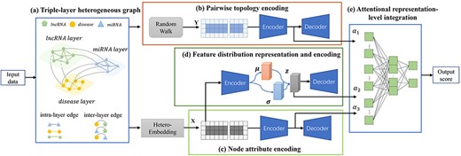
Framework of the proposed VADLP model. Given input data, (A) triple-layer heterogeneous graph is constructed to associate the similarities and correlations across lncRNAs, miRNAs and diseases with inter- and intra-layer weighted edges. Three representations are learned including (B) pairwise topology encoding by random walk and CAE, (C) node attributes by a proposed heterogeneous embedding mechanism and CAE and (D) feature distribution representation and encoding by VAE. The three representations are adaptively fused by (E) attentional representation-level integration for final lncRNA–disease association prediction. Details of each component are given in Fiures 2–4.

Open in new tab Download slide

Fig. 2

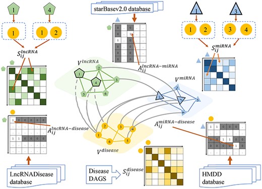
Inter-association and intra-similarity matrices A and S derived from the multi-layer heterogeneous graph of lncRNA, miRNA and disease.

Open in new tab Download slide

The transition process is converged when the following |$L_{1}$| norm is satisfied

$$\begin{equation} \min{\left\| {\vec \pi _m^{lncRNA}\left( {t + 1} \right) - \vec \pi _m^{lncRNA}\left( t \right)} \right\|_1} < 1{0^{ - 6}} \end{equation}$$

(5)

and the steady-state matrix |$\vec{\pi }_{m}^{lncRNA}\left ({\infty }\right )_{1\times N_{V}}$| that the random walker will finally stay at node |$v_{i}\in V$| is obtained. As |$\rm \textbf{W}$| embeds intra-layer similarities and inter-layer associations, |$\vec{\pi }_{m}^{lncRNA}\left ({\infty }\right )$| represents the associations, similarities and interactions among lncRNAs, diseases and miRNAs while enhanced by graph topology. A higher value of |$\pi _{im}^{lncRNA}\in \vec{\pi }_{m}^{lncRNA}\left ({\infty }\right )$| indicates a closer relation between a pair of |$v_i$| and |$v_{m}^{lncRNA}$|⁠.

Fig. 3

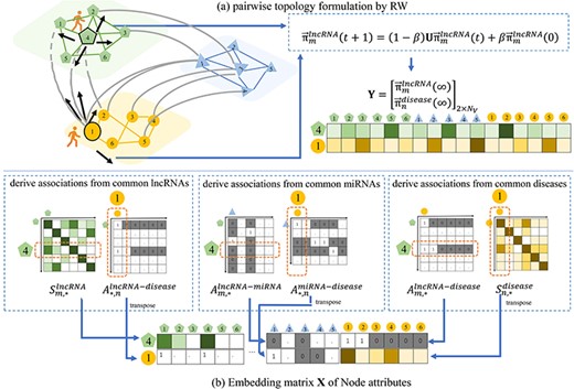
Illustration of extraction process of the proposed pairwise topology and node attributes between a pair of lncRNA and disease. Given 4th lncRNA and 1st disease as an example, (A) the pairwise topology is obtained as the steady-state status of RW over the graph, and (B) the embedding matrix of node attributes are derived from the graph weights via the common lncRNAs, miRNAs and diseases.

Open in new tab Download slide

Similarly, we can obtain the steady-state matrix |$\vec{\pi }_{n}^{disease}\left ({\infty }\right )$| of the random walker starting from |$n$|-th disease node |$v_n^{disease}\in{V^{disease}}$|⁠. The final pairwise topology matrix Y is obtained by embedding |$\vec{\pi }_{m}^{lncRNA}\left ({\infty }\right )$| and |$\vec{\pi }_{n}^{disease}\left ({\infty }\right )$| from top to bottom as shown in Figure 3A as

$$\begin{equation} \textbf{Y} \textrm{=} {\left[{\begin{array}{*{20}{l}} {\vec \pi _m^{lncRNA}\left( \infty \right)}\\{\vec \pi _n^{disease}\left( \infty \right)} \end{array}} \right]_{2 \times{N_V}}}. \end{equation}$$

(6)

Heterogenous node attributes extraction by embedding strategy

We propose an embedding strategy to derive heterogeneous node attribute between a pair of lncRNA and disease from inter-layer associations and intra-layer similarities. The embedding strategy is based on the biological premise that for a pair lncRNA and disease with unknown association, if they have associations or similarities with common lncRNAs, miRNAs or diseases, there are high probabilities that the lncRNA and disease are associated.

Given inter-association matrices |$\textbf{A}^{lncRNA-disease}$|⁠, |$ \textbf{A}^{miRNA-disease}$| and |$\textbf{A}^{lncRNA-miRNA}$| and intra-similarity matrices |$\textbf{S}^{disease}$| and |${\textbf{S}}^{lncRNA}$|⁠, the embedding matrix |$\rm \textbf{X}$| of node attributes between |$m$|-th lncRNA |$v_m^{lncRNA}$| and |$n$|-th disease |$v_n^{disease}$| is obtained by the following procedure as shown in Figure 3B. Firstly, to embed the associations derived from common lncRNAs, the |$m$|-th row of |${\textbf{S}}^{lncRNA}$|⁠, |$S_{m,*}^{lncRNA}$|⁠, is combined with transposed |$n$|-th column of |${\textbf{A}}^{lncRNA-disease}$|⁠, |$A_{*,n}^{{lncRNA-disease}^{\textrm{T}}}$|⁠, as

$$\begin{equation} {X_1} = \left[{S_{m, *} ^{lncRNA};A_{ *,n}^{lncRNA - diseas{e^{\textrm{T}}}}} \right], \end{equation}$$

(7)

where |$S_{m,*}^{lncRNA}$| contains the similarities between |$v_m^{lncRNA}$| and all the lncRNAs and |$A_{*,n}^{lncRNA-disease}$| records the associations between |$v_n^{disease}$| and all the lncRNAs. Secondly, to embed interactions derived via common miRNAs, the |$m$|-th row of |${\textbf{A}}^{lncRNA-miRNA}$| and transposed |$n$|-th column of |${\textbf{A}}^{miRNA-disease}$| are concatenated as

$$\begin{equation} {X_2}\textrm{=} \left[{A_{m, * }^{lncRNA - miRNA};A_{ *,n}^{miRNA - diseas{e^{\textrm{T}}}}} \right], \end{equation}$$

(8)

where |$A_{m,*}^{lncRNA-miRNA}$||$\big ({A_{*,n}^{miRNA-disease}}\big )$| contains the interactions (associations) between |$v_m^{lncRNA}$||$\big ({v_n^{disease}}\big )$| and all the miRNAs. Lastly, to embed the correlations derived through common diseases, the |$m$|-th row of |${\textbf{A}}^{lncRNA-disease}$| and |$n$|-th row of |${\textbf{S}}^{disease}$| are concatenated as

$$\begin{equation} {X_3} = \left[{A_{m, *} ^{lncRNA - disease};S_{n, *} ^{disease}} \right], \end{equation}$$

(9)

where |$A_{m,*}^{lncRNA-disease}$| contains associations between |$v_m^{lncRNA}$| and all the diseases and |$S_{n,*}^{disease}$| records the similarities between |$v_n^{disease}$| and all the diseases. The final embedding matrix |${\textbf{X}}\in \mathbb{R}^{2\times N_V} $| is obtained as

$$\begin{equation} \begin{split} \textbf{X}& \!=\! \begin{bmatrix} X_{1}& X_{2}& X_{3} \end{bmatrix}\\ &\!=\!\begin{bmatrix} {S_{m, *} ^{lncRNA}}&{A_{m, *} ^{lncRNA - miRNA}}&{A_{m, * }^{lncRNA - disease}}\\{A_{ *,n}^{\ln cRNA - diseas{e^{\textrm{T}}}}}&{A_{ *,n}^{miRNA - diseas{e^{\textrm{T}}}}}&{S_{n, *} ^{disease}} \end{bmatrix}. \end{split} \end{equation}$$

(10)

Multi-level knowledge encoding

As the matrices of pairwise topology and node attributes obtained from the graph model are sparse high-dimensional matrices, there may be useless and non-presentative information. To learn deep while discriminative node attributes and topology from the original data distribution, CAE is used for encoding and decoding. To derive implicit representative feature distributions to assist prediction, VAE module is used. The overview of the proposed method is shown in Figure 1.

Pairwise topology encoding by CAE

Given matrix Y, a CAE is constructed to encode pairwise topological representation as shown by Figure 4A.

Fig. 4

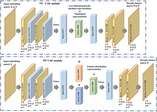
Parameter settings of (A) CAE and (B) VAE. s denotes stride, k denotes kernel and p is the padding.

Open in new tab Download slide

Encoder. The encoder is composed of two hidden layers where each layer consists of a convolutional layer and a max-pooling layer as shown by Figure 4A. To preserve and learn the marginal information of Y, zeros padding is performed to Y. The 1st hidden layer takes zero-padded Y as input and gives an output feature map |$ \textrm{Y}_{encode}^{\left ({1}\right )}$| as

$$\begin{equation} \textrm{Y}_{encode}^{\left( 1 \right)} = max\left( {\sigma \left( {W_{encode}^{\left( 1 \right)} * \textbf{Y} + b_{encode}^{\left( 1 \right)}} \right)} \right). \end{equation}$$

(11)

Zero padding is performed to preserve the marginal information of Y. The feature map |$\textrm{Y}_{encode}^{\left ({k}\right )}$| of the |$k$|-th layer is calculated as

$$\begin{equation} \begin{split} \textrm{Y}_{encode}^{\left( k \right)} \!=\! max\left( {\sigma \left( {W_{encode}^{\left( k \right)} * \textrm{Y}_{encode}^{\left( {k - 1} \right)} + b_{encode}^{\left( k \right)}} \right)} \right),\\ k \!=\! 2, \cdots{L_{AE}}, \end{split} \end{equation}$$

(12)

where |$L_{AE}$| is the total number of encoder layersand |$W_{encode}^{\left ({k}\right )}$| and |$b_{encode}^{\left ({k}\right )}$| are weight matrix and bias vector for the |$k$|-th hidden layer, respectively. ‘|$\ast $|’ is the convolution operator. |$\sigma =\textrm{max}(0,x)$| is the ReLU activation function where max represents the max-pooling layer that is used to down-sample the latent representation after the convolutional layer and captures the most important feature in each feature map.

Decoder. To obtain the most optimized encoded feature map, we project |$\textrm{Y}_{encode}^{\left ({L_{AE}} \right )}$| back to the original space by a decoder so that we can calculate the errors between the decoded matrix and original matrix Y. The decoder is constructed with three hidden layers where each hidden layer includes a transposed convolutional layer. Given |$ \textrm{Y}_{encode}^{\left ({L_{AE}}\right )}$| as the input of the first decoder layer, a feature map |$\textrm{Y}_{decode}^{\left ({1}\right )}$| is obtained as

$$\begin{equation} \textrm{Y}_{decode}^{\left( 1 \right)} = \sigma \left( {W_{decode}^{\left( 1 \right)} \star \textrm{Y}_{encode}^{\left( {{L_{AE}}} \right)} + b_{decode}^{\left( 1 \right)}} \right) \end{equation}$$

(13)

and the feature map of the |$l$|-th hidden decoder layer is

$$\begin{equation} \begin{split} \textrm{Y}_{decode}^{\left( l \right)} = \sigma \left( {W_{decode}^{\left( l \right)} \star \textrm{Y}_{decode}^{\left( {l - 1} \right)} + b_{decode}^{\left( l \right)}} \right),\\ l = 2, \cdots{L_{DE}}, \end{split} \end{equation}$$

(14)

where |$L_{DE}$| is the total number of decoder layersand |$W_{decode}^{\left ({l} \right )}$| and |$b_{decode}^{\left ({l}\right )}$| are the weight matrix and bias vector of the decoder layer, respectively. ‘|$\star $|’ denotes the transpose convolution operator. The reconstructed matrix |$\hat{\textbf{Y}}$| is obtained as the output |$\textrm{Y}_{decode}^{\left ({L_{DE}} \right )}$| of the last decoder layer.

Optimization. Mean-square error is used as the loss function to measure the error between the |$\hat{\textbf{Y}}$| and Y as

$$\begin{equation} los{s_1} = \frac{1}{{{N_{train}}}}{\sum\nolimits_{i = 1}^{{N_{train}}} {\left( {\textrm{Y}_i - {{\hat{\textrm{Y}}}_i}} \right)} ^2}, \end{equation}$$

(15)

where |$\textrm{Y}_i$| is the embedding matrix of the |$i$|-th lncRNA–disease pair in the training set and |$\hat{\textrm{Y}}_i$| is the corresponding reconstructed matrix through the decoding layer. |$N_{train}$| is the number of training samples. The loss function (15) is optimized by Adam algorithm [54]. The CAE is trained by the backpropagation (BP) algorithm [55]. When |$loss_1$| is minimized, the output of the last encoder layer is considered as the deep pairwise topology representation, which is denoted by |$\mathcal{F}_{topology}$|⁠.

Node attribute encoding by CAE

Similarly, a CAE module is constructed for the embedding matrix X to encode node attributes of a pair of lncRNA–disease. The settings for encoder and decoder are the same as that for pairwise topology encoding with details given in Figure 4A. We denote the encoded pairwise node attributes of the |$m$|-th lncRNA and |$n$|-th disease after the training process by |$\mathcal{F}_{attribute}$|⁠.

Feature distribution representation and encoding by VAE

Apart from |$\mathcal{F}_{attribute}$| learnt from the original node attributes, we introduce representative feature distribution, which is derived from node attributes by VAE. Our hypothesis is that the feature distribution would serve as complementary information to further improve the prediction performance.

A VAE module is established as shown in Figure 4B. Matrix X is fed into a variational encoder to learn the feature distribution |$z$| and then |$z$| is sent to decoder to obtain the decoded |$\hat{\textbf{X}} $|⁠. The optimization process aims to minimize the error between |$\hat{\textbf{X}}$| and X.

Variational encoder. The detailed setting of the encoder is illustrated in Figure 4B. The outputs of the 1st and other hidden layers in the encoder are

$$\begin{equation} \textrm{X}_{encode}^{\left( 1 \right)} = max\left( {g\left( {{W^{\left( 1 \right)}} * \textrm{X}{ \textrm{+}} {b^{\left( 1 \right)}}} \right)} \right) \end{equation}$$

(16)

$$\begin{equation} \begin{split} \textrm{X}_{encode}^{\left( k \right)} = max\left( {g\left( {{W^{\left( k \right)}} * {\textrm{X}^{\left( {k - 1} \right)}}{ \textrm{+}}{b^{\left( k \right)}}} \right)} \right),\\ k = 2, \cdots{L_{EN}}, \end{split} \end{equation}$$

(17)

where |$L_{EN}$| is the number of the encoder layers, |$g= \textrm{max}\left ({0,x}\right )$| is the nonlinear activation function ReLU, |$W^{\left ({1}\right )}$| and |$W^{\left ({k}\right )}$| are the weight matrices of the first layer and the |$k$|-th layer, respectively, and |$b^{\left ({1}\right )}$| and |$b^{\left ({k}\right )}$| are the corresponding bias vectors, respectively. ‘|$\ast $|’ denotes the convolution operator. |$max$| is the max-pooling, and the feature map output by the convolutional layer is down-sampled.

To obtain the feature distribution |$z$|⁠, the output of the last encoder layer, |$X_{encode}^{\left ( {{L_{EN}}} \right )}$|⁠, is firstly flattened to be a vector |$X_{encode}^{\left ( {{L_{EN}}} \right )^{\prime}}$|⁠. Then the feature information extracted by the convolutional encoder is represented as |$z=q\left ({z|X}\right )$| by calculating mean and variance

$$\begin{equation} q\left( {z|\textrm{X}} \right) = \prod\nolimits_{i = 1}^n {q\left( {{z_i}| \textrm{X}} \right)} \end{equation}$$

(18)

$$\begin{equation} q\left( {{z_i}|\textrm{X}} \right) = N\left( {{u_i},diag\left( {\sigma _i^2} \right)} \right), \end{equation}$$

(19)

where |$n$| is the dimension of the feature distribution vector |$z$|⁠. |$u$| and |$\sigma $| are the mean and variance vectors of |$X_{encode}^{\left ( {{L_{EN}}} \right )^{\prime}}$|⁠, |${q\left ( {{z_i}|\textrm{X}} \right )}$| represents the parameterized posterior probability, and the feature distribution vector |$z$| is sampled from |$q$|⁠.

Variance decoder. The decoder is a conditional generation model. Let |$p\left ({X|z}\right )$| denote the probability that a given implied variable |$z$| can generate X

$$\begin{equation} p\left( {\textrm{X}|z} \right) = D\left( {\textrm{X}|{f_{decode}}\left( z \right)} \right), \end{equation}$$

(20)

where |$f_{decode}\left ({z}\right )$| is used to parameterize the distribution D. The formula of |$f_{decode}\left ({z}\right )$| is as below:

$$\begin{equation} f_{decode}^{\left( 1 \right)}\left( z \right) = g\left( {{f_{linear}}\left( {W_{decode}^{\left( 1 \right)} z + b_{decode}^{\left( 1 \right)}} \right)} \right) \end{equation}$$

(21)

$$\begin{equation} \begin{split} f_{decode}^{\left( l \right)}\left( z \right) = g\left( {{f_{tranconv}}\left( {W_{decode}^{\left( l \right)} \star f_{decode}^{\left( {l - 1} \right)}\left( z \right) + b_{decode}^{\left( l \right)}} \right)} \right),\\ l = 2, \cdots{L_{DE}}, \end{split} \end{equation}$$

(22)

where |$L_{DE}$| is the number of decoding layers and |$g$| is the activation function ReLU. |$W_{decode}^{\left ({1}\right )}$| and |$b_{decode}^{\left ({1}\right )}$|are the weight matrix and of bias vector of the linear layer, respectively. |$f_{linear}$| is linear operation, and |$f_{tranconv}$| is a transpose convolutional operation. |$f_{decode}^{\left ({1}\right )}{\left ({z}\right )}$| is the feature vector obtained through the linear layer, while |$f_{decode}^{\left ({l}\right )}$| is the feature map obtained through the |$l$|-th layer.

Optimization. We optimize the variational lower bound by the loss defined as

$$\begin{equation} los{s_2} = {E_{q\left( {z|\textrm{X}} \right)}}\left[{\log \left( {p\left( { \textrm{X}|z} \right)} \right)} \right] - KL\left[{q\left( {z|\textrm{X}} \right)||p\left( z \right)} \right], \end{equation}$$

(23)

where |$KL\left [{{q{\left ({\cdot }\right )}}||{p\left ({\cdot }\right )}}\right ]$| is the Kullback–Leibler divergence between |$q\left ({\cdot }\right )$| and |$p\left ({\cdot }\right )$|⁠. |$p\left ({\cdot }\right )$| is a prior distribution, which is a Gaussian distribution |$p\left ({z}\right )={\prod _{i=1}{N\left ({z_i} |0,1\right )}}$| in VADLP. We used the Adam algorithm to optimize |$loss_2$| and BP is performed for training. When the training process is finished, the learnt generative feature distribution is obtained by |$z$| and denoted by |$\mathcal{F}_{feature}$|⁠.

Attentional multi-level representation integration and optimization

To integrate the encoded pairwise topology, node attributes and feature distributions for association prediction, we propose an attentional multi-level representation integration and optimization module. The module can adaptively fuse multi-sourced knowledge by adaptive weights, which are reflected by attentional scores.

Attentional scores. Given the encoded representations |$\mathcal{F} = \{\mathcal{F}_{topology}, \mathcal{F}_{attribute},\mathcal{F}_{feature}\}$|⁠, the informative score |$s_i$| of |$i$|-th representation is calculated as

$$\begin{equation} {s_i} = tanh\left( {{W_{att}}{\mathcal{F} _i} + {b_{att}}} \right), \end{equation}$$

(24)

where |$W_{att}$| is a weight matrix and |$b_{att}$| is a bias vector. The normalized attention score |$\alpha _i$| is

$$\begin{equation} {a_i} = \frac{{exp\left( {s_i^{\textrm{T}}{s_{att}}} \right)}}{{\sum\nolimits_{i \in 3} {exp\left( {s_i^{\textrm{T}}{s_{att}}} \right)}}}, \end{equation}$$

(25)

where |$s_{att}$| is used to capture the context feature vector between three representations. The attention enhanced vector |$\tilde{\mathcal{F}}_i$| is obtained as

$$\begin{equation} {\tilde{\mathcal{F} _i}} = {\alpha _i} \circ \ {\mathcal{F} _i}, \end{equation}$$

(26)

where ‘|$\cdot $|’ denotes the element-wise product operator. A new representation |$\tilde{\mathcal{F}}_{combine}\in{\mathbb{R}^{3N_V\times 1}}$| is obtained by the concatenation of |$\tilde{\mathcal{F}}_i$|⁠.

Optimization and classification. To obtain the association probability |$\phi $| of a pair of lncRNA and disease, a fully connected layer and a softmax layer are applied to |$\tilde{\mathcal{F}}_{combine}$| as shown by Figure 1E. |$\phi $| is defined as

$$\begin{equation} \phi = softmax\left( {{W_{soft}} {{{\tilde{\mathcal{F}} _{combine}}}} + {b_{soft}}} \right), \end{equation}$$

(27)

where |$W_{soft}$| and |$b_{soft}$| are weight matrix and bias vector of softmax layer, respectively. |$\phi =\left [{\phi _1,\phi _2}\right ]$| where |$\phi _1$| is the probability that the lncRNA is associated with the disease, and |$\phi _2$| is the probability that they do not have association relation.

Cross-entropy is used as the loss function for optimizing the classification model, which is defined as

$$\begin{equation} los{s_3} = - \sum\nolimits_{i = 1}^{{N_{train}}} {\left[{{y_{label}}\log \left( \phi_1 \right) + \left( {1 - {y_{label}}} \right)\log \left( {1 - \phi_1} \right)} \right]}, \end{equation}$$

(28)

where |$y_{label}$| represents the actual association case between a lncRNA and a disease. When lncRNA is indeed associated with disease, |$y_{label}=1$|⁠; otherwise, |$y_{label}=0$|⁠. |$loss_3$| is optimized by Adam algorithm.

Experimental results and discussions

Experimental setup and evaluation metrics

Our method is implemented in PyTorch framework on a Nvidia GeForce GTX 2070Ti graphic card with 64G memory. The detailed parameter settings of CAE and VAE are given in Figures 4A and B. The learning rate was set as 0.0001. Dropout strategy |$\left ({P=0.5}\right )$| is performed to reduce the impact of overfitting. The effects of restarting parameter |$\beta $| in random walk algorithm are investigated and given in Supplemental Table ST1. Given |$\beta \in \left [{0.1,0.9} \right ] $|⁠, the best performance was achieved when |$\beta =0.8$|⁠.

Five-fold cross-validation is performed for performance evaluation of all the models in comparison. There are 2687 known lncRNA–disease associations and |$240*405-2687=94513$| unknown associations. All known lncRNA–disease associations are randomly partitioned into five equal-sized sets, where four of them are used for training and the remaining one is used for testing. In each fold, we randomly select lncRNA–disease samples with unobserved associations whose size is equal to that of samples with known associations for training, and the remaining unobserved lncRNA–disease associations are used for testing. The known lncRNA–disease associations are regarded as positive samples, while the unobserved lncRNA–disease associations are regarded as negative samples. The predicted association scores of testing samples are calculated and ranked. The higher the ranking of the positive examples, the better the prediction performance. In particular, in each round of cross-validation, lncRNA–lncRNA similarity is re-calculated by excluding the positive samples, which are to be used for testing. By such, we guarantee that the intra-lncRNA similarities used for graph construction will not contain information of the testing dataset.

Several evaluation measures include receiver operating characteristic (ROC) curve, true positive rate (TPR) and false positive rate (FPR), precision-recall (PR) curve, area under ROC (AUC), area under PR (AUPR) and recall rates under different top |$k$| values. The average AUC and AUPR in the 5-fold cross-validations are used to evaluate the performance of all the models in comparison.

AUC is used for evaluation because it is a well-recognized evaluation index for the comparison of algorithms with probability estimation [56]. ROC is obtained based on the TPR and FPR under various threshold values. For a threshold |$\theta $|⁠, if the predicted lncRNA–disease association score is greater than |$\theta $|⁠, the sample is identified as a positive sample; otherwise, the sample is considered as a negative sample. TPR (FPR) is defined as the proportion of correctly (incorrectly) identified positive (negative) samples among all the positive (negative) samples, which is calculated as

$$\begin{equation} TPR = \frac{{TP}}{{TP + FN}},\quad FPR = \frac{{FP}}{{TN + FP}}, \end{equation}$$

(29)

where |$TP \left ({TN}\right )$| denotes the number of correctly identified positive (negative) samples and |$FN \left ({FP}\right )$| denotes the number of incorrectly identified positive (negative) samples.

Given that the lncRNA–disease candidates with known and unknown associations are imbalanced (1:36), AUPR is more informative than AUC under such circumstances [57]. Thus, AUPR is also used to validate the performance. Precision and recall are defined as

$$\begin{equation} precision = \frac{{TP}}{{TP + FP}},\quad recall = \frac{{TP}}{{TP + FN}}, \end{equation}$$

(30)

where precision represent the percentage of the correctly identified positive samples among all the samples, which are predicted as positive and recall is the same as |$TPR$|⁠. In this work, averaging cross-validation [58] is used to calculate AUC and AUPR values. It means that firstly, we calculate the average AUC or AUPR for each fold, then the final value is obtained as the mean value of the five results.

Considering the candidates in the top part of ranking list are usually selected by the biologists to further validate with wet-lab experiments, it is beneficial to discover the actual lncRNA–disease association. We thus calculate the recall rates when |$k\in $|[30,240]. The higher the top |$k$| recall rate, the more positive samples can be successfully identified by a model in the top |$k$| ranked candidates.

Ablation experiments

We conduct a set of ablation experiments to validate the contributions of the encoded pairwise topology, node attributes and feature distributions. The training strategy is the same as our final model as introduced in Section 3.1. The experimental results are given in Table 1. Without pairwise topology, the prediction performance dropped down by 4.3% and 11.4% in terms of AUC and AUPR when compared with our final model. Without learning feature distribution by VAE, the AUC and AUPR were 1.9% and 5.7% lower than that of our method. Our method achieved 5.3% and 12.1% higher accuracy in terms of AUC and AUPR when compared the model without learning nodes attributes by CAE. The ablation study demonstrated the essential and significant contributions of the three modules. We also conducted ablation experiments to verify the contributions of attention-based fusion at different representation levels. As shown by Table 1, the model improved the AUC and AUPR by 3.2% and 10.6% when compared with our model without multi-level attention, which demonstrated the contribution of attentional fusion mechanism.

Table 1

Open in new tab

Results of ablation experiments on our method

Pairwise topology	Node attributes	Feature distribution	Multiple-level attention	Average AUC	Average AUPR
×	✓	✓	✓	0.913	0.335
✓	×	✓	✓	0.903	0.328
✓	✓	×	✓	0.937	0.392
✓	✓	✓	×	0.937	0.392
✓	✓	✓	✓	0.956	0.449

Pairwise topology	Node attributes	Feature distribution	Multiple-level attention	Average AUC	Average AUPR
×	✓	✓	✓	0.913	0.335
✓	×	✓	✓	0.903	0.328
✓	✓	×	✓	0.937	0.392
✓	✓	✓	×	0.937	0.392
✓	✓	✓	✓	0.956	0.449

The bold values indicate the higher AUC and AUPR.

Table 1

Open in new tab

Results of ablation experiments on our method

Pairwise topology	Node attributes	Feature distribution	Multiple-level attention	Average AUC	Average AUPR
×	✓	✓	✓	0.913	0.335
✓	×	✓	✓	0.903	0.328
✓	✓	×	✓	0.937	0.392
✓	✓	✓	×	0.937	0.392
✓	✓	✓	✓	0.956	0.449

Pairwise topology	Node attributes	Feature distribution	Multiple-level attention	Average AUC	Average AUPR
×	✓	✓	✓	0.913	0.335
✓	×	✓	✓	0.903	0.328
✓	✓	×	✓	0.937	0.392
✓	✓	✓	×	0.937	0.392
✓	✓	✓	✓	0.956	0.449

The bold values indicate the higher AUC and AUPR.

Fig. 5

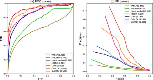
ROC curves and PR curves of all the methods in comparison all the 405 diseases.

Open in new tab Download slide

Table 2

Open in new tab

Average AUC over all the diseases and AUCs of 10 well-characterized disease*

Disease name			AUC
	VADLP	CNNLDA	Ping’s method	SIMCLDA	LDAP	MFLDA	SelMFDF
Breast cancer	0.963	0.886	0.872	0.742	0.830	0.517	0.906
Stomach cancer	0.951	0.928	0.930	0.864	0.928	0.467	0.932
Kidney cancer	0.984	0.981	0.979	0.728	0.977	0.677	0.987
Prostate cancer	0.961	0.932	0.826	0.874	0.710	0.553	0.948
Gastrointestinal system cancer	0.953	0.926	0.896	0.784	0.867	0.582	0.933
Liver cancer	0.978	0.953	0.910	0.799	0.898	0.634	0.943
Hematologic cancer	0.985	0.914	0.908	0.828	0.903	0.716	0.956
Lung cancer	0.981	0.975	0.911	0.790	0.882	0.676	0.963
Ovarian cancer	0.893	0.932	0.913	0.786	0.857	0.558	0.928
Organ system cancer	0.985	0.860	0.950	0.820	0.894	0.747	0.947
Average AUC of 405 diseases	0.969	0.932	0.870	0.745	0.862	0.626	0.900

Disease name			AUC
	VADLP	CNNLDA	Ping’s method	SIMCLDA	LDAP	MFLDA	SelMFDF
Breast cancer	0.963	0.886	0.872	0.742	0.830	0.517	0.906
Stomach cancer	0.951	0.928	0.930	0.864	0.928	0.467	0.932
Kidney cancer	0.984	0.981	0.979	0.728	0.977	0.677	0.987
Prostate cancer	0.961	0.932	0.826	0.874	0.710	0.553	0.948
Gastrointestinal system cancer	0.953	0.926	0.896	0.784	0.867	0.582	0.933
Liver cancer	0.978	0.953	0.910	0.799	0.898	0.634	0.943
Hematologic cancer	0.985	0.914	0.908	0.828	0.903	0.716	0.956
Lung cancer	0.981	0.975	0.911	0.790	0.882	0.676	0.963
Ovarian cancer	0.893	0.932	0.913	0.786	0.857	0.558	0.928
Organ system cancer	0.985	0.860	0.950	0.820	0.894	0.747	0.947
Average AUC of 405 diseases	0.969	0.932	0.870	0.745	0.862	0.626	0.900

*Ten well-characterized diseases are those which are associated with at least 20 lncRNAs. The bold values indicate the higher AUCs.

Table 2

Open in new tab

Average AUC over all the diseases and AUCs of 10 well-characterized disease*

Disease name			AUC
	VADLP	CNNLDA	Ping’s method	SIMCLDA	LDAP	MFLDA	SelMFDF
Breast cancer	0.963	0.886	0.872	0.742	0.830	0.517	0.906
Stomach cancer	0.951	0.928	0.930	0.864	0.928	0.467	0.932
Kidney cancer	0.984	0.981	0.979	0.728	0.977	0.677	0.987
Prostate cancer	0.961	0.932	0.826	0.874	0.710	0.553	0.948
Gastrointestinal system cancer	0.953	0.926	0.896	0.784	0.867	0.582	0.933
Liver cancer	0.978	0.953	0.910	0.799	0.898	0.634	0.943
Hematologic cancer	0.985	0.914	0.908	0.828	0.903	0.716	0.956
Lung cancer	0.981	0.975	0.911	0.790	0.882	0.676	0.963
Ovarian cancer	0.893	0.932	0.913	0.786	0.857	0.558	0.928
Organ system cancer	0.985	0.860	0.950	0.820	0.894	0.747	0.947
Average AUC of 405 diseases	0.969	0.932	0.870	0.745	0.862	0.626	0.900

Disease name			AUC
	VADLP	CNNLDA	Ping’s method	SIMCLDA	LDAP	MFLDA	SelMFDF
Breast cancer	0.963	0.886	0.872	0.742	0.830	0.517	0.906
Stomach cancer	0.951	0.928	0.930	0.864	0.928	0.467	0.932
Kidney cancer	0.984	0.981	0.979	0.728	0.977	0.677	0.987
Prostate cancer	0.961	0.932	0.826	0.874	0.710	0.553	0.948
Gastrointestinal system cancer	0.953	0.926	0.896	0.784	0.867	0.582	0.933
Liver cancer	0.978	0.953	0.910	0.799	0.898	0.634	0.943
Hematologic cancer	0.985	0.914	0.908	0.828	0.903	0.716	0.956
Lung cancer	0.981	0.975	0.911	0.790	0.882	0.676	0.963
Ovarian cancer	0.893	0.932	0.913	0.786	0.857	0.558	0.928
Organ system cancer	0.985	0.860	0.950	0.820	0.894	0.747	0.947
Average AUC of 405 diseases	0.969	0.932	0.870	0.745	0.862	0.626	0.900

*Ten well-characterized diseases are those which are associated with at least 20 lncRNAs. The bold values indicate the higher AUCs.

Table 3

Open in new tab

Average AUPR over all the diseases and AUPRs of 10 well-characterized disease*

Disease name	VADLP	CNNLDA	AUPR Ping’s method	SIMCLDA	LDAP	MFLDA	SelMFDF
Breast cancer	0.624	0.531	0.403	0.047	0.396	0.031	0.569
Stomach cancer	0.372	0.338	0.364	0.138	0.094	0.008	0.327
Kidney cancer	0.238	0.709	0.663	0.030	0.462	0.034	0.722
Prostate cancer	0.370	0.361	0.333	0.176	0.297	0.092	0.358
Gastrointestinal system cancer	0.879	0.782	0.271	0.130	0.238	0.104	0.804
Liver cancer	0.875	0.830	0.498	0.140	0.511	0.110	0.784
Hematologic cancer	0.461	0.425	0.403	0.216	0.370	0.121	0.435
Lung cancer	0.628	0.526	0.437	0.131	0.363	0.171	0.581
Ovarian cancer	0.205	0.394	0.483	0.027	0.427	0.023	0.372
Organ system cancer	0.837	0.781	0.765	0.411	0.628	0.338	0.757
Average AUC of 405 diseases	0.481	0.283	0.152	0.059	0.127	0.039	0.303

Disease name	VADLP	CNNLDA	AUPR Ping’s method	SIMCLDA	LDAP	MFLDA	SelMFDF
Breast cancer	0.624	0.531	0.403	0.047	0.396	0.031	0.569
Stomach cancer	0.372	0.338	0.364	0.138	0.094	0.008	0.327
Kidney cancer	0.238	0.709	0.663	0.030	0.462	0.034	0.722
Prostate cancer	0.370	0.361	0.333	0.176	0.297	0.092	0.358
Gastrointestinal system cancer	0.879	0.782	0.271	0.130	0.238	0.104	0.804
Liver cancer	0.875	0.830	0.498	0.140	0.511	0.110	0.784
Hematologic cancer	0.461	0.425	0.403	0.216	0.370	0.121	0.435
Lung cancer	0.628	0.526	0.437	0.131	0.363	0.171	0.581
Ovarian cancer	0.205	0.394	0.483	0.027	0.427	0.023	0.372
Organ system cancer	0.837	0.781	0.765	0.411	0.628	0.338	0.757
Average AUC of 405 diseases	0.481	0.283	0.152	0.059	0.127	0.039	0.303

^*10 well-characterized diseases are those which are associated with at least 20 lncRNAs.

The bold values indicate the higher AUPRs.

Table 3

Open in new tab

Average AUPR over all the diseases and AUPRs of 10 well-characterized disease*

Disease name	VADLP	CNNLDA	AUPR Ping’s method	SIMCLDA	LDAP	MFLDA	SelMFDF
Breast cancer	0.624	0.531	0.403	0.047	0.396	0.031	0.569
Stomach cancer	0.372	0.338	0.364	0.138	0.094	0.008	0.327
Kidney cancer	0.238	0.709	0.663	0.030	0.462	0.034	0.722
Prostate cancer	0.370	0.361	0.333	0.176	0.297	0.092	0.358
Gastrointestinal system cancer	0.879	0.782	0.271	0.130	0.238	0.104	0.804
Liver cancer	0.875	0.830	0.498	0.140	0.511	0.110	0.784
Hematologic cancer	0.461	0.425	0.403	0.216	0.370	0.121	0.435
Lung cancer	0.628	0.526	0.437	0.131	0.363	0.171	0.581
Ovarian cancer	0.205	0.394	0.483	0.027	0.427	0.023	0.372
Organ system cancer	0.837	0.781	0.765	0.411	0.628	0.338	0.757
Average AUC of 405 diseases	0.481	0.283	0.152	0.059	0.127	0.039	0.303

Disease name	VADLP	CNNLDA	AUPR Ping’s method	SIMCLDA	LDAP	MFLDA	SelMFDF
Breast cancer	0.624	0.531	0.403	0.047	0.396	0.031	0.569
Stomach cancer	0.372	0.338	0.364	0.138	0.094	0.008	0.327
Kidney cancer	0.238	0.709	0.663	0.030	0.462	0.034	0.722
Prostate cancer	0.370	0.361	0.333	0.176	0.297	0.092	0.358
Gastrointestinal system cancer	0.879	0.782	0.271	0.130	0.238	0.104	0.804
Liver cancer	0.875	0.830	0.498	0.140	0.511	0.110	0.784
Hematologic cancer	0.461	0.425	0.403	0.216	0.370	0.121	0.435
Lung cancer	0.628	0.526	0.437	0.131	0.363	0.171	0.581
Ovarian cancer	0.205	0.394	0.483	0.027	0.427	0.023	0.372
Organ system cancer	0.837	0.781	0.765	0.411	0.628	0.338	0.757
Average AUC of 405 diseases	0.481	0.283	0.152	0.059	0.127	0.039	0.303

^*10 well-characterized diseases are those which are associated with at least 20 lncRNAs.

The bold values indicate the higher AUPRs.

Table 4

Open in new tab

Comparison of different methods based on AUC and AUPR with the paired Wilcoxon test

p-value between VADLP and another method	CNNLDA	Ping’s method	SIMCLDA	LDAP	MFLDA	SelMFDF
p-value of AUC	1.5281e-05	2.3362e-05	1.0745e-06	3.2352e-05	3.1702e-07	3.26384e-05
p-value of AUPR	1.1348e-05	0.0002	3.0745e-07	6.3247e-06	1.5643e-06	5.63271e-05

p-value between VADLP and another method	CNNLDA	Ping’s method	SIMCLDA	LDAP	MFLDA	SelMFDF
p-value of AUC	1.5281e-05	2.3362e-05	1.0745e-06	3.2352e-05	3.1702e-07	3.26384e-05
p-value of AUPR	1.1348e-05	0.0002	3.0745e-07	6.3247e-06	1.5643e-06	5.63271e-05

Table 4

Open in new tab

Comparison of different methods based on AUC and AUPR with the paired Wilcoxon test

p-value between VADLP and another method	CNNLDA	Ping’s method	SIMCLDA	LDAP	MFLDA	SelMFDF
p-value of AUC	1.5281e-05	2.3362e-05	1.0745e-06	3.2352e-05	3.1702e-07	3.26384e-05
p-value of AUPR	1.1348e-05	0.0002	3.0745e-07	6.3247e-06	1.5643e-06	5.63271e-05

p-value between VADLP and another method	CNNLDA	Ping’s method	SIMCLDA	LDAP	MFLDA	SelMFDF
p-value of AUC	1.5281e-05	2.3362e-05	1.0745e-06	3.2352e-05	3.1702e-07	3.26384e-05
p-value of AUPR	1.1348e-05	0.0002	3.0745e-07	6.3247e-06	1.5643e-06	5.63271e-05

Fig. 6

The recall values at different top |$k$| cutoffs.

Open in new tab Download slide

The experimental results demonstrated that the contribution of node attributes was the most significant among the three modules. One of the possible reasons is that node attributes embed direct similarities and associations between lncRNAs and diseases and also their neighboring lncRNAs and diseases. Pairwise topology contributed the second most to the results. Compared with node attributes, topological information can be considered as indirect relations between lncRNA and disease, which is hidden in the structure of the heterogeneous graph. Feature distribution encoded from node attributes by VAE is a representation of the underlying relationship between graph nodes, which is latent information. It is an essential component in the prediction model and it can also help with the improvement of prediction performance. In addition, we did investigation of balance controls in imbalanced issues of lncRNA–disease associations, and the statements and experimental results are listed in SF4.

Comparison with other methods

The ROC and PR curves of all the methods in comparison over all the 405 diseases are given in Figure 5. The AUC and AUPR over all the diseases and 10 well-characterized diseases that are associated with at least 20 lncRNAs are given in Tables 2 and 3. As shown by Figure 5A and Table 2, our model achieved the highest average AUC of 0.956, which was 2.4% higher than the 2nd best CNNLDA, 5.6% better than SelMFDF, 8.6% higher than Ping’s method, 9.4% and 21.1% higher than LDAP and SIMCLDA and 33% better than the worst performed MFLDA. In terms of average AUPR over all the diseases, our model achieved the best AUPR of 0.449, which is 16.6%, 14.7%, 29.7%, 39%, 32.2% and 41% higher than that of CNNLDA, SelMFDF, Ping’s method, SIMCLDA, LDAP and MFLDA. For the 10 well-characterized diseases, which are associated with at least 20 lncRNAs, our model achieved the best performance over eight diseases in terms of average AUC and eight diseases with respect to AUPR as shown in Tables 2 and 3. Paired Wilcoxon test results demonstrated that our model statistically significantly (p-value < 0.05) outperformed other methods with respect to both AUC and AUPR as shown in Table 4.

As shown by the results, even though CNNLDA utilizes the neural network, it ignores the feature distribution and attribute information of lncRNA–disease pairwises, so its performance is not as good as our methods. Ping’s method is based on information flow propagation and LDAP is based on SVM, their performance was similar with respect to ROC, PR curve, average AUC and AUPR over all the diseases. One of the possible reasons is that both LDAP and Ping’s method exploited the similarity and association information of lncRNAs and diseases. Without considering intra-lncRNA and disease similarities, SIMCLDA and MFLDA performed much worse than Ping’s method and LDAP. Our method outperformed CNNLDA, Ping’s method and LDAP with the newly introduced pairwise topology, node attributes and deep feature distributions.

Table 5

Open in new tab

The top 15 breast cancer-related lncRNA candidates

Rank	LncRNA name	Source of verification	Rank	LncRNA name	Source of verification
1	PANDAR	Lnc2Cancer, LncRNADisease	9	CCAT2	Lnc2Cancer, LncRNADisease
2	XIST	Lnc2Cancer, LncRNADisease	10	HOTAIR	Lnc2Cancer, LncRNADisease
3	SPRY4-IT1	Lnc2Cancer, LncRNADisease	11	MALAT1	Lnc2Cancer, LncRNADisease
4	ZFAS1	Lnc2Cancer, LncRNADisease	12	MIR124-2HG	Literature
5	LINC-ROR	Lnc2Cancer, LncRNADisease	13	SOX2-OT	Lnc2Cancer, LncRNADisease
6	PVT1	Lnc2Cancer, LncRNADisease	14	LINC-PINT	Literature
7	CCAT1	Lnc2Cancer, LncRNADisease	15	LSINCT5	Lnc2Cancer
8	CDKN2B-AS1	LncRNADisease

Rank	LncRNA name	Source of verification	Rank	LncRNA name	Source of verification
1	PANDAR	Lnc2Cancer, LncRNADisease	9	CCAT2	Lnc2Cancer, LncRNADisease
2	XIST	Lnc2Cancer, LncRNADisease	10	HOTAIR	Lnc2Cancer, LncRNADisease
3	SPRY4-IT1	Lnc2Cancer, LncRNADisease	11	MALAT1	Lnc2Cancer, LncRNADisease
4	ZFAS1	Lnc2Cancer, LncRNADisease	12	MIR124-2HG	Literature
5	LINC-ROR	Lnc2Cancer, LncRNADisease	13	SOX2-OT	Lnc2Cancer, LncRNADisease
6	PVT1	Lnc2Cancer, LncRNADisease	14	LINC-PINT	Literature
7	CCAT1	Lnc2Cancer, LncRNADisease	15	LSINCT5	Lnc2Cancer
8	CDKN2B-AS1	LncRNADisease

Table 5

Open in new tab

The top 15 breast cancer-related lncRNA candidates

Rank	LncRNA name	Source of verification	Rank	LncRNA name	Source of verification
1	PANDAR	Lnc2Cancer, LncRNADisease	9	CCAT2	Lnc2Cancer, LncRNADisease
2	XIST	Lnc2Cancer, LncRNADisease	10	HOTAIR	Lnc2Cancer, LncRNADisease
3	SPRY4-IT1	Lnc2Cancer, LncRNADisease	11	MALAT1	Lnc2Cancer, LncRNADisease
4	ZFAS1	Lnc2Cancer, LncRNADisease	12	MIR124-2HG	Literature
5	LINC-ROR	Lnc2Cancer, LncRNADisease	13	SOX2-OT	Lnc2Cancer, LncRNADisease
6	PVT1	Lnc2Cancer, LncRNADisease	14	LINC-PINT	Literature
7	CCAT1	Lnc2Cancer, LncRNADisease	15	LSINCT5	Lnc2Cancer
8	CDKN2B-AS1	LncRNADisease

Rank	LncRNA name	Source of verification	Rank	LncRNA name	Source of verification
1	PANDAR	Lnc2Cancer, LncRNADisease	9	CCAT2	Lnc2Cancer, LncRNADisease
2	XIST	Lnc2Cancer, LncRNADisease	10	HOTAIR	Lnc2Cancer, LncRNADisease
3	SPRY4-IT1	Lnc2Cancer, LncRNADisease	11	MALAT1	Lnc2Cancer, LncRNADisease
4	ZFAS1	Lnc2Cancer, LncRNADisease	12	MIR124-2HG	Literature
5	LINC-ROR	Lnc2Cancer, LncRNADisease	13	SOX2-OT	Lnc2Cancer, LncRNADisease
6	PVT1	Lnc2Cancer, LncRNADisease	14	LINC-PINT	Literature
7	CCAT1	Lnc2Cancer, LncRNADisease	15	LSINCT5	Lnc2Cancer
8	CDKN2B-AS1	LncRNADisease

Table 6

Open in new tab

The top 15 colorectal cancer-related lncRNA candidates

Rank	LncRNA name	Source of verification	Rank	LncRNA name	Source of verification
1	MEG3	Lnc2Cancer, LncRNADisease	9	CASC2	Lnc2Cancer, LncRNADisease
2	CCAT2	Lnc2Cancer, LncRNADisease	10	CASC19	LncRNADisease
3	GHET1	Lnc2Cancer, LncRNADisease	11	CRNDE	Lnc2Cancer, LncRNADisease
4	HOTAIRM1	Lnc2Cancer, LncRNADisease	12	TP53COR1	LncRNADisease
5	BANCR	Lnc2Cancer, LncRNADisease	13	TUG1	Lnc2Cancer, LncRNADisease
6	LSINCT5	Lnc2Cancer	14	KCNQ1OT1	Lnc2Cancer, LncRNADisease
7	AFAP1-AS1	Lnc2Cancer, LncRNADisease	15	NEAT1	Lnc2Cancer, LncRNADisease
8	HOTAIR	Lnc2Cancer, LncRNADisease

Rank	LncRNA name	Source of verification	Rank	LncRNA name	Source of verification
1	MEG3	Lnc2Cancer, LncRNADisease	9	CASC2	Lnc2Cancer, LncRNADisease
2	CCAT2	Lnc2Cancer, LncRNADisease	10	CASC19	LncRNADisease
3	GHET1	Lnc2Cancer, LncRNADisease	11	CRNDE	Lnc2Cancer, LncRNADisease
4	HOTAIRM1	Lnc2Cancer, LncRNADisease	12	TP53COR1	LncRNADisease
5	BANCR	Lnc2Cancer, LncRNADisease	13	TUG1	Lnc2Cancer, LncRNADisease
6	LSINCT5	Lnc2Cancer	14	KCNQ1OT1	Lnc2Cancer, LncRNADisease
7	AFAP1-AS1	Lnc2Cancer, LncRNADisease	15	NEAT1	Lnc2Cancer, LncRNADisease
8	HOTAIR	Lnc2Cancer, LncRNADisease

Table 6

Open in new tab

The top 15 colorectal cancer-related lncRNA candidates

Rank	LncRNA name	Source of verification	Rank	LncRNA name	Source of verification
1	MEG3	Lnc2Cancer, LncRNADisease	9	CASC2	Lnc2Cancer, LncRNADisease
2	CCAT2	Lnc2Cancer, LncRNADisease	10	CASC19	LncRNADisease
3	GHET1	Lnc2Cancer, LncRNADisease	11	CRNDE	Lnc2Cancer, LncRNADisease
4	HOTAIRM1	Lnc2Cancer, LncRNADisease	12	TP53COR1	LncRNADisease
5	BANCR	Lnc2Cancer, LncRNADisease	13	TUG1	Lnc2Cancer, LncRNADisease
6	LSINCT5	Lnc2Cancer	14	KCNQ1OT1	Lnc2Cancer, LncRNADisease
7	AFAP1-AS1	Lnc2Cancer, LncRNADisease	15	NEAT1	Lnc2Cancer, LncRNADisease
8	HOTAIR	Lnc2Cancer, LncRNADisease

Rank	LncRNA name	Source of verification	Rank	LncRNA name	Source of verification
1	MEG3	Lnc2Cancer, LncRNADisease	9	CASC2	Lnc2Cancer, LncRNADisease
2	CCAT2	Lnc2Cancer, LncRNADisease	10	CASC19	LncRNADisease
3	GHET1	Lnc2Cancer, LncRNADisease	11	CRNDE	Lnc2Cancer, LncRNADisease
4	HOTAIRM1	Lnc2Cancer, LncRNADisease	12	TP53COR1	LncRNADisease
5	BANCR	Lnc2Cancer, LncRNADisease	13	TUG1	Lnc2Cancer, LncRNADisease
6	LSINCT5	Lnc2Cancer	14	KCNQ1OT1	Lnc2Cancer, LncRNADisease
7	AFAP1-AS1	Lnc2Cancer, LncRNADisease	15	NEAT1	Lnc2Cancer, LncRNADisease
8	HOTAIR	Lnc2Cancer, LncRNADisease

Table 7

Open in new tab

The top 15 hepatocellular cancer-related lncRNA candidates

Rank	LncRNA name	Source of verification	Rank	LncRNA name	Source of verification
1	MALAT1	Lnc2Cancer, LncRNADisease	9	MIR17HG	Literature
2	SNHG1	Lnc2Cancer, LncRNADisease	10	PANDAR	Lnc2Cancer, LncRNADisease
3	PCAT1	Lnc2Cancer, LncRNADisease	11	AFAP1-AS1	Lnc2Cancer, LncRNADisease
4	IGF2-AS	Lnc2Cancer, LncRNADisease	12	DBH-AS1	Lnc2Cancer, LncRNADisease
5	MEG3	Lnc2Cancer, LncRNADisease	13	XIST	Lnc2Cancer, LncRNADisease
6	CDKN2B-AS1	LncRNADisease	14	DANCR	Lnc2Cancer, LncRNADisease
7	LINC00974	Lnc2Cancer, LncRNADisease	15	H19	Lnc2Cancer, LncRNADisease
8	GAS5	LncRNADisease

Rank	LncRNA name	Source of verification	Rank	LncRNA name	Source of verification
1	MALAT1	Lnc2Cancer, LncRNADisease	9	MIR17HG	Literature
2	SNHG1	Lnc2Cancer, LncRNADisease	10	PANDAR	Lnc2Cancer, LncRNADisease
3	PCAT1	Lnc2Cancer, LncRNADisease	11	AFAP1-AS1	Lnc2Cancer, LncRNADisease
4	IGF2-AS	Lnc2Cancer, LncRNADisease	12	DBH-AS1	Lnc2Cancer, LncRNADisease
5	MEG3	Lnc2Cancer, LncRNADisease	13	XIST	Lnc2Cancer, LncRNADisease
6	CDKN2B-AS1	LncRNADisease	14	DANCR	Lnc2Cancer, LncRNADisease
7	LINC00974	Lnc2Cancer, LncRNADisease	15	H19	Lnc2Cancer, LncRNADisease
8	GAS5	LncRNADisease

Table 7

Open in new tab

The top 15 hepatocellular cancer-related lncRNA candidates

Rank	LncRNA name	Source of verification	Rank	LncRNA name	Source of verification
1	MALAT1	Lnc2Cancer, LncRNADisease	9	MIR17HG	Literature
2	SNHG1	Lnc2Cancer, LncRNADisease	10	PANDAR	Lnc2Cancer, LncRNADisease
3	PCAT1	Lnc2Cancer, LncRNADisease	11	AFAP1-AS1	Lnc2Cancer, LncRNADisease
4	IGF2-AS	Lnc2Cancer, LncRNADisease	12	DBH-AS1	Lnc2Cancer, LncRNADisease
5	MEG3	Lnc2Cancer, LncRNADisease	13	XIST	Lnc2Cancer, LncRNADisease
6	CDKN2B-AS1	LncRNADisease	14	DANCR	Lnc2Cancer, LncRNADisease
7	LINC00974	Lnc2Cancer, LncRNADisease	15	H19	Lnc2Cancer, LncRNADisease
8	GAS5	LncRNADisease

Rank	LncRNA name	Source of verification	Rank	LncRNA name	Source of verification
1	MALAT1	Lnc2Cancer, LncRNADisease	9	MIR17HG	Literature
2	SNHG1	Lnc2Cancer, LncRNADisease	10	PANDAR	Lnc2Cancer, LncRNADisease
3	PCAT1	Lnc2Cancer, LncRNADisease	11	AFAP1-AS1	Lnc2Cancer, LncRNADisease
4	IGF2-AS	Lnc2Cancer, LncRNADisease	12	DBH-AS1	Lnc2Cancer, LncRNADisease
5	MEG3	Lnc2Cancer, LncRNADisease	13	XIST	Lnc2Cancer, LncRNADisease
6	CDKN2B-AS1	LncRNADisease	14	DANCR	Lnc2Cancer, LncRNADisease
7	LINC00974	Lnc2Cancer, LncRNADisease	15	H19	Lnc2Cancer, LncRNADisease
8	GAS5	LncRNADisease

According to equation (30), the recall rates under different top |$k$| values are given in Figure 6. Our model consistently outperformed other methods at various |$k$| cutoffs due to the learnt pairwise topology, node attributes and feature distribution. The results demonstrated the capacity of the proposed model in screening real disease-related lncRNAs for the top parts of the prediction results. When |$k$| was 30, the highest recall rate of 85.1% was achieved by our model, and the 2nd best 74.6% was obtained by CNNLDA. 68.9% was obtained by Ping’s method which was slightly higher than the fourth ranked LDAP with a rate of 68.5%. When |$k$| was increased from 60 to 120, our model remained the best performed with recall rates of 91%, 92.4% and 94.4%. The second best was CNNLDA with recall rates of 89.5%, 91.3% and 93.5%. LDAP started to outperform Ping’s method but with a marginal improvement. The corresponding recall rates of LDAP were 81.7%, 88.0% and 93.3% while those of Ping’s method were 81.3%, 87.5% and 92.7%. SIMCLDA was consistently worse than CNNLDA, Ping’s method and LDAP with recall rates of 49.3%, 62.9%, 74.4% and 80.3% when |$k$| was between 30 and 120. The lowest recall values were obtained by MFLDA, which were 42.0%, 53.8%, 60.9% and 65.5%.

Case studies: breast cancer, hepatocellular cancer and colorectal cancer

To further demonstrate the capability of the proposed model in discovering the potential lncRNA–disease associations, we performed case studies over breast, hepatocellular and colorectal cancers. For each cancer, we ranked the lncRNA candidates according to their estimated lncRNA–disease association scores in a descending order.

The top 15 ranked candidates for each cancer are given in Tables 5–7. LncRNADisease, Lnc2Cancer databases and published literatures are used to verify and confirm the predicted lncRNA–disease associations. LncRNADisease provides the information about the lncRNAs and their effects on human diseases, which is obtained from the biological experiments and published literatures [45]. Lnc2Cancer is a manually curated database, which records 4989 lncRNA–disease associations between lncRNAs and human cancers obtained from the biological experiments where dysregulation of lncRNA are further manually confirmed [46].

Firstly, among all the 15 top-ranked breast cancer-related lncRNAs by our model (Table 5), 12 of them are verified by LncRNADisease. This result demonstrated that those lncRNA candidates are indeed related with the disease. Twelve of them are confirmed by Lnc2Cancer, which means that they are upregulated or downregulated in breast cancer tissue. In addition, there are two lncRNA candidates, MIR124-2HG and LINC-PINT, verified by literature. MIR124-2HG is supported by recent study showing that decreased MIR124-2HG expression enhances the proliferation of breast cancer cells targeting BECN1 [59, 60]. As shown by another literature, LINC-PINT is apparently downregulated in breast cancer tissue compared with normal tissue [61, 62].

Secondly, the top 15 hepatocellular cancer-related lncRNAs are given in Table 6. Fourteen of them are confirmed by LncRNADisease, which proved their associations with hepatocellular cancer. Thirteen of the top-ranked candidates are found in Lnc2Cancer, where their expression levels in hepatocellular cancer are significantly different from normal tissue. One candidate is supported by the literature, which has abnormal expression in hypocellular cancer [63, 64].

Lastly, among all the top-ranked lncRNA candidates related to colorectal cancer (Table 7), 14 of them are verified by LncRNADisease and 13 of them are proved by Lnc2Cancer database. The case studies further demonstrated the capability of our model in discovering potential lncRNA–disease associations.

Prediction of novel disease-related lncRNAs

In the end, the proposed model is used for the prediction of lncRNA candidates, which are related with the diseases. The top 50 ranked lncRNA candidates predicted by our model are provided in the ST2 to assist the biologists in discovering true novel disease-related lncRNAs in further wet-lab experiments.

Conclusions

In this paper, we proposed a model to adaptively learn and integrate pairwise topology, node attributes and deep feature distribution encoded from multi-sourced data to predict disease-related lncRNAs. A multi-layer heterogeneous graph was constructed to benefit node attribute embedding and pairwise topology extraction by random walks. A framework based on CAE and VAE was constructed for learning and encoding pairwise topology representation, node attribute representation and feature distribution representation. The attention mechanism was proposed to discriminate the contributions of these three representations and adaptively fuse them. Comparison with five recent lncRNA–disease association prediction models and ablation study demonstrated the improved performance of our model in terms of AUC and AUPR. Notably, our model is more powerful in discovering true lncRNA–disease associations and return them as top-ranked candidates as demonstrated by recall rates under different top |$k$| values. Case studies of three cancers further proved the capacity of our model. Our model can be used as a prioritization tool to screen potential candidates and then discover true lncRNA–disease associations through wet laboratory experiments.

Key Points

A new multi-layer heterogeneous graph is proposed to benefit the extraction and representation of diverse relations among multiple sources of data, lncRNAs, diseases and miRNAs, for lncRNA–disease association modeling.
We extract three levels of representations between a pair of lncRNA and disease including the novel node attributes to represent the lncRNA–disease associations, which are inferred via their common lncRNAs, diseases and miRNAs, a new high-level feature distribution to reveal the deep and underlying relations across three sources of data and a pairwise topology to represent the learnt hidden topological structural relations.
An attentional representation-level integration and optimization module is proposed to fuse three levels of representations adaptively.
The contributions of each representation and improved performance were demonstrated by ablation study and comparison with six state-of-the-art lncRNA–disease prediction models over a public dataset. The improved recall rates under different top |$k$| values showed that our model was powerful in discovering true disease-related lncRNAs in the top-ranked candidates. Case studies of three cancers further proved the capacity of the proposed model.

Funding

Natural Science Foundation of China (61972135); Natural Science Foundation of Heilongjiang Province (LH2019F049 and LH2019A029); China Postdoctoral Science Foundation (2019M650069); Heilongjiang Postdoctoral Scientific Research Staring Foundation (BHLQ18104); Fundamental Research Foundation of Universities in Heilongjiang Province for Technology Innovation (KJCX201805); Innovation Talents Project of Harbin Science and Technology Bureau (2017RAQXJ094); Fundamental Research Foundation of Universities in Heilongjiang Province for Youth Innovation Team (RCYJTD201805).

Conflict of interest

The Authors declare that there is no conflict of interest.

Nan Sheng is studying for his master’s degree in the School of Computer Science and Technology at Heilongjiang University, Harbin, China. His research interests include complex network analysis and deep learning.

Hui Cui, PhD (The University of Sydney), is a lecturer at Department of Computer Science and Information Technology, La Trobe University, Melbourne, Australia. Her research interests lie in data-driven and computerized models for biomedical and health informatics.

Tiangang Zhang, PhD (the University of Tokyo), is an associate professor of the Department of Mathematical Science, Heilongjiang University, Harbin, China. His current research interests include complex network analysis and computational fluid dynamics.

Ping Xuan, PhD (Harbin Institute of Technology), is a professor at the School of Computer Science and Technology, Heilongjiang University, Harbin, China. Her current research interests include computational biology, complex network analysis and deep learning.

References

1.

Derrien

T

,

Johnson

R

,

Bussotti

G

, et al.

The GENCODE v7 catalog of human long noncoding RNAs: analysis of their gene structure, evolution, and expression

.

Genome Res

2012

;

22

(

9

):

775

–

1789

.

Google Scholar

Crossref

WorldCat

2.

Guttman

M

,

Rinn

JL

.

Modular regulatory principles of large non-coding RNAs

.

Nature

2012

;

482

(

7385

):

339

–

46

.

3.

Wang

KC

,

Chang

HY

.

Molecular mechanisms of long noncoding RNAs

.

Mol Cell

2011

;

43

(

6

):

904

–

14

.

4.

Wapinski

O

,

Chang

HY

.

Long noncoding RNAs and human disease

.

Trends Cell Biol

2011

;

21

(

6

):

354

–

61

.

5.

Core

LJ

,

Waterfall

JJ

,

Lis

JT

.

Nascent RNA sequencing reveals widespread pausing and divergent initiation at human promoters

.

Science

2008

;

322

:

1845

–

8

.

6.

Esteller

M

.

Non-coding RNAs in human disease

.

Nat Rev Genet

2011

;

12

(

12

):

861

–

74

.

7.

Guttman

M

,

Amit

I

,

Garber

M

, et al.

Chromatin signature reveals over a thousand highly conserved large non-coding RNAs in mammals

.

Nature

2009

;

458

(

7235

):

223

–

7

.

8.

Tsai

MC

,

Manor

O

,

Wang

Y

, et al.

Long noncoding RNA as modular scaffold of histone modification complexes

.

Science

2010

;

329

(

5992

):

689

–

93

.

9.

Chen

X

,

Sun

YZ

,

Guan

NN

, et al.

Computational models for lncRNA function prediction and functional similarity calculation

.

Brief Funct Genomics

2019

;

18

(

1

):

58

–

82

.

10.

Xuan

P

,

Sheng

T

,

Wang

X

, et al.

Inferring disease-associated microRNAs in heterogeneous networks with node attributes

.

IEEE/ACM Trans Comput Biol Bioinform

2018

;

14

(

8

):

1

–

13

.

Google Scholar

OpenURL Placeholder Text

WorldCat

11.

Chen

X

,

Xie

D

,

Zhao

Q

, et al.

MicroRNAs and complex diseases: from experimental results to computational models

.

Brief Bioinform

2019

;

20

(

2

):

515

–

39

.

12.

Mei

JP

,

Kwoh

CK

,

Yang

P

, et al.

Drug-target interaction prediction by learning from local information and neighbors

.

Bioinformatics

2013

;

29

(

2

):

238

–

45

.

13.

Chen

X

,

Yan

CC

,

Zhang

X

, et al.

Drug-target interaction prediction: databases, web servers and computational models

.

Brief Bioinform

2016

;

17

(

4

):

696

–

712

.

14.

Chen

X

,

Ren

B

,

Chen

M

, et al.

NLLSS: predicting synergistic drug combinations based on semi-supervised learning

.

PLoS Comput Biol

2016

;

12

(

7

):

e1004975

.

15.

Gayvert

KM

,

Aly

O

,

Platt

J

, et al.

A computational approach for identifying synergistic drug combinations

.

PLoS Comput Biol

2017

;

13

(

1

):

e1005308

.

Google Scholar

OpenURL Placeholder Text

WorldCat

16.

Chen

X

,

Huang

YA

,

Wang

XS

, et al.

FMLNCSIM: fuzzy measure-based lncRNA functional similarity calculation model

.

Oncotarget

2016

;

7

(

29

):

45948

–

58

.

17.

Xuan

P

,

Jia

L

,

Zhang

T

, et al.

LDAPred: a method based on information flow propagation and a convolutional neural network for the prediction of disease-associated lncRNAs

.

Int J Mol Sci

2019

;

20

(

18

):

4458

.

Google Scholar

Crossref

WorldCat

18.

Chen

X

,

Yan

CC

,

Zhang

X

, et al.

Long non-coding RNAs and complex diseases: from experimental results to computational models

.

Brief Bioinform

2017

;

18

(

4

):

558

–

76

.

Google Scholar

PubMed

OpenURL Placeholder Text

WorldCat

19.

Chen

X

,

Yan

GY

.

Novel human lncRNA-disease association inference based on lncRNA expression profiles

.

Bioinformatics

2013

;

29

(

20

):

2617

–

24

.

20.

Ping

P

,

Wang

L

,

Kuang

L

, et al.

A novel method for lncRNA-disease association prediction based on an lncRNA-disease association network

.

IEEE/ACM Trans Comput Biol Bioinform

2018

;

16

(

2

):

688

–

93

.

21.

Li

Y

,

Li

J

,

Bian

N

.

DNILMF-LDA: prediction of lncRNA-disease associations by dual-network integrated logistic matrix factorization and Bayesian optimization

.

Genes

2019

;

10

(

8

):

608

.

Google Scholar

Crossref

WorldCat

22.

Xuan

Z

,

Li

J

,

Yu

J

, et al.

A probabilistic matrix factorization method for identifying lncRNA-disease associations

.

Genes

2018

;

10

(

2

):

126

.

Google Scholar

Crossref

WorldCat

23.

Zheng

X

,

Ding

H

,

Mamitsuka

H

, et al.

Collaborative matrix factorization with multiple similarities for predicting drug-target interactions

. In:

Proceedings of the 19th ACM SIGKDD International Conference on Knowledge Discovery and Data Mining 2013

, pp.

1025

–

33

, ACM, Chicago Illinois, USA.

OpenURL Placeholder Text

WorldCat

24.

Chen

X

,

You

ZH

,

Yan

GY

, et al.

IRWRLDA: improved random walk with restart for lncRNA-disease association prediction

.

Oncotarget

2016

;

7

(

36

):

57919

–

31

.

25.

Chen

X

.

KATZLDA: KATZ measure for the lncRNA-disease association prediction

.

Sci Rep

2015

;

5

:

16840

.

26.

Ganegoda

GU

,

Li

M

,

Wang

W

, et al.

Heterogeneous network model to infer human disease-long intergenic non-coding RNA associations

.

IEEE Trans Nanobioscience

2015

;

2

(

14

):

175

–

83

.

Google Scholar

OpenURL Placeholder Text

WorldCat

27.

Zhou

M

,

Wang

X

,

Li

J

, et al.

Prioritizing candidate disease-related long non-coding RNAs by walking on the heterogeneous lncRNA and disease network

.

Mol Biosyst

2015

;

11

(

3

):

760

–

9

.

28.

Sun

J

,

Shi

H

,

Wang

Z

, et al.

Inferring novel lncRNA-disease associations based on a random walk model of a lncRNA functional similarity network

.

Mol Biosyst

2014

;

10

(

8

):

2074

–

81

.

29.

Gu

C

,

Liao

B

,

Li

X

, et al.

Global network random walk for predicting potential human lncRNA-disease associations

.

Sci Rep

2017

;

7

(

1

):

12442

.

30.

Zhang

J

,

Zhang

Z

,

Cheng

Z

, et al.

Integrating multiple heterogeneous networks for novel lncRNA-disease association inference

.

IEEE/ACM Trans Comput Biol Bioinform

2017

;

16

(

2

):

396

–

406

.

31.

Lan

W

,

Li

M

,

Zhao

K

, et al.

LDAP: a web server for lncRNA-disease association prediction

.

Bioinformatics

2017

;

33

(

3

):

458

–

60

.

Google Scholar

PubMed

OpenURL Placeholder Text

WorldCat

32.

Ding

L

,

Wang

M

,

Sun

D

, et al.

TPGLDA: novel prediction of associations between lncRNAs and diseases via lncRNA-disease-gene tripartite graph

.

Sci Rep

2018

;

8

(

1

):

1065

.

33.

Yu

J

,

Xuan

Z

,

Feng

X

, et al.

A novel collaborative filtering model for LncRNA-disease association prediction based on the Naive Bayesian classifier

.

BMC Bioinformatics

2019

;

20

(

1

):

396

.

34.

Fan

XN

,

Zhang

SW

,

Zhang

SY

, et al.

Prediction of lncRNA-disease associations by integrating diverse heterogeneous information sources with RWR algorithm and positive pointwise mutual information

.

BMC Bioinformatics

2019

;

20

(

1

):

87

.

35.

Fu

G

,

Wang

J

,

Domeniconi

C

, et al.

Matrix factorization-based data fusion for the prediction of lncRNA-disease associations

.

Bioinformatics

2017

;

34

(

9

):

1529

–

37

.

Google Scholar

Crossref

WorldCat

36.

Lu

C

,

Yang

M

,

Luo

F

, et al.

Prediction of lncRNA-disease associations based on inductive matrix completion

.

Bioinformatics

2018

;

34

(

19

):

3357

–

64

.

37.

Yu

G

,

Wang

Y

,

Wang

J

, et al.

Weighted matrix factorization based data fusion for predicting lncRNA-disease associations

. In:

2018 IEEE International Conference on Bioinformatics and Biomedicine (BIBM) 2018

, pp.

572

–

7

, IEEE, Madrid, Spain.

OpenURL Placeholder Text

WorldCat

38.

Wang

Y

,

Yu

G

,

Domeniconi

C

, et al.

Selective matrix factorization for multi-relational data fusion

. In:

International Conference on Database Systems for Advanced Applications 2019

, pp.

313

–

29

,

Springer, Chiang Mai, Thailand

.

OpenURL Placeholder Text

WorldCat

39.

Xuan

P

,

Cao

Y

,

Zhang

T

, et al.

Dual convolutional neural networks with attention mechanisms based method for predicting disease-related lncRNA genes

.

Front Genet

2019

;

10

:

416

.

40.

Xuan

P

,

Pan

S

,

Zhang

T

, et al.

Graph convolutional network and convolutional neural network based method for predicting lncRNA-disease associations

.

Cell

2019

;

9

(

8

):

1012

.

Google Scholar

OpenURL Placeholder Text

WorldCat

41.

Cen

Y

,

Zou

X

,

Zhang

J

, et al.

Representation learning for attributed multiplex heterogeneous network

. In:

Proceedings of the 25th ACM SIGKDD International Conference on Knowledge Discovery and Data Mining 2019

, pp.

1358

–

68

,

ACM, Anchorage, USA

.

OpenURL Placeholder Text

WorldCat

42.

Liu

M

,

Liu

J

,

Chen

Y

, et al.

AHNG: representation learning on attributed heterogeneous network

.

Inform Fusion

2019

;

50

:

221

–

30

.

Google Scholar

Crossref

WorldCat

43.

Hu

B

,

Fang

Y

,

Shi

C

.

Adversarial learning on heterogeneous information networks

. In:

Proceedings of the 25th ACM SIGKDD International Conference on Knowledge Discovery and Data Mining 2019

, pp.

120

–

9

,

ACM, Anchorage, USA

.

OpenURL Placeholder Text

WorldCat

44.

Chen

X

,

Yu

G

,

Wang

J

, et al.

ActiveHNE: Active Heterogeneous Network Embedding

. In:

28th International Joint Conference on Artificial Intelligence 2019

,

FedAI, Macao, China

.

OpenURL Placeholder Text

WorldCat

45.

Bao

Z

,

Yang

Z

,

Huang

Z

, et al.

LncRNADisease 2.0: an updated database of long non-coding RNA-associated diseases

.

Nucleic Acids Res

2018

;

47

(

D1

):

D1034

–

7

.

Google Scholar

Crossref

WorldCat

46.

Gao

Y

,

Wang

P

,

Wang

Y

, et al.

Lnc2Cancer v2. 0: updated database of experimentally supported long non-coding RNAs in human cancers

.

Nucleic Acids Res

2018

;

47

(

D1

):

D1028

–

33

.

Google Scholar

Crossref

WorldCat

47.

Li

JH

,

Liu

S

,

Zhou

H

, et al.

starBase v2. 0: decoding miRNA-ceRNA, miRNA-ncRNA and protein-RNA interaction networks from large-scale CLIP-Seq data

.

Nucleic Acids Res

2013

;

42

(

D1

):

D92

–

7

.

48.

Huang

Z

,

Shi

J

,

Gao

Y

, et al.

HMDD v3. 0: a database for experimentally supported human microRNA-disease associations

.

Nucleic Acids Res

2018

;

47

(

D1

):

D1013

–

7

.

Google Scholar

Crossref

WorldCat

49.

Jalali

S

,

Bhartiya

D

,

Lalwani

MK

, et al.

Systematic transcriptome wide analysis of lncRNA-miRNA interactions

.

PLoS One

2013

;

2

(

8

):

e53823

.

Google Scholar

OpenURL Placeholder Text

WorldCat

50.

Paraskevopoulou

MD

,

Hatzigeorgiou

AG

.

Analyzing miRNA-lncRNA interactions

.

Methods Mol Biol

2016

;

1402

:

271

–

86

.

51.

Wang

D

,

Wang

J

,

Lu

M

, et al.

Inferring the human microRNA functional similarity and functional network based on microRNA-associated diseases

.

Bioinformatics

2010

;

26

(

13

):

1644

–

50

.

52.

Chen

X

,

Yan

CC

,

Luo

C

, et al.

Constructing lncRNA functional similarity network based on lncRNA-disease associations and disease semantic similarity

.

Sci Rep

2015

;

5

:

11338

.

53.

Wang

F

,

Landau

DP

.

Efficient, multiple-range random walk algorithm to calculate the density of states

.

Phys Rev Lett

2001

;

86

(

10

):

2050

.

54.

Kingma

DP

,

Ba

J

.

Adam: a method for stochastic optimization

In:

3rd International Conference on Learning Representations (ICLR)

2015

, pp. 1–15,

DBLP, San Diego, USA

.

55.

Leonard

J

,

Kramer

MA

.

Improvement of the backpropagation algorithm for training neural networks

.

Comput Chem Eng

1990

;

14

(

3

):

337

–

41

.

Google Scholar

Crossref

WorldCat

56.

Ling

CX

,

Huang

J

,

Zhang

H

.

AUC: a better measure than accuracy in comparing learning algorithms

. In:

Conference of the Canadian Society for Computational Studies of Intelligence 2003

, pp.

329

–

41

,

Springer, Kingston, Canada

.

OpenURL Placeholder Text

WorldCat

57.

Saito

T

,

Rehmsmeier

M

.

The precision-recall plot is more informative than the ROC plot when evaluating binary classifiers on imbalanced datasets

.

PLoS One

2015

;

3

(

10

):

e0118432

.

Google Scholar

OpenURL Placeholder Text

WorldCat

58.

Pahikkala

T

,

Airola

A

,

Pietila

S

, et al.

Toward more realistic drug-target interaction predictions

.

Brief Bioinform

2015

;

16

(

2

):

325

–

37

.

59.

Huang

R

,

Zhang

Y

,

Han

B

, et al.

Circular RNA HIPK2 regulates astrocyte activation via cooperation of autophagy and ER stress by targeting MIR124-2HG

.

Autophagy

2017

;

13

(

10

):

1722

–

41

.

60.

Lv

XB

,

Jiao

Y

,

Qing

Y

, et al.

miR-124 suppresses multiple steps of breast cancer metastasis by targeting a cohort of pro-metastatic genes in vitro

.

Chin J Cancer

2011

;

30

(

12

):

821

–

30

.

61.

Pang

B

,

Wang

Q

,

Ning

S

, et al.

Landscape of tumor suppressor long noncoding RNAs in breast cancer

.

J Exp Clin Cancer Res

2019

;

38

(

1

):

79

.

62.

Zhang

M

,

Zhao

K

,

Xu

X

, et al.

A peptide encoded by circular form of LINC-PINT suppresses oncogenic transcriptional elongation in glioblastoma

.

Nat Commun

2018

;

9

(

1

):

4475

.

63.

Negrini

M

,

Gramantieri

L

,

Sabbioni

SM

, et al.

microRNA involvement in hepatocellular carcinoma

.

Anticancer Agents Med Chem

2011

;

11

(

6

):

500

–

21

.

64.

Zhu

H

,

Han

C

,

Wu

T

.

MiR-17-92 cluster promotes hepatocarcinogenesis

.

Carcinogenesis

2015

;

36

(

10

):

1213

–

22

.

This article is published and distributed under the terms of the Oxford University Press, Standard Journals Publication Model (https://dbpia.nl.go.kr/journals/pages/open_access/funder_policies/chorus/standard_publication_model)

Download all slides

Month:	Total Views:
May 2020	88
June 2020	39
July 2020	50
August 2020	39
September 2020	24
October 2020	37
November 2020	35
December 2020	41
January 2021	29
February 2021	15
March 2021	20
April 2021	42
May 2021	18
June 2021	55
July 2021	36
August 2021	21
September 2021	32
October 2021	69
November 2021	50
December 2021	36
January 2022	36
February 2022	33
March 2022	26
April 2022	50
May 2022	35
June 2022	19
July 2022	24
August 2022	22
September 2022	22
October 2022	34
November 2022	20
December 2022	15
January 2023	3
February 2023	41
March 2023	16
April 2023	28
May 2023	57
June 2023	33
July 2023	20
August 2023	30
September 2023	45
October 2023	53
November 2023	69
December 2023	65
January 2024	65
February 2024	53
March 2024	58
April 2024	28
May 2024	45
June 2024	32
July 2024	69
August 2024	32
September 2024	45
October 2024	26
November 2024	32
December 2024	30
January 2025	22
February 2025	30
March 2025	24
April 2025	27
May 2025	10

Article Contents

Attentional multi-level representation encoding based on convolutional and variance autoencoders for lncRNA–disease association prediction

Abstract

Introduction

Materials and Methods

Dataset

Triple-layer heterogeneous graph

Pairwise topology extraction by random walk

Heterogenous node attributes extraction by embedding strategy

Multi-level knowledge encoding

Pairwise topology encoding by CAE

Node attribute encoding by CAE

Feature distribution representation and encoding by VAE

Attentional multi-level representation integration and optimization

Experimental results and discussions

Experimental setup and evaluation metrics

Ablation experiments

Comparison with other methods

Case studies: breast cancer, hepatocellular cancer and colorectal cancer

Prediction of novel disease-related lncRNAs

Conclusions

Funding

Conflict of interest

References

Citations

Views

Altmetric

Email alerts

Citing articles via

Latest

Most Read

Most Cited

Article Contents

Attentional multi-level representation encoding based on convolutional and variance autoencoders for lncRNA–disease association prediction Free

Abstract

Introduction

Materials and Methods

Dataset

Triple-layer heterogeneous graph

Pairwise topology extraction by random walk

Heterogenous node attributes extraction by embedding strategy

Multi-level knowledge encoding

Pairwise topology encoding by CAE

Node attribute encoding by CAE

Feature distribution representation and encoding by VAE

Attentional multi-level representation integration and optimization

Experimental results and discussions

Experimental setup and evaluation metrics

Ablation experiments

Comparison with other methods

Case studies: breast cancer, hepatocellular cancer and colorectal cancer

Prediction of novel disease-related lncRNAs

Conclusions

Funding

Conflict of interest

References

Citations

Views

Altmetric

Email alerts

Citing articles via

Latest

Most Read

Most Cited

This Feature Is Available To Subscribers Only

Attentional multi-level representation encoding based on convolutional and variance autoencoders for lncRNA–disease association prediction