


Abstract
Motivation: Calculating the frequency of occurrence of each substring of length k in DNA sequences is a common task in many bioinformatics applications, including genome assembly, error correction, and sequence alignment. Although the problem is simple, efficient counting of datasets with high sequencing depth or large genome size is a challenge. Results: We propose a robust and efficient method, CHTKC, to solve the k-mer counting problem with a lock-free hash table that uses linked lists to resolve collisions. We also design new mechanisms to optimize memory usage and handle situations where memory is not enough to accommodate all k-mers. CHTKC has been thoroughly tested on seven datasets under multiple memory usage scenarios and compared with Jellyfish2 and KMC3. Our work shows that using a hash-table-based method to effectively solve the k-mer counting problem remains a feasible solution.
Introduction
K-mer counting refers to extracting each substring of length k from a given number of DNA sequences and calculating its frequency of occurrence, which is a preliminary step in many bioinformatics applications. De novo genome assembly algorithms often construct a De Bruijn graph using k-mers [1]. The k-mer frequencies can be used to correct sequencing errors in reads, taking advantage of the fact that error k-mers often have low frequencies [2]. K-mer counting can also improve the computational efficiency of sequence alignment [3]. High sequencing depth and/or large genome sizes often lead to large numbers of DNA sequences. With limited resources (memory and disk space) available on most computers, efficiently performing k-mer counting on such data sets is a challenge.
K-mers can be easily generated by using many existing tools, such as Pse-in-One [4] and BioSeq-Analysis [5, 6]. Various data structures and algorithms have been employed to solve the k-mer counting problem. Jellyfish [7] uses a hash table, BFCounter [8] and Turtle [9] use bloom filters, and KCMBT [10] uses burst trees. KAnalyze [11] uses a modified external merge sort algorithm to deal with the limited memory. To further reduce memory usage and increase the computational efficiency, many disk-based methods have also been proposed, such as DSK [12], MSPKmerCounter [13], KMC2 [14], and Gerbil [15]. These tools use a two-stage processing scheme, first all k-mers are divided into groups and stored on disk, and then each group is processed separately using a sorting algorithm or hash tables. Among them, KMC3 [16] has been proven to be quite successful, but it still has some limitations. It is difficult to evenly divide k-mers into groups using minimizers (or signatures), and it requires additional task scheduling algorithms to handle each group when using a multi-threaded environment. For large data sets, the distribution stage can involve significant I/O costs. Since data sets usually have different characteristics, it is difficult to determine the minimum memory required to handle the largest group with high performance, and it is not possible to further effectively utilize the larger available memory. In addition, for high-depth data sets, compared to the use of a hash table, the sort-based strategy may require more computation time in terms of finding entries.
These limitations make us review the more intuitive solution using a hash table. Jellyfish’s implementation uses an open addressing method to resolve collisions, which requires a lower load factor to ensure good performance. In addition, when memory is low, its merge strategy can be very time consuming. These disadvantages may cause Jellyfish to perform worse than disk-based methods, even with higher memory usage.
We propose a method CHTKC to solve the problem of k-mer counting. CHTKC uses a lock-free hash table, which uses chaining to resolve collisions. This has many advantages over open addressing. Lock-free technology is essential for good performance when accessing a single hash table through multiple threads.
CHTKC uses a strategy different from Jellyfish when memory is not enough to accommodate all k-mers. CHTKC will first fill all pre-allocated memory. After that, it attempts to compress the k-mers that do not exist in memory and temporarily stores them on disk. After the original data are completely processed, the compressed k-mers on the disk do not overlap with the k-mers in memory and are treated as another batch of sequence data. The hash table can be reused to calculate new data. This process continues until no more temporary data are generated.
Sequencing errors in the raw data often lead to the fact that the total number of k-mers is greater than the size of the genome. However, because sequence data are retrieved randomly, errors are also randomly distributed among the sequence data. Therefore, if the number of pre-allocated entries in memory is close to the size of the genome, most of the k-mers counted in the first batch are correct, and most of the k-mers temporarily stored on disk are errors. Since an error k-mer always has a very low frequency, using this method can make the temporary data as small as possible, which means that subsequent batches can be processed in an acceptable time.
We also propose a memory-optimized version of CHTKC, which can pre-allocate up to 4G entries. In practice, if memory is tight or the genome size of the target organism is less than 4G, the optimized version is recommended, which is practical for processing general human data sets.
Methods
Encoding of k-mers
A k-mer is essentially a sequence of characters, and each character can only be one of A, C, G, or T. In order to reduce the memory and storage usage of k-mers and improve computing efficiency, k-mers should be encoded as binary bits. We encode A as 00, C as 01, G as 10, and T as 11. Therefore, a 64-bit unsigned integer can hold a k-mer with a maximum length of 32, and a longer k-mer requires more than one unsigned integer to store.
Since a read sequence can come from either strand of a particular genomic location, we calculate each k-mer in its canonical form, which is defined as the lexicographically smaller of the k-mer and its reverse complement [14]. For example, the canonical form of the k-mer sequence ACGGT is ACCGT.
Counting k-mers using a chaining hash table
CHTKC uses a hash table to solve the k-mer counting problem (Figure 1). A hash table is essentially a large array of buckets in which key-value entries can be stored. For the k-mer counting problem, the keys and values correspond to the k-mer sequence and its frequency of occurrence, respectively.
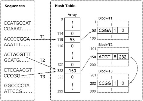
Hash table structure. In this example, the length of the bucket array is 400. In total, 300 nodes (load factor 0.75) are pre-allocated and assigned to three threads T1, T2, and T3 in blocks. Each thread can read different parts from the original sequencing data and add k-mers in parallel. For T1 and T2, they are inserting k-mers that do not yet exist in the hash table. Each of T1 and T2 requests a new node from its own block and inserts the corresponding k-mer into its target bucket. For T3, the k-mer CCGG that it is inserting conflicts with the ACGT that T2 has just inserted, so the new node must be linked to the tail of the node that contains ACGT.
Other data structures, such as lists or trees, can also store key-value entries. The most common operation is to find the entry using the key provided. In a list or tree, entries must be compared one by one through a path, which means that more there are entries more the comparison operations involved. However, in a hash table, the location of an entry is calculated by the hash function using the key itself, and comparisons occur only when there are collisions. Therefore, when many key-value entries are frequently operated, which is the case of the k-mer counting problem, using a hash table can achieve better performance.
Using the hash function, an entry can be found with |$\mathrm{O}(1)$| time complexity. However, because the index is calculated directly from the keys, two different keys may be mapped to the same index value, that is, they are in the same bucket, which is called collision. To handle any unexpected patterns in the k-mer distribution, CHTKC sets the length of the bucket array |$L$| to a prime number to ensure that the number of collisions is as small as possible [17].
Open addressing (used by Jellyfish) and chaining are two primary methods used to resolve collisions. Although using open addressing can save memory for a single entry, it requires a lower load factor (ratio of number of entries to bucket array length) to achieve good performance compared to using the chaining method, which means lower memory utilization. In CHTKC, we use chaining to resolve collisions, which links all entries mapped to the same bucket to each other.
Figure 1 illustrates our hash table implementation scheme. The bucket array only stores the address of the first node of its collision list (or NULL if no k-mers are inserted into the bucket). Each node contains three fields: the k-mer sequence, its frequency of occurrence, and the address of the next node in the list. When a k-mer is inserted into the hash table, its target bucket index is calculated using the hash function; then, CHTKC will iterate each node in the bucket following the links. If a node containing the same k-mer is found, the count field of the node will be incremented by 1; otherwise, a new node with the k-mer sequence and an initial count value of 1 will be linked at the tail of the list.
Inserting k-mers in a lock-free manner
Since K-mer counting is a time-consuming task, it usually requires the use of multi-threaded parallel technology. Locks are often used to prevent shared resources from being accessed by multiple threads simultaneously to avoid race conditions. However, the most used shared resource is the hash table itself. If it can only be updated serially, the multi-core CPU cannot be effectively used. By allocating a separate lock for each bucket, using finer granularity can improve multi-threaded performance. Although this sounds feasible, it requires additional memory cost.
Like Jellyfish, we use compare-and-swap (CAS) operations to implement the lock-free feature of the hash table. The CAS operation is performed like a simple function taking three parameters: a memory location, an old value, and a new value. It compares the current value of the memory location with the old value, which was obtained earlier and may have already been modified by another thread. If these values are equal, the memory location is updated to the new value provided; otherwise, the operation fails. The atomicity of CAS operations is guaranteed by hardware.
Algorithm 1 describes the k-mer insertion algorithm used in CHTKC. Since the CAS algorithm is designed to execute atomically on only one operation step, the node containing the k-mer should be prepared before inserting into the list to prevent accidental modification by other threads. CHTKC first assumes that the k-mer needs a new node, it requests a new node and initializes it with the k-mer and a frequency value of 1 (lines 1–4). Then, the index of the k-mer’s target bucket is calculated using the hash function, and the collision list is found (lines 5–6). CHTKC iterates through each node in the list (lines 8–17), and if a node containing the same k-mer is found, the CAS operation is used to increase the frequency value of the node by 1 (lines 10–15). If the iteration has reached the tail of the list, the node can be inserted into the list using the CAS operation. If the operation fails, it indicates that the tail has been modified by other threads and the list will be iterated again (lines 7–18).
Insert a new k-mer into the hash table
| Input: The hash table array T, and the new k-mer M |
| 1: N ← request an available node |
| 2: Nk-mer ← M |
| 3: Ncount ← 1 |
| 4: Nnext ← NULL |
| 5: i ← hashFunc(M) |
| 6: L ← Ti |
| 7: repeat |
| 8: P ← Lhead |
| 9: while P ≠ NULL do |
| 10: if Pk-mer = M then |
| 11: repeat |
| 12: C ← Pcount |
| 13: until CAS (Pcount, C, C + 1) = True |
| 14: mark N reusable and return |
| 15: end if |
| 16: P ← Pnext |
| 17: end while |
| 18: until CAS(P, NULL, N) = True |
Memory-related optimizations
CHTKC needs to specify the amount of memory to be used in advance, and then it uses a predefined load factor to allocate memory to the hash table array and nodes. K-mer counting is a memory-consuming task, especially for species such as human with huge genome sizes. In these cases, memory is usually insufficient, so nodes should be allocated as much as possible, that is, the load factor should be as large as possible. However, as the load factor increases, the hash table performance decreases, so a load factor of 0.75 is chosen as a good balance. This is another advantage over open addressing. For open addressing, the hash table consists of actual nodes, which means that when the load factor is equal to 0.75, 25% of the nodes are wasted. In CHTKC, the hash table contains only pointers to nodes, which takes up less memory than the actual nodes, so it wastes less memory, especially when counting for longer k-mers.
An extra pointer field is introduced for each node by the chaining method, so it requires additional memory usage, but it can be optimized. For example, when counting k-mers shorter than 32 bp, 8 bytes (a 64-bit unsigned integer) are used to encode a k-mer; 4 bytes would usually be enough to hold the k-mer frequency value, but the compiler also needs to align the node with address boundaries. In this example, the compiler adds additional padding of 4 bytes (which holds nothing and is wasted) to the frequency value field; thus, the node consumes 16 bytes of memory in total. Although some instructions can be used to force the compiler to pack the node without padding, accessing structures with address boundaries unaligned will negatively affect performance.
In the example above, if the node contains a pointer field, it will require an extra 8 bytes, which will increase memory usage by 50%. A pointer is essentially an index of a large memory unit array. A pointer with 8 bytes can address 264 nodes, which is a huge space. In practice, if the number of nodes to be allocated is less than 4G (232), a 32-bit unsigned integer instead of a pointer can be used for indexing. In this case, the nodes need to be stored in a single array no larger than 232, and the first node is reserved as an invalid state (like a NULL pointer). Then, the addressing operation of the nodes can be done using the index of the array, which involves little additional computational cost. In this way, the memory usage of the hash table array is reduced by 50%, and the 32-bit index occupies the padding introduced by the compiler alignment, so that the memory usage of a node is still equal to 16 bytes, without the padding being wasted or the performance impacted (Figure 2).
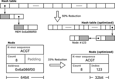
This example illustrates RAM optimization when counting k-mers shorter than 32 bp. By replacing memory addresses with indexes of the node array, both the nodes and hash table array are reduced in size.
The k-mer counting process workflow
CHTKC uses a reading thread and a writing thread to handle I/O operations (I/O threads); other threads are used to handle k-mers (computing threads). A read buffer and a write buffer are adopted for transferring data between I/O threads and computing threads. Buffers are also shared resources; locks are used to achieve synchronization in our implementation. Data are transferred in blocks, which reduces the rate of transmission.
Using the predefined memory usage and load factor, the number of nodes and the length of the hash table array can be determined. CHTKC does not dynamically allocate nodes when needed by the thread, but uses a single array to pre-allocate all nodes and divides these nodes into separate blocks (Figure 1). Each block is assigned to a thread, and the thread preferentially obtains new nodes from its own block to avoid contention. If a thread cannot obtain new nodes from other blocks, after one thread runs out of nodes, other threads must immediately stop acquiring new nodes to ensure the synchronization of the algorithm, which will result in a waste of a certain number of nodes. In our implementation, each thread makes polling requests for all blocks, starting from its own block, until it cannot get nodes from any block. This ensures that contention occurs only after most nodes have been used, and very few nodes are wasted due to synchronization. As with updating the hash table, CAS operations are used to ensure good performance.
CHTKC starts by reading raw sequences from disk, and data are transferred in blocks and enqueued into buffers. Each computing thread acquires a block from the read buffer and extracts each k-mer from the sequences. When the nodes are not exhausted, k-mers are always successfully inserted into the hash table. Otherwise, those k-mers that are not in the hash table are temporarily moved to disk and processed in subsequent batches. CHTKC compresses consecutive k-mers into longer super k-mers instead of storing each k-mer separately to save disk space and I/O costs (Figure 3). After all the raw sequences have been processed, the task of counting k-mers in the hash table has been completed, and these k-mers are exported to disk as part of the result. The super k-mers do not overlap with those in the hash table, so they are treated as another batch of sequences to be processed. Then, the hash table is cleared and the next batch of counting tasks is performed on these super k-mers. CHTKC repeats this process until it no longer produces any super k-mer. The result is a concatenation of the results of each batch of counting tasks.
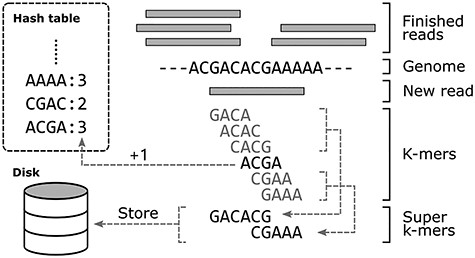
This example of counting 4-mers illustrates how CHTKC compresses k-mers after nodes are exhausted. Among the 6 k-mers extracted from the new 9 bp read GACACGAAA, only ACGA exists in the hash table, and other k-mers need to be temporarily stored to disk. The first three consecutive k-mers are compressed to GACACG, and the last two are compressed to CGAAA.
Another benefit is related to the strategy of pre-allocating nodes. Normally, when exporting hash table entries to disk, each collision list needs to be iterated. Since adjacent linking nodes are unlikely to be in nearby memory areas, accessing such a linked list will result in many cache misses. In CHTKC, nodes are stored in arrays, so they can be iterated by accessing consecutive memory units, and CHTKC will benefit greatly from the cache system. This is useful when filtering out many entries when exporting to disk, such as filtering out k-mers that only appear once.
Results
CHTKC was compared with Jellyfish2 [7] and KMC3 [16] on seven datasets with different genome sizes and sequencing depths, and tested with the following four k values: 28, 40, 55, and 65. The tests were run on a server equipped with two Intel Xeon E5-2650 v2 CPUs (8 cores each at 2.60 GHz), 192 GB RAM, and 48 TB HDD (373 MB/s). Each test was run using 32 threads (virtual core number) for best performance.
The Fragaria vesca, Gallus gallus, Musa balbisiana, and three Homo sapiens datasets were previously used in the KMC paper, we also add another deeply sequenced Fraxinus mandshurica dataset (BioProject accession PRJNA512114) to demonstrate the effect of sequencing depth on the results. In our tests, all three tools excluded k-mers that only appeared once, because most of these k-mers are caused by errors. Table 1 shows the statistics of depth of k-mers (the ratio of the total number of k-mers to the number of unique k-mers) that appear at least twice, which basically reflects the sequencing depth and other characteristics of the data sets. The comparison results are shown in Tables 2–4 and Supplementary Tables S1–S4 including execution time (in seconds), memory usage (in GB), and disk usage (in GB).
K-mer depth statistics of the datasets used in the experiment
| Dataset | Genome length | K-mer depth | |||
|---|---|---|---|---|---|
| k = 28 | k = 40 | k = 55 | k = 65 | ||
| F. vesca | 214 | 14 | 11.7 | 9.8 | 9.1 |
| G. gallus | 1043 | 21.5 | 17.3 | 12.6 | 9.8 |
| M. balbisiana | 493 | 42.5 | 32.2 | 23.8 | 19.3 |
| F. mandshurica | 867 | 162.1 | 132.4 | 110.8 | 100.7 |
| H. sapiens 1 | 2943 | 30.7 | 24.9 | 19.7 | 16.9 |
| H. sapiens 2 | 2943 | 35.6 | 27.3 | 19.4 | 14.9 |
| H. sapiens 3 | 2943 | 143.1 | 114.9 | 88.4 | 71.3 |
Note: Genome lengths are in Mbases.
K-mer counting results for the M. balbisiana dataset
| Method | k = 28 | k = 40 | k = 55 | k = 65 | ||||||||
|---|---|---|---|---|---|---|---|---|---|---|---|---|
| RAM | Disk | Time | RAM | Disk | Time | RAM | Disk | Time | RAM | Disk | Time | |
| Jellyfish2 | 19 (500M) | 0 | 847 | 28 (500M) | 0 | 1087 | 40 (500M) | 0 | 1011 | 49 (500M) | 0 | 1343 |
| Jellyfish2 | 82 (9G) | 0 | 1385 | 70 (5G) | 0 | 3859 | 53 (4G) | 0 | 1147 | 63 (3G) | 0 | 1028 |
| KMC3 | 54 | 45 | 387 | 54 | 36 | 433 | 54 | 29 | 420 | 54 | 26 | 418 |
| KMC3 | 41 | 45 | 468 | 41 | 36 | 426 | 41 | 29 | 379 | 41 | 26 | 395 |
| CHTKC | 51 | 0 | 329 | 51 | 0 | 309 | 51 | 0 | 271 | 51 | 0 | 256 |
| CHTKC-opt | 51 | 0 | 314 | 51 | 0 | 306 | 51 | 0 | 267 | 51 | 0 | 240 |
Note: Timings in seconds and RAM/disk consumption in GB.
K-mer counting results for the F. mandshurica dataset
| Method | k = 28 | k = 40 | k = 55 | k = 65 | ||||||||
|---|---|---|---|---|---|---|---|---|---|---|---|---|
| RAM | Disk | Time | RAM | Disk | Time | RAM | Disk | Time | RAM | Disk | Time | |
| Jellyfish2 | 19 (500M) | 0 | 2095 | 28 (500M) | 0 | 2042 | 40 (500M) | 0 | 2007 | 94 (500M) | 0 | 2396 |
| Jellyfish2 | 157 (18G) | 0 | 1472 | 134 (10G) | 0 | 8988 | 101 (8G) | 0 | 1443 | 123 (6G) | 0 | 1503 |
| KMC3 | 103 | 126 | 1198 | 102 | 108 | 1285 | 103 | 98 | 1212 | 103 | 93 | 1254 |
| KMC3 | 53 | 126 | 1131 | 54 | 108 | 1220 | 54 | 98 | 1151 | 53 | 93 | 1353 |
| CHTKC | 100 | 0 | 852 | 100 | 0 | 869 | 100 | 0 | 821 | 100 | 0 | 862 |
| CHTKC-opt | 100 | 0 | 843 | 100 | 0 | 836 | 100 | 0 | 809 | 100 | 0 | 808 |
Note: Timings in seconds and RAM/disk consumption in GB.
K-mer counting results for the H. sapiens 3 dataset
| Method | k = 28 | k = 40 | k = 55 | k = 65 | ||||||||
|---|---|---|---|---|---|---|---|---|---|---|---|---|
| RAM | Disk | Time | RAM | Disk | Time | RAM | Disk | Time | RAM | Disk | Time | |
| Jellyfish2 | 123 (3G) | 251 | 16,766 | 103 (3G) | 492 | 20,468 | 152 (3G) | 636 | 22,372 | 183 (3G) | 670 | 24,886 |
| Jellyfish2 | 157 (18G) | 0 | 12,478 | 137 (10G) | 369 | 53,046 | 104 (8G) | 636 | 23,023 | 125 (6G) | 662 | 20,096 |
| KMC3 | 151 | 596 | 5481 | 151 | 477 | 5716 | 151 | 389 | 5411 | 151 | 343 | 5408 |
| KMC3 | 102 | 596 | 4909 | 102 | 477 | 5262 | 102 | 389 | 4789 | 102 | 343 | 5020 |
| CHTKC | 149 | 19 | 4975 | 149 | 29 | 5205 | 149 | 40 | 4492 | 149 | 75 | 4420 |
| CHTKC-opt | 149 | 19 | 4499 | 149 | 24 | 4482 | 149 | 30 | 3734 | 149 | 38 | 3687 |
Note: Timings in seconds and RAM/disk consumption in GB.
Jellyfish2 cannot be specified with a fixed running memory, it requires an initial size of the hash table as input and expands this size by consuming more memory during execution. We designed two sets of inputs to test Jellyfish2. In the first group, the hash table size is equal to or slightly larger than the genome size of the corresponding organism, and in the other group, the hash table size is much larger.
Of the three tools, Jellyfish2 is the slowest on all datasets. Overall, increasing the initial hash table size improves running speed. However, it is observed that when k was 40, the performance on most data sets was abnormally degraded. We also found that Jellyfish2 cannot scale to use all available memory, probably because it requires the size of the hash table to be an exponential power of 2, which indicates that its hash table strategy is not efficient. When memory is low, Jellyfish2 also generates disk usage, in which case its overall runtime increases significantly, and sometimes even higher than KMC3, which indicates that the disk strategy it uses is not efficient.
KMC3 and CHTKC can both be specified with a fixed running memory, but they are completely different algorithms from the basic architecture. KMC3 is designed to optimize for small memory, while CHTKC attempts to utilize as much memory as possible to speed up the entire process. Therefore, we tested KMC3 and CHTKC under multiple memory usage scenarios for a more comprehensive comparison (Figures 4 and 5 and Supplementary Figures S1–S5).
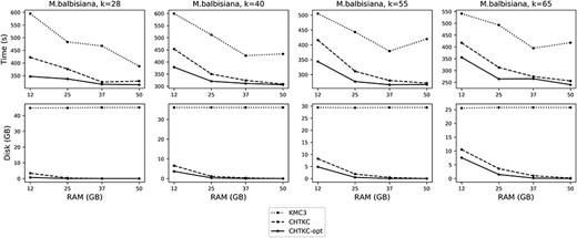
Comparison of KMC3 and CHTKC on the M. balbisiana dataset.
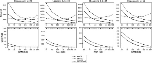
Comparison of KMC3 and CHTKC on the H. sapiens 3 dataset.
Overall, increasing the memory usage improves the performance of both programs. However, the memory scheduling strategy used in Linux systems will inhibit the increase in speed. To reduce I/O operations on the disk, the system uses physical memory to cache the disk contents. For k-mer counting tools, disk operations include reading raw data and writing temporary data. When processing large sequencing data, if the software consumes too much memory or generates a large amount of temporary data, it will cause the system to frequently perform I/O operations, and the software is often interrupted, resulting in performance degradation.
From the results, we found that CHTKC has a better scalability in memory usage than KMC3, because KMC3 usually achieves the best performance with smaller random access memory (RAM, the memory usage), while CHTKC achieves the best performance with a much larger RAM. Therefore, for a fair comparison, we list two sets of KMC3 results in each table, one using the same RAM as CHTKC, and the other using the RAM at which KMC3 performs well on all k values.
The comparisons between KMC3 and CHTKC show that although KMC3 has achieved good performance when using smaller RAM, further increases in RAM cannot bring many benefits. This is because KMC3 distributes all k-mers to disk in the first stage, which is an I/O intensive operation and cannot benefit from the increase of the RAM. Since the temporary data written in the first stage will not change, the increase in memory usage will cause the Linux system to suppress its running speed. For CHTKC, with a larger RAM, the hash table can handle more entries in memory, which directly benefits from the increase in RAM. In addition, its disk usage decreases as memory usage increases, so it will not be severely suppressed by the Linux system.
The results show that CHTKC has advantages in processing high sequencing depth data. The memory on the testing server is sufficient to process the first four datasets, where KMC3 outperforms CHTKC on the F. vesca dataset with the smallest genome size and the lowest sequencing depth. For the G. gallus, which is also a low-depth dataset, CHTKC does not have much advantage. But CHTKC performs much better than KMC3 on the high-depth M. balbisiana and F. mandshurica datasets.
For the H. sapiens datasets, because the number of error k-mers increases with the increase in sequencing depth, the memory is almost always insufficient (Supplementary Table S5), and a larger value of k will cause the number of allocated nodes to decrease, further tightening the memory. CHTKC usually requires at least two batches to process all data (Supplementary Table S6). In these three human datasets, although more than five batches need to be performed on the H. sapiens 3 with the highest sequencing depth, the optimized version of CHTKC outperforms KMC3 with only 100 GB of memory.
The results also show the performance of CHTKC with and without memory optimizations. Because the optimized version can allocate more nodes (Supplementary Table S5), its overall performance is better. We also need to mention that for the optimized version, the upper limit of the number of k-mers that can be stored in memory is 4G, which means that further increase in memory usage will not effectively improve the overall performance. However, if enough memory can be provided, using the normal version can further make full use of memory because it does not have a limit on the number of allocated nodes. In addition, the scalability of the two versions of CHTKC in the number of threads and the length of k-mers is given in Supplementary Figures S6 and S7.
Conclusion
The k-mer counting problem is useful in many bioinformatics applications, such as genome assembly, sequence alignment, remote homology detection of proteins, and folding recognition. As the price of sequencing technology decreases, sequencing data with high depth can be easily obtained, and sequencing data for organisms with huge genome sizes may increase. Therefore, it is an important issue to effectively count k-mers for data having such characteristics.
KMC3 uses a two-stage scheme to reduce memory usage, grouping and distributing k-mers to disk, and then counting by a sorting algorithm. However, for large data sets, the disk space generated in the first stage is large. In addition, the maximum memory usage is determined by the largest group, which means that performance will not improve even if more memory is provided. The advantages of KMC3 are obvious when dealing with low-depth data or memory constraints.
A hash table is well suited for parallel computing because it can be accessed in a lock-free manner. The hash function can quickly find entries with a specific k-mer, which has advantages over sorting methods and can process deep sequencing data faster. When the memory is enough, the hash table can process as many k-mers as possible in the memory and takes up almost no disk space, thereby avoiding the process of extracting k-mers twice. Using the hash table can make full use of memory and has good scalability.
As demonstrated in our tests, several implementations in Jellyfish2 are inefficient. CHTKC is much faster than Jellyfish2 and outperforms KMC3 for datasets with high sequencing depths. It also has better scalability in memory usage than the other two methods. This shows that CHTKC as a hash table-based method is more reasonable and robust, and the hash table is still an ideal data structure to solve the k-mer counting problem.
Conflict of Interest statement
None declared.
K-mer counting is an important task in bioinformatics applications, such as genome assembly. CHTKC solves the problem with a lock-free hash table that uses linked lists to resolve collisions.
CHTKC uses some optimization mechanisms to reduce memory usage and improve running speed.
When insufficient memory causes temporary disk usage, CHTKC uses a new mechanism to process data in batches, which works well with the hash table.
Testing with seven datasets, we demonstrated that CHTKC is a robust and effective method.
Funding
National Natural Science Foundation of China [61771165]; International Postdoctoral Exchange Fellowship [20130053]; China Postdoctoral Science Foundation [2018T110302 and 2014M551246].
Jianan Wang is currently a PhD student at School of Computer Science and Technology, Harbin Institute of Technology. His research interests are machine learning and bioinformatics.
Su Chen is an associate professor at State Key Laboratory of Tree Genetics and Breeding, Northeast Forestry University. His research interests are plant genetics and Genomics.
Lili Dong is currently a PhD student at School of Computer Science and Technology, Harbin Institute of Technology. Her research interests are machine learning and bioinformatics.
Guohua Wang is a professor at School of Computer Science and Technology, Harbin Institute of Technology. He is also a principal investigator at Key Laboratory of Tree Genetics and Breeding, Northeast Forestry University. His research interests are bioinformatics, machine learning and algorithms.
Jianan Wang and Su Chen wish it to be known that, in their opinion, the first two authors should be regarded as the joint First Authors.
