


Abstract
To understand tumor heterogeneity in cancer, personalized driver genes (PDGs) need to be identified for unraveling the genotype–phenotype associations corresponding to particular patients. However, most of the existing driver-focus methods mainly pay attention on the cohort information rather than on individual information. Recent developing computational approaches based on network control principles are opening a new way to discover driver genes in cancer, particularly at an individual level. To provide comprehensive perspectives of network control methods on this timely topic, we first considered the cancer progression as a network control problem, in which the expected PDGs are altered genes by oncogene activation signals that can change the individual molecular network from one health state to the other disease state. Then, we reviewed the network reconstruction methods on single samples and introduced novel network control methods on single-sample networks to identify PDGs in cancer. Particularly, we gave a performance assessment of the network structure control-based PDGs identification methods on multiple cancer datasets from TCGA, for which the data and evaluation package also are publicly available. Finally, we discussed future directions for the application of network control methods to identify PDGs in cancer and diverse biological processes.
Introduction
Genetic mutation, gene amplification and chromosomal rearrangement and transposable elements are genetic mechanisms that drive cancer progression and identity, providing an explanation for oncogene activation [1–3]. Most of researchers have recognized that during tumor progression, the majority of detected altered genes are passengers that do not contribute to oncogenic process but a small fraction of genomic and transcriptomic altered genes are known as driver genes that modify transcriptional programs and therefore drive and sustain tumor progression [4–6]. However, tumor heterogeneity differs in survival fitness, invasive potential and adaptability to the tumor microenvironment and has been the primary obstacle to understanding the functional importance of driver genes in personalized therapies [7–9]. Through recent advances in genomics technologies, comprehensive genomics and proteomics platforms including The Cancer Genome Atlas (TCGA) [10], Cancer Cell Line Encyclopedia (CCLE) [11, 12], Catalogue of Somatic Mutations in Cancer (COSMIC) [13], International Cancer Genome Consortium (ICCG) [14] and Gene Expression Omnibus (GEO) [15] have provided multi-domains of data for understanding the inter-tumor heterogeneity in cancer. The integrative and comparative analyses of these publicly available data lead to an advancement of systematic methods for precision medicine by stratifying patients for targeted therapy. In the past decades, researchers have shifted the focus from the driver gene identification in large cohorts [16–22] to identification of driver genes for individuals—that is personalized driver genes (PDGs) [23–28].
For the driver gene identification in large cohorts, many approaches have provided clues about how genetic driver genes are linked to the complex diseases. To the best understanding, we categorized these approaches into three groups according to their major features. (i) Mutation frequency-based methods, these methods identify the driver genes by finding significantly mutated genes whose mutation rates are significantly higher than the background mutation rate [29, 30]. However, due to the tumor heterogeneity, constructing a reliable background mutation model is difficult, which limits the performance of frequency-based methods. (ii) Machine learning-based methods, these methods are usually trained by using mutations designed as pathogenic or neutral, whose advantage is that such models can be developed for any specific tasks dependent on the available training data but are limited in a few applications due to the probable incompleteness of their cited databases [16–18, 31]. (iii) Network or pathway-based methods, these methods usually assume that cancer is a complex disease with many changes altered at the biological network level [19–22, 32]. Although these methods have been successfully used for prioritizing driver genes in cancer, the human interactome map is often incomplete and error prone because it is built based on the large-scale mixed experimental data rather being cell-type specific, tissue specific or condition specific. Thus developing an integrative framework by incorporating information-rich datasets at multiple omics levels, such as genomic, transcriptomic as well as epigenomic into the improved knowledge of the human interactome, would provide a more comprehensive catalog of prioritizing driver genes at the network or pathway level.
Aiming to offer personalized ways of diagnosis or treatment (i.e. individual patients may have different compositions of driver genes), PDG prediction is required for discovering rare causal events in cancer, which may provide important information for selecting effective therapies [5, 33]. With the development of network science, network analysis and pathway enrichment analysis may provide an informative mechanism of understanding PDGs [34, 35]. In fact, several techniques such as the directed network-based methods (e.g. Single-Sample Controller Strategy (SCS) [23], DawnRank [28] and Paradigm-Shift [24]) and the undirected network-based methods (i.e. HIT’nDRIVE [25], OncoIMPACT [26] and PRODIGY [27]) have been proposed to identify the PDGs. Although these methods could theoretically help investigators select putative driver genes that would have potential for clinical applications [36], we still lack a comprehensive perspective to identify the PDGs for individuals. Recently, structure-based network control approaches have enabled us to investigate how to control the complex networks by using a minimum set of the driver nodes, which could enhance us to understand the network mechanism of the disease progression [23, 37–44].
For the structure-based network control methods, a minimum number of driver nodes that needs to be identified drives the network state from the initial state to desired state depending on the adequate knowledge of the network structure. So far, studies of exploiting the structure-based network control can be primarily divided into two categories according to the network style: (i) focusing on the directed networks [45–53] and (ii) focusing on the undirected networks [54–56]. However, these existing structure-based network control methods cannot be directly applied to the PDGs analysis. This is primarily due to a gap between network control theory and PDGs identification. The rate-limiting step of applying network control methods for PDGs recognition is how to reconstruct the personalized state transition networks that capture the phenotypic transitions between normal and disease states for each individual. To give a comprehensive perspective of applying network control principles toward the PDGs identification at individual patient scale, in this review we first introduced the cancer data resources and formulated the network control problem to identify each individual PDGs. Then, we demonstrated a number of efficient computational techniques for connecting structure-based network control and PDGs identification through reconstructing the personalized state transition networks on single samples, along with the summary of structure-based network control methods. Thirdly, we assessed the performance of structure control-based methods of PDGs identification on 13 cancer datasets from TCGA, for finding the advantages and effectiveness of network control methods of identifying PDGs in practice. In addition, we provided the data and evaluation pipeline which implements the single sample network construction methods and the network control methods for detecting PDGs in cancer. Finally, we discussed the future directions for identifying PDGs in diverse studies and applications adhering to certain network control methods.
Data resources
Through recent advances in genomics technologies, comprehensive genomics and proteomics platforms provide many data resources for identifying the PDGs [57, 58]. For example the success of the TCGA project has led to characterization of over 20 000 primary cancer and matched normal samples spanning 33 cancer types, providing an important opportunity in evaluating the biological relevance of cancer genomics discovery [13]. The CCLE project provides public access to genomic data, analysis and visualization for over 1457 cell lines [11, 12]. The COSMIC is the largest source of expert manually curated somatic mutation information relating to human cancers which combines knowledge data manually curated by experts and genome-wide screen data [59]. The cBio Cancer Genomics Portal (cBioPortal) is an open-access resource for interactive exploration of multidimensional cancer genomics datasets and currently provides access to data of more than 5000 tumor samples from about 20 cancer studies [60]. ICCG aims to catalog genomic abnormalities in tumors from 50 different cancer types, defining the unique genetic signature of an individual tumor type [14]. The GEO repository at the National Center for Biotechnology Information represents the largest public repository of microarray data [15]. GEO currently stores about 112 752 public series submitted directly by 19 692 laboratories, comprising of 3 027 904 samples derived from more than 1600 organisms. In conclusion, these data resources have provided multi-domains of data for the development of computational methods and tools that can efficiently detect PDGs.
To perform comparison across different computational methods, dozens of gene annotation resources are collected due to their prominent roles in the genetics and genomics communities. For example, BioGPS is an online gene annotation resource for enabling users to easily aggregate data on a gene from more than 150 external sources and to personalize their gene report using BioGPS layouts [61]. However, BioGPS does not provide the source gene list for gene annotation which is not easy for users to annotate the enrichment result of a large number of samples. To perform a more systematic method comparison, a list of prior-known driver genes from the Cancer Census Genes (CCG) is usually used as gold standard [62] and also as a proxy for potential drivers to assess the precision of the predicted drivers genes. In addition, CCG is part of COSMIC [59], and it contains mutations of different forms (e.g. gene amplifications, single nucleotide variation, translocations, etc.) that are experimentally validated as driver genes for different cancer types. The Network of Cancer Genes (NCG) is a manually curated repository containing 2372 genes whose somatic modifications have known or predicted cancer driver roles. These genes are collected from 275 publications, including 2 sources of known cancer genes and 273 cancer sequencing screens of more than 100 cancer types from 34 905 cancer donors and multiple primary sites [63]. Although CCG and NCG can provide efficient driver genes list for pan-cancer datasets, they cannot provide cancer-specific driver genes (CSD) for different types. DisGeNET is a discovery platform containing one of the largest publicly available collections of genes and variants associated to human diseases [64]. The DisGeNET dataset contains 628 685 gene–disease associations of 17 549 genes and 24 166 diseases, disorders, traits and clinical or abnormal human phenotypes, which provide an efficient resource for finding different cancer-specific genes. Totally, these data resources have provided multi-domains of data for the development of computational methods and tools that can help systematically exploring the genomic, epigenomic and transcriptomic characteristics of PDGs for individual patients. In Table 1, we gave a summary of the available data sources including personalized samples resources and gene annotation resources for identifying PDGs.
Summary of the available data sources including the personalized samples resources and gene annotation resources for identifying PDGs
| Datasets | Description | Website | References |
|---|---|---|---|
| Resources of personalized samples | |||
| TCGA | Characterization of over 20 000 primary cancer and matched normal samples spanning 33 cancer types | http://cancergenome.nih.gov | [13] |
| GEO | A public functional genomics data repository supporting MIAME-compliant data submissions | https://www.ncbi.nlm.nih.gov/geo/ | [15] |
| COSMIC | The largest source of expert manually curated somatic mutation information relating to human cancers | http://cancer.sanger.ac.uk/cosmic | [59] |
| CCLE | A public access to genomic data, analysis and visualization for over 1457 cell lines | https://portals.broadinstitute.org/ccle/ | [11, 12] |
| cBioPortal | An open-access resource for interactive exploration of multidimensional cancer genomics datasets | http://www.cbioportal.org | [60] |
| ICCG | A resource for functional roles of mutations | https://icgc.org | [14] |
| Resources of gene annotations | |||
| CCG | Mutations of different forms that were experimentally validated as driver genes for different cancer types | https://cancer.sanger.ac.uk/census/ | [59] |
| BioGPS | An online gene annotation resource for enabling users to easily aggregate data on a gene from more than 150 external sources. | http://biogps.gnf.org | [61] |
| NCG | A list of 2372 cancer genes including 711 known cancer genes and tumor suppressor or oncogene annotations from 273 manually curated publications. | http://ncg.kcl.ac.uk/ | [63] |
| DisGeNET | A platform containing one of the largest publicly available collections of genes and variants associated to human diseases. | http://www.disgenet.org/ | [64] |
Problem formulation for network control-based PDGs identification
where x∈RN and y∈RN° respectively denote the gene state and observable gene state at time t in an individual system; |$\mathbf{A}\in {R}^{N\times N}$| and |$\mathbf{C}\in {R}^{N_O\times N}$| respectively represent the state transition matrix and output matrix; |$\mathbf{B}\in {R}^{N\times {N}_C}$| characterizes the driving by NC controllers with the genes. The ‘controllers’ in network control can produce the input signals to make the state transition of the whole network. As in many cases, it is assumed that one driver node can be altered by one independent input signal [68–74]. The element Bij is nonzero if the j-th input signal directly acts on node vi. The output and input matrices are set as |${\mathbf{C}}^T=\Big[\mathbf{I}\Big({c}_1\Big),\mathbf{I} \Big({c}_2\Big),\dots, \mathbf{I}\Big({c}_{N_O}\Big)\Big]$| and |${\mathbf{B}}^T=\Big[\mathbf{I}\Big({b}_{k_1}\Big),\mathbf{I} \Big({b}_{k_2}\Big),\dots, \mathbf{I}\Big({b}_{k_T}\Big)\Big]$|, respectively; |$\Big\{{\mathrm{c}}_1,{c}_2,\dots, {c}_{N_O}\Big\}$| and |$\Big\{{b}_1,{b}_2,\dots, {b}_{N_C}\Big\}$| are the index of the set of observable genes O and constrained control genes U, respectively; |$\mathbf{I}(i)$|denotes the i-th column of the |$N\times N$| identity matrix I.

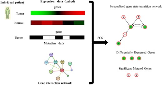
Network control problem to identify PDGs. We assume that each patient has a personalized state transition network during cancer progression in which each edge denotes a pair of interacted genes, while the principles of the personalized network dynamics are unknown. The personalized state transition network is defined as a directed or undirected graph in which each edge denotes the significant interaction difference of gene pairs between the normal state and the tumor state. The network control problem for identifying PDGs is formed as how we can select a feasible subset of network nodes (PDGs) from the personalized state transition network, which can be injected through oncogene activations, to nudge a complex, nonlinear individual system from normal state to disease state. The PDGs may be oncogene activated or drug activated. If the PDGs are activated by oncogene signals, the system state will be changed from a normal state to a disease state. Meanwhile, if the PDGs are drug-activated, the system state should change from disease state to normal state.
Considering the gene expression profiles in normal and tumor samples as the respective state of a given patient, network control tools aim to detect a small number of altered genes by the input signals related with the state transition of individual patient depending on adequate knowledge of the network structure. The PDGs are the altered nodes/genes by the input signals which can make the state transition of the whole biological network. The input signals may be oncogene activation signals such as genetic mutation, gene amplification, chromosomal rearrangement or transposable elements. The ‘controllers’ in network control problem for identifying PDGs mean the genetic or environment factors which produce the oncogene activation signals.
As noted, the state transition of a system from the disease state to the normal state also can be handled when the input signals include drug activations or similar indications (Figure 1). These PDGs can also be efficient sources of drug targets for drug discovery and drug repositioning [75–78].
Obviously, applying network control methods for PDGs identification needs two key steps. One is to construct the personalized state transition networks which are involved in the state transition during disease development for each patient. Another is to design the optimal network control methods based on the structure of personalized state transition networks. Therefore, we will give the detailed discussions on how to apply network control tools for identifying PDGs from such two respects below.
Reconstruction of the personalized state transition network
The personalized state transition network represents which gene pairs are involved in the disease development for each patient. Because the principles of the personalized network dynamics are hidden, it is important to reconstruct the personalized state transition networks with the personalized genetic data (e.g. expression profiles). The ability to unravel the dynamic nature of gene regulation during a biological process is a key challenge in systems biology. Most of the studies for exploiting gene regulation, such as the Gene Network Reconstruction tool [79], the dynamic cascaded method [80], the HotNet2 [21] and the local Bayesian network [81], can describe only the dynamic gene regulation for population samples, and they are not suitable for an individual patient. Some researchers have recognized that most of the currently available methods do not adequately account for heterogeneity in the number of mutations expected by chance. Consequently, they yield many false-positive calls, particularly in cancers with high mutation rates [82–84]. Thus, it is urgently to develop more efficient methods to discover gene regulations or dysfunctional regulations for individuals in a network manner. This section will introduce several techniques to search for the personalized state transition networks (Table 2), including SCS [23], Linear Interpolation to Obtain Network Estimates for Single Samples (LIONESS) [85], Single-Sample Network (SSN) [86], Paired-Single-Sample Network (Paired-SSN) [87] and VarWalker [88].
Summary of different methods to construct the personalized state transition networks
| Methods | Description | Software website | Year | Reference |
|---|---|---|---|---|
| SCS | Include the significant mutated genes and the differential expressed genes and the frequently interrupted interactions in directed gene interaction network | http://sysbio.sibcb.ac.cn/cb/chenlab/software.htm | 2018 | [23] |
| VarWalker | Include mutation genes and their close interactions in undirected gene interaction network | http://bioinfo.mc.vanderbilt.edu/VarWalker.html | 2014 | [88] |
| SSN | Construct an individual-specific network based on statistical perturbation analysis of tumor sample against a group of given control samples | http://sysbio.sibcb.ac.cn/cb/chenlab/software.htm | 2016 | [86] |
| LIONESS | Model regulatory network changes over time and to characterize the regulatory processes active in individual samples. | None | 2019 | [85] |
| Paired-SSN | The differential coexpression network between normal sample network and tumor sample network for each patient | None | 2019 | [87] |
Overview of SCS to identify a personalized state transition network. For the gene expression data and gene mutation profiles (SNP and CNV) for individual patient, SCS identifies the differentially expressed genes and extracted the mutation genes and their close interactors as the personalized state transition network using the RWR algorithm and a randomization-based test in the directed gene interaction network.
To provide a guide and comparison for selecting a reasonable method for reconstructing the personalized state transition networks, we grouped the above approaches into two categories according to the features of used datasets.
(i) Mutation data-based methods (i.e., VarWalker and SCS)
These methods include mutation genes and their close interactors for each sample in the human gene interaction network. VarWalker [88] first assesses the mutation probabilities of all human genes by fitting them to a generalized additive model based on the patient- or sample-specific mutational profile. Then the Random Walker with Restart (RWR) method is executed for each sample to search for interactions among the filtered mutation genes in the human interactome. Finally, VarWalker introduces a randomization-based test to evaluate the candidate interactors by utilizing multiple topologically matched random networks which form the personalized state transition networks.
SCS [23] first identifies the differential expression genes by calculating the log2 fold-change of gene expression between the paired tumor and normal samples. A significance of ±1 is used to indicate the differentially expressed genes for each patient. Then both the mutation genes and their interactors are extracted from each patient by using the RWR algorithm for each patient. Finally, the individual mutation genes, the individual Differentially Expressed Genes method (DEGs) and the interactors are formed as the personalized state transition networks (Figure 2).
(ii) Bulk gene expression data-based methods (i.e., LIONESS, SSN and Paired-SSN)
These methods reconstruct the personalized state transition networks in the bulk gene expression data of tumor samples. LIONESS [85] does not rely upon differential analysis between the tumor sample and a group of normal samples but reconstructs the individual specific network in a population of tumor samples as the personalized state transition networks for each tumor sample. LIONESS constructs the personalized state transition networks by calculating the edge statistical significance between all the tumor samples and the tumor samples without a given single sample. Furthermore, LIONESS can use multiple aggregate network reconstruction techniques for constructing single sample network including Pearson correlation coefficient (PCC) [89], Passing Attributes between Networks for Data Assimilation (PANDA) [90], Mutual Information (MI) [91] and Context Likelihood of Relatedness (CLR) [92].
SSN [86] is a statistical method to construct an individual-specific network solely based on expression data of a single sample, rather than the aggregated network for a group of samples, based on statistical perturbation analysis of a single sample against a group of given control samples. In particular, the SSN method quantifies the individual-specific network of each sample against a group of given control samples in terms of statistical significance in an accurate manner. The SSN needs to have expression data for a group of normal samples, which serve as the reference samples. By using this group of samples, SSN firstly constructs the co-expression network by PCCs and then adds the single sample to the reference samples for constructing the perturbed network. Thus, the SSN method can construct the personalized state transition networks by quantifying the differential network between the reference and perturbed networks. To more precisely demonstrate the regulatory mechanism of the personalized state transition networks, SSN usually uses the protein interaction network to filter the noise of PCC between gene pairs. Note that, SSN method constructs actually a differential co-expression network between groups of normal and a single disease sample [93–97], and the advantage of SSN is that it gives a mathematical criterion to evaluate whether the edge is differential significantly or not. It can also be generalized to other calculation of edge relationship methods, such as conditional mutual inclusive information [98] and Part MI [99] and Partial MI [100].
For the Paired-SSN method [87], the co-expression network of the tumor sample network and normal sample network for each patient is constructed based on statistical perturbation analysis of one sample against a group of given reference samples (e.g. choosing the normal samples data of all of the patients as the reference data here) with the SSN method [86]. In addition, the P-value of an edge for the tumor sample or normal sample also can be obtained by using the SSN method. All of the edges with significant differential correlations (e.g., P-value <0.05) were used to constitute the normal sample network or tumor sample network. Then, the personalized differential co-expression network can be constructed in which edges exist if the P-value of the gene pairs is less than (greater than) 0.05 in the tumor network but greater than (less than) 0.05 in the normal network for each patient. Note that by using Paired-SSN, the protein interaction network is also usually used to filter the noise of co-expression network of the tumor sample network or normal sample network. Finally, personalized state transition networks can be obtained, whose edges are those existing in both the gene interaction network and personalized differential co-expression network for each patient (Figure 3).
![Overview of using the Paired-SSN to construct the personalized state transition network. First, select all of the normal data as the reference data, and construct the tumor network and normal network based on the reference data with the SSN method [86]. Then, construct the single sample network with SSN, in which edges are those existing in both the gene–gene interaction network and the co-expression network for each sample. Finally, construct the personalized state transition network in which the edge between gene i and gene j exists if the P-value of the edge is less than (greater than) 0.05 in the tumor network, but greater than (less than) 0.05 in the normal network.](https://oup.silverchair-cdn.com/oup/backfile/Content_public/Journal/bib/21/5/10.1093_bib_bbz089/7/m_bbz089f3.jpeg?Expires=1750181400&Signature=CVUN-sop~mumYM4hSsmRlRh1ktCWGGtoFTxCvQDlL8TOqKoCKW8syzKqfmFIQ6uOS7iMcevdSyQIBK-MBiEbFAVasPFj9vA~Us9A~3bZPvvYXcD9YrzuvzTdrAMcYFP6dtj3VU7JB1Fa~gH6x85X7I5~s7S8TTj3u-1UeH~o85pOx9jCMu9la~RnyRPDrlnHMGXxn8aON0Dbnjf47Fevz4kK2jdTbeZUZNNEPoQRfOgFdf3-HwydVQKx~IRYIK3pyt7vhi6gfMIVDlKTTGlA2c7HQDbAU4KRm5OProFGK8Zb71xPKc-j7XhKiPGbYWjVUGQ5y7v-jmAsspePFWxrXw__&Key-Pair-Id=APKAIE5G5CRDK6RD3PGA)
Overview of using the Paired-SSN to construct the personalized state transition network. First, select all of the normal data as the reference data, and construct the tumor network and normal network based on the reference data with the SSN method [86]. Then, construct the single sample network with SSN, in which edges are those existing in both the gene–gene interaction network and the co-expression network for each sample. Finally, construct the personalized state transition network in which the edge between gene i and gene j exists if the P-value of the edge is less than (greater than) 0.05 in the tumor network, but greater than (less than) 0.05 in the normal network.
The SSN and Paired-SSN methods quantify the individual-specific network against a group of given control samples in terms of statistical significance of PCC in an accurate manner. Both SSN and Paired-SSN need a group of normal samples in terms of expression data, which serve as the reference samples. The SSN constructs the personalized state transition networks based on statistical perturbation analysis of a tumor sample against a group of given reference samples while the Paired-SSN method constructs personalized state transition networks based on statistical differential analysis of the normal sample network and tumor sample network. Therefore compared with LIONESS method, SSN and Paired-SSN consider more information of individual patients and are suitable for identifying the PDGs of individual cancer patients.
Summary of different structure-based control methods including MMS-based control methods (i.e. full control, target control and constrained target control), MDS-based control method and FVS-based control methods (i.e. DFVS and NCUA)
| Methods | Categories | Targeted states | Network Styles | Dynamics | Year | Reference |
|---|---|---|---|---|---|---|
| MMS-based full controllability | MMS control | Any | Directed | Local nonlinear | 2011 | [52] |
| MMS-based target controllability | MMS control | Any | Directed | Local nonlinear | 2014 | [101,102] |
| MMS-based constrained target controllability | MMS control | Any | Directed | Local nonlinear | 2017 | [49] |
| MDS | MDS control | Any | Undirected | Nonlinear | 2012 | [55] |
| DFVS | FVS control | Attractors | Directed | Nonlinear | 2017 | [53] |
| NCUA | FVS control | Attractors | Undirected | Nonlinear | 2019 | [87] |
Design of the structure-based network control methods
The control process usually is determined by an intrinsic structure and dynamic propagation. Although we have adequate knowledge of the underlying wiring diagram, we lack knowledge of the specific functional forms for biological systems [53]. Analyzing such complicated systems requires the concepts and approaches of structure-based control, which can be used to investigate the controllability of complex networks through a minimum set of driver nodes, even though the edge weights are precisely unknown. Table 3 summarizes the differences among the various Maximum Matching Sets (MMS)-based control methods, including full control, target-control, constrained target control, Minimum Dominating sets (MDSs)-based control method and Feedback Vertex Sets (FVSs)-based control methods. This comparison makes the structure-based control concepts and methods easier to understand. These tools may give a specific view of the network control properties of a system with linear or nonlinear dynamics, which are introduced in detail as follows.
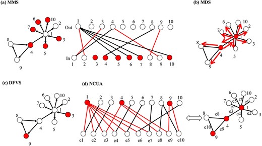
Demonstration of the structure-based control methods. (A) Demonstration of MMS-based control method (full control). MMS-based control method can identify the unmatched nodes {v3,v4,v5,v6,v7,v10} (red nodes) on the right side of the bipartite graph transferred from the directed network, as the driver nodes. (B) Demonstration of MDS-based control method. The network is structurally controllable by selecting an MDS {v1,v4} because each dominated node has its own control signal. (C) Demonstration of DFVS. For DFVS algorithm, the controllability is determined by the FVS {v9} and the source nodes of the network {v3}. (D) Demonstration of NCUA. The NCUA assumes that the edges of the undirected networks are modeled as the bidirected edges. NCUA first constructs a bipartite graph from the original undirected network, in which the nodes of the top side are the nodes of the original graph, and the nodes of the bottom side are the edges of the original graph. Then, it determines the MDS of the top-side nodes {v1,v4,v9} to cover the bottom-side nodes in the bipartite graph using ILP. The red nodes in (A–D) are the driver nodes identified by MMS, MDS, DFVS and NCUA, respectively.
When Equation (4) is satisfied, the system in Equation (3) is structurally controllable. Note that the maximum in Equation (4) implies that given the input and output matrices B and C, we need to choose the proper nonzero weights in A to satisfy Equation (4)—that is when|${N}_O=N,{N}_C=N$|, both |$\Big\{{\mathrm{c}}_1,{c}_2,\dots, {c}_{N_O}\Big\}$| and |$\Big\{{b}_1,{b}_2,\dots, {b}_{N_C}\Big\}$| are all of the nodes in the network, and the controllability is the full controllability [52]. The full controllability concerns the ability to drive the state of all of the nodes of the network to their desired values by selecting driver nodes from all of the nodes. Thus, when |${N}_C=N$|,|$\Big\{{b}_1,{b}_2,\dots, {b}_{N_C}\Big\}$| are all of the nodes of the network, and the controllability is the output controllability or the target controllability [101, 102]. This target controllability aims to control the state of the target nodes by choosing driver nodes from all of the nodes. In contrast, the objective of constraint target controllability (CTC) is to control the state of target nodes by choosing driver nodes only from the set of constrained control nodes (i.e. the candidate driver nodes) [49]. The CTC can be viewed as a more general framework than full controllability [52] or target controllability [102]. So far, this kind of structure-based network control approach has been applied widely to analyze the mechanism of biological networks in diverse fields [103–107]. In Figure 4A, we intuitively explained how the MMS-based method (full control) can be used to analyze the controllability of complex networks.
The second type is the MDS-based control methods. It is another important model for the controllability of dynamic networks. Nacher and Akutsu [55] introduced the MDS method to the controllability study for undirected networks by assuming that each edge in a network is bidirectional, and they showed that a network is structurally controllable by selecting the nodes in the MDS as the driver nodes (Figure 4B). Nacher and Akutsu [55] observed that only driver nodes in the MMS model can be controlled directly through external signals, whereas each driver node in the MDS model can control its associated edges independently. Furthermore, each non-driver node is controllable if it is at least adjacent to a driver node. The MDS-based model may lead to the identification of important nodes for the control of networks [55]. It also has been recognized that the MDS model is capable of controlling an undirected network, by assuming that each node in the MDS can control all of its outgoing edges separately [55, 108]. Despite its success and widespread application in searching for the important genes in the protein interaction network [107, 109–112], the MDS-based model may be more expensive, because each driver node controls its outgoing links independently and thus more powerful control is required (Figure 4B).
where each constrained condition is set for each edge in E. Then the noted ILP can be used to perform the FVS calculation in the directed network.
where xi will take the value 1 when node i belongs to the dominating cover set; the objective is to obtain the minimum number of nodes in |${V}_{\mathrm{T}}$| to cover all the nodes in |${V}_{\perp }$|.
For FVS-based control methods, including DFVS and NCUA, the optional solution can be obtained efficiently for moderate sizes of graphs with up to a few tens of thousands of nodes by utilizing an algorithm that applies the classic branch and bound method [121, 122] to determine an optimal solution, although the search for FVS is a non-deterministic polynomial-hard problem. Figure 4C and D illustrates the corresponding processes of DFVS and NCUA to discover the driver nodes, respectively.
In fact, the target control of complex networks is usually useful for the practical application in biological networks [102, 103]. However, as seen from the above discussions, MDS-based control method and FVS-based control methods (DFVS and NCUA) focus on the full control of networks. That is they assume the observable nodes O and constrained control nodes U are the whole network nodes. Therefore, in the future, for more actual control purpose in biological networks it will be necessary to introduce the target control [102, 103] and constrained target control [104] into MDS-based control method and FVS-based control methods.
Performance assessment of the structure control-based PDGs identification methods
According to the requirement of network control principles, normal–disease paired samples needed to be obtained. That is each individual should have paired samples (i.e. a normal sample and a tumor sample). To demonstrate the usage of the structure control principles, we used those cancer datasets that contain sufficient number of normal–disease paired samples (>20 paired samples) in TCGA for case study here. By searching TCGA, we found 13 cancer datasets which can meet the requirements. In Table 4, we gave a summary of the sample information including the number of normal samples, tumor samples and paired samples in all 33 cancer datasets of TCGA.
where |$\mu (S)$| and |$\delta (S)$| are the mean and standard variance of the PCC absolute value distribution S of all gene pairs, respectively.
To keep the edge direction and filter the noise of PCC correlation in the personalized state transition networks, the directed protein interaction network was also used on the LIONESS and SSN and Paired-SSN, which was obtained from the literature [28] by integrating multiple types of datasets, including Mutual Exclusivity Modules in cancer [123, 124], Reactome [125], NCI-Nature Curated PID [126] and Kyoto Encyclopedia of Genes and Genomes [127]. The directed protein interaction network consists of 11 648 proteins and 211 794 edges, including self-loops within the network to account for auto-regulation events.
Summary of the sample information including the number of normal samples, tumor samples and paired samples in all 33 TCGA cancer datasets
| Abbreviations | Full name | Number of normal samples | Number of tumor samples | Number of paired samples |
|---|---|---|---|---|
| LAML | Acute myeloid leukemia | 0 | 151 | 0 |
| ACC | Adrenocortical carcinoma | 0 | 79 | 0 |
| BLCA | Bladder urothelial carcinoma | 19 | 413 | ≤19 |
| LGC | Breast lobular carcinoma | 0 | 529 | 0 |
| BRCA | Breast ductal carcinoma | 113 | 1102 | 112 |
| CESC | Cervical carcinoma | 3 | 304 | ≤3 |
| CHOL | Cholangiocarcinoma | 9 | 36 | ≤9 |
| COAD | Colorectal adenocarcinoma | 50 | 478 | 50 |
| ESCA | Esophageal carcinoma | 11 | 161 | ≤11 |
| GBM | Glioblastoma multiforme | 5 | 156 | ≤5 |
| HNSC | Head and neck squamous cell carcinoma | 44 | 500 | 43 |
| KICH | Kidney chromophobe carcinoma | 24 | 65 | 23 |
| KIRC | Kidney clear cell carcinoma | 72 | 538 | 72 |
| KIRP | Kidney papillary cell carcinoma | 32 | 288 | 31 |
| LIHC | Liver hepatocellular carcinoma | 50 | 371 | 50 |
| LUAD | Lung adenocarcinoma | 59 | 533 | 57 |
| LUSC | Lung squamous cell carcinoma | 49 | 502 | 49 |
| DLBC | Lymphoid neoplasm diffuse large B-cell lymphoma | 0 | 48 | 0 |
| MESO | Mesothelioma | 0 | 86 | 0 |
| OV | Ovarian serous adenocarcinoma | 0 | 379 | 0 |
| PAAD | Pancreatic ductal adenocarcinoma | 4 | 177 | ≤4 |
| PCPG | Paraganglioma & pheochromocytoma | 3 | 178 | ≤3 |
| PRAD | Prostate adenocarcinoma | 52 | 498 | 52 |
| READ | Adenocarcinoma | 10 | 166 | ≤10 |
| SARC | Sarcoma | 2 | 259 | ≤2 |
| SKCM | Skin cutaneous melanoma | 1 | 103 | ≤1 |
| STAD | Stomach adenocarcinoma | 32 | 375 | 32 |
| TGCT | Testicular germ cell cancer | 0 | 156 | 0 |
| THYM | Thymoma | 2 | 119 | ≤2 |
| THCA | Thyroid papillary carcinoma | 58 | 502 | 58 |
| UCS | Uterine carcinosarcoma | 0 | 56 | 0 |
| UCEC | Uterine corpus endometrioid carcinoma | 35 | 551 | 23 |
Based on these personalized state transition networks constructed by LIONESS, SSN and Paired-SSN, respectively, we applied the network control methods for identifying a subset of genes as the potential PDGs. On the one hand, the MMS and DFVS use the directed information but the MDS and NCUA do not consider the directed information for identifying driver nodes. On the other hand, as conventional methods selecting the PDGs, the DEG–FoldChange selects the PDGs by calculating the fold-change between a normal sample and a tumor sample (|log2(fold-change)|>1); the DEG–P-value and DEG–FDR select the PDGs by calculating P-value and FDR, respectively, between a cancer tumor sample and a group of control samples; the hub genes selection method (Network-Degree) regards the hub genes in the constructed network as cancer driver genes, where we obtained the degree distribution of all genes D in the personalized state transition networks and we also used a threshold as introduced in formula (7) to obtain the hub genes.
where Pi denotes the fraction of correctly predicted PDGs among all the predicted PDGs; Ri denotes the fraction of correctly predicted PDGs among all the CCG genes, NCG genes or CSD genes. Note that when using the NCG genes, we only chose the 711 known cancer driver genes. The CSD list was obtained by integrating Disease Ontology database [128] and DisGeNET database [64].
As shown in Figures 5–9, we carried on computational comparisons for evaluating the performance of these personalized state transition network construction methods (i.e. LIONESS, SSN and Paired-SSN) and network control methods (i.e. MMS, DFVS, MDS and NCUA) for identifying PDGs. The conclusions drawn from Figures 5 and 6 can be summarized as follows:
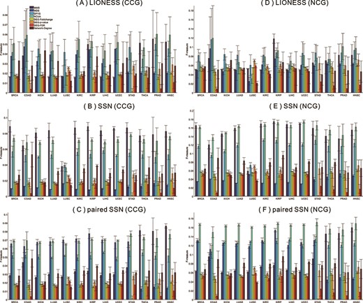
Performance comparisons of the network structure-based control methods (i.e. NMS, MDS, DFVS and NCUA) and the traditional methods (i.e. DEG–Foldchange, DEG–P-value, DEG–FDR and Network-Degree) on the different personalized state transition networks constructed by respectively using LIONESS, SSN and Paired-SSN methods. The personalized driver cancer genes from 13 cancer datasets are annotated in the lists of CCG, NCG and CSD databases. (A–C) are the results of the network structure-based control methods and the traditional methods in CCG list by respectively using the LIONESS, SSN and Paired-SSN network constructing methods; (D–F) are the results of the network structure-based control methods and the traditional methods in NCG list by respectively using the LIONESS, SSN and Paired-SSN network constructing methods.
(i) The network control methods are more effective for discovering the PDGs than the traditional DEG and Hub-gene selection method (Network-Degree). For example, in Figures 5 and 6, the F-measures of the network control methods are all higher than those of traditional methods, according to the enrichment of predicted personalized driver genes in the gold-standard cancer gene lists like CCG, NCG and CSD.
(ii) For the CCG and NCG lists, the F-measures of network control methods are dependent on the constructed personalized state transition networks, and we suggest SSN and Paired-SSN method as the preferred sample network construction method. For example, in Figure 5, we can see that for the CCG and NCG lists, the F-measures of network control methods would be higher when SSN and Paired-SSN networks rather than LIONESS are used.

Performance comparisons of the network structure-based control methods (i.e. NMS, MDS, DFVS and NCUA) and the traditional methods (i.e. DEG–Foldchange, DEG–P-value, DEG–FDR and Network-Degree) in the CSD list on the different personalized state transition networks which are constructed by respectively using (A) LIONESS, (B) SSN and (C) Paired-SSN methods.
(iii) For the CSD lists, the F-measures of network control methods show strong cancer sample heterogeneity in different cancer datasets. For example in Figure 6B and C, we can see that the F-measures of NCUA on SSN and Paired-SSN networks for BRCA cancer dataset are above 0.1, while the F-measures for lung squamous cell carcinoma (LUSC), kidney renal clear cell carcinoma (KIRC), kidney renal papillary cell carcinoma (KIRP) and uterine corpus endometrial carcinoma (UCEC) cancer datasets are much lower than 0.05. Such sample heterogeneity can also be observed by other network control methods, although they would detect different cancer sites or samples.
Summary of how to choose the network construction methods and network control methods for 13 kinds of cancer patients
| CCG | NCG | CSD | |
|---|---|---|---|
| BRCA | SSN_MMS | Paired-SSN_NCUA | Paired-SSN_NCUA |
| COAD | Paired-SSN_NCUA | Paired-SSN_NCUA | SSN_MMS |
| KICH | SSN_MMS | Paired-SSN_NCUA | SSN_MMS |
| LUAD | SSN_MMS | Paired-SSN_NCUA | SSN_MMS |
| LUSC | Paired-SSN_MDS | Paired-SSN_NCUA | Paired-SSN_DFVS |
| KIRC | SSN_MMS | SSN_MMS | LIONESS_MDS |
| KIRP | SSN_MMS | SSN_MMS | SSN_DFVS |
| LIHC | SSN_MMS | SSN_MMS | SSN_MMS |
| UCEC | SSN_MMS | SSN_NCUA | LIONESS_MDS |
| STAD | SSN_MMS | Paired-SSN_NCUA | SSN_MMS |
| THCA | Paired-SSN_MMS | Paired-SSN_NCUA | SSN_MMS |
| PRAD | Paired-SSN_MMS | Paired-SSN_NCUA | Paired-SSN_MMS |
| HNSC | Paired-SSN_MMS | Paired-SSN_NCUA | Paired-SSN_MMS |
By summarizing the comparison results of methods and datasets from Figures 5 and 6, we gave Table 5 to show how to choose the network construction method and network control method for 13 kinds of cancer patients according to the gene lists of CCG, NCG and CSD. In addition, the case of patient ‘TCGA-BJ-A28W’ in THCA cancer is used to show the performance of the network control approaches of MMS, MDS, DFVS and NCUA by choosing a sub-network of the personalized state transition network which contains FGR gene and its neighborhood genes. The results are shown in Figure 7. In this case, the genes of {BTK, ABL1, EPHA7} in CCG and NCG gene lists are considered as the gold standard driver genes. For MMS method, it identifies 10 genes of {EPHA7, DOK1, EPHA5, EGF, EFNB1, BLNK, CCL11, EDN1, FGR, EFNA1} as the driver genes of ‘TCGA-BJ-A28W’ patient, and there is one gold standard driver gene (EPHA7) among 10 driver genes. For MDS method, there are no gold standard driver genes among the identified driver genes. For DFVS method, it identifies the FVS node of DOK1 that intersects two feedback loops in the network as driver genes, and there are no gold standard driver genes among the identified driver genes. For the NCUA method, it identifies four driver genes of {FGR, ABL1, EDN1, CSK} which can cover all the edges (feedback loop) in the undirected network, and there is one gold standard driver gene (‘ABL1’) among these four driver genes.
To further support the efficiency of network control methods by statistical significance, the enrichment P-values (calculated by using the hyper geometric test [129]) of the predicted driver genes in CCG and NCG and CSD lists were evaluated for different network control methods as shown in Figures 8 and 9.
(i) From the results in Figure 8, we can see that network control methods are actually significant for predicting the PDGs enriched in the CCG and NCG lists.
(ii) Furthermore, from Figure 9, we found the following facts: for the CSD list, the enrichment P-values of network control methods vary in the different cancer datasets. For example for UCEC cancer dataset, all the network control methods (i.e. MMS, MDS, DFVS and NCUA) on SSN, Paired-SSN and LIONESS networks do not have significant enrichment results (Figure 9). But for other cancer datasets, there are significant P-value enriched in the CSD list by using the NCUA method on the Paired-SSN networks (Figure 9C).
(iii) For the CSD list, the enrichment P-value results of network control methods are dependent on the constructed personalized state transition networks, and we suggest the Paired-SSN method as the preferred sample network construction method. For example in THCA cancer dataset, MMS and DFVS and NCUA methods on the Paired-SSN networks are significantly enriched in CSD list (Figure 9C), while all the network control methods on the LIONESS networks are not significant (Figure 9A). Furthermore, for LUSC cancer dataset, the results of DFVS and NCUA on Paired-SSN network are significantly enriched in the CSD list (Figure 9C), while the P-values of all the network control methods on SSN and LIONESS networks are not significant for predicting the PDGs enriched in the CSD list (Figure 9A and B).
The paired samples of the 13 cancer datasets and gene annotation datasets (CCG, NCG and CSD gene lists) used in this work, and the evaluation pipeline called Cancer_Network_control package, can be freely downloaded at https://github.com/NWPU-903PR/Cancer_Network_Control. Especially, the evaluation pipeline can implement three kinds of the single-sample network construction methods (i.e. LIONESS, SSN and Paired-SSN) and four kinds of the network control methods (i.e. MMS, MDS, DFVS and NCUA) for detecting PDGs in cancer.
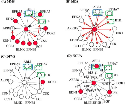
Schematic demonstration of MMS, MDS, DFVS and NCUA methods on the personalized state transition network constructed with the Paired-SSN method for patient ‘TCGA-BJ-A28W’ in THCA cancer. A sub-network (containing FGR gene and its neighborhood genes) of the personalized state transition network for the ‘TCGA-BJ-A28W’ cancer patient is chosen to evaluate the performance of MMS, MDS, DFVS and NCUA. The genes {BTK, ABL1, EPHA7} in the CCG gene list (within the rectangular box in blue color) and NCG gene list (within the rectangular box in green color) are considered as the gold standard driver genes. (A) MMS method found the matching edges (red color edges) which results 10 unmatched nodes (red color nodes). These 10 genes are considered as the driver genes in which there is one standard driver gene (EPHA7). (B) MDS method identified the MDS {FGR} (red color node) as driver genes in which there are no standard driver genes. MDS assumes that the driver node can independently control its associated edges (red color edges). (C) DFVS method identified the FVS node {DOK1} (red color node) that intersects two feedback loops as the driver genes in which there are no standard driver genes.(D) NCUA method identified four driver genes (red color nodes) which can cover all the edges (feedback loop) in the undirected network. There is one standard driver gene among four driver genes.
![The enrichment significance scores of the PDGs identified with the network structure-based control methods. The enrichment significant P-value is calculated by using the hyper geometric test [129]. The enrichment score ESg is defined as ESg = −log10(P-value). The personalized driver cancer genes from 13 cancer datasets are annotated in the lists of CCG, NCG and CSD databases. (A–C) are the results of the MMS, MDS, DFVS and NCUA methods in the CCG list by respectively using the LIONESS, SSN and Paired-SSN network constructing methods; (D–F) are the results of the MMS, MDS, DFVS and NCUA methods in the NCG list by respectively using the LIONESS, SSN and Paired-SSN network constructing methods; the red line denotes the significant threshold value ESG = 2. If the ESG for the predicted PDGs is larger than this threshold value, we think that the enrichment result is significant.](https://oup.silverchair-cdn.com/oup/backfile/Content_public/Journal/bib/21/5/10.1093_bib_bbz089/7/m_bbz089f8.jpeg?Expires=1750181400&Signature=XxlTTDPI-d~-wDpxScJuQ1sfYsfBtbQ6ObqeP9lOEnzeT9bN55bLz1eFiccmTY8Rf2Mlvyx4y8FbuEY3czNien6x0O2NRsUg0F5aIglYbQ8eXsg7vI8kKFWcKvYEO3SpM0bylHGQfzTOsNHN9K~zb20McEaEB5I0Av9e476MAn9rBTJv1y4uu8ppYKJkUPLbDwgFbqAKqiMci88CytHsULJ0JPPIHUtSqGvH~LPVBudHmiju3EdMPxJmqejNf4tDGU5ORshdeDtqrNhVp15MqXqUB-ACg0orhlgcoc8V7ur7HCQgtt2FzI7cNC2BSaATRpBIsCxTWitisXfF39Irig__&Key-Pair-Id=APKAIE5G5CRDK6RD3PGA)
The enrichment significance scores of the PDGs identified with the network structure-based control methods. The enrichment significant P-value is calculated by using the hyper geometric test [129]. The enrichment score ESg is defined as ESg = −log10(P-value). The personalized driver cancer genes from 13 cancer datasets are annotated in the lists of CCG, NCG and CSD databases. (A–C) are the results of the MMS, MDS, DFVS and NCUA methods in the CCG list by respectively using the LIONESS, SSN and Paired-SSN network constructing methods; (D–F) are the results of the MMS, MDS, DFVS and NCUA methods in the NCG list by respectively using the LIONESS, SSN and Paired-SSN network constructing methods; the red line denotes the significant threshold value ESG = 2. If the ESG for the predicted PDGs is larger than this threshold value, we think that the enrichment result is significant.
![The enrichment significance scores of MMS, MDS, DFVS and NCUA methods in the CSD list by respectively using the (A) LIONESS, (B) SSN and (C) Paired-SSN network constructing methods. The enrichment significant P-value is calculated by using the hyper geometric test [129]. The enrichment score ESg is defined as ESg = −log10(P-value). The red line denotes the significant threshold value ESG = 2. If the ESG for the predicted PDGs is larger than this threshold value, we think that the enrichment result is significant.](https://oup.silverchair-cdn.com/oup/backfile/Content_public/Journal/bib/21/5/10.1093_bib_bbz089/7/m_bbz089f9.jpeg?Expires=1750181400&Signature=PviG5ljzmg8mOqmIMgM8ZNxQmtCY5fkLigsLSm0v4J61LqzLrwZhM0daffxcE54139KjIHg7rfWi1nUZ2Apk5Ohmss~GG1XfE09Spp85TkrDQIECUYl2BgRpma~p6u~W8CdYgb8QU345ZV6M0EKt7wkyGV2sy0AM1-BKrGVTlh47R3P4ZkzlvK7e7ox4zF4CFB032C3Ed2al5~oLKgZ3gfWPWoNoDJtdh-2376fzh9F5YXc8AjkfAH46XxjyMpd4P2m9tCh7q80jnPpjDc9z4Hdevf4hYmbujoIV3kYG5josKAw1QW2HVcjU8gqPAOG1~fzR6fiwOZjev8Z9cw5kLw__&Key-Pair-Id=APKAIE5G5CRDK6RD3PGA)
The enrichment significance scores of MMS, MDS, DFVS and NCUA methods in the CSD list by respectively using the (A) LIONESS, (B) SSN and (C) Paired-SSN network constructing methods. The enrichment significant P-value is calculated by using the hyper geometric test [129]. The enrichment score ESg is defined as ESg = −log10(P-value). The red line denotes the significant threshold value ESG = 2. If the ESG for the predicted PDGs is larger than this threshold value, we think that the enrichment result is significant.
Remarks on the structure control methods
Many studies have focused on controlling the system through any minimum driver-node set, but little work has been conducted for multiple driver-node sets to control the network. From the perspective of identifying PDGs, the existing structural controllability may not be efficient or optimal, and this limitation hinders the application of network control methods in the fields of biology and biomedicine. With the recent rapid development of structural controllability, many applications to complex biological networks have verified that structural controllability can provide meaningful results. Liu et al. [101] defined the classification of nodes as being critical, redundant or ordinary if the node’s absence increases, decreases or is equal to the driver nodes, respectively. This classification has been applied to the identification of disease genes and drug targets in a directed protein interaction network [130]. The control capacity is introduced as a full controllability measure to quantify the importance of a node in networks [131]. Furthermore, the control capacity can be applied to the detection of driver metabolites in the human liver metabolic network [132], driver proteins in a human signaling network [133] and critical regulatory genes in a cancer signaling network [134]. Similarly, Guo et al. [23] applied control capacity in constrained target controllability to evaluate the controlling role of a single gene to detect driver genes in gene interaction networks. In addition, Bao et al. [135] presented an algorithm to compute and evaluate the critical, intermittent and redundant vertices for controlling direct networks under the Feedback control framework. Furthermore, physical controllability [136, 137] is an important metric to evaluate how much energy is required to achieve a control purpose for the structure-based control methods.
where B denotes the control matrix encoding the relationship between TF and genes. In this DGC method, it is assumed that the TF is a constant controller that produces constant quality signal (greater than zero) to change the network state from the initial state to the desired state in cell reprogramming. The control matrix B should be determined according to prior information, unlike the previously mentioned structure-based control methods. This DGC method provides a new perspective for investigating the controllability of networks from data and can be applied successfully to identify TF in cellular reprogramming. The DGC method, however, ignores the prior gene interaction data and also suffers from higher computational cost. Therefore, it is highly required that we will be able to identify PDGs in complex diseases with more accuracy and efficiency in the future.
Future directions
Human genomics is an area rightly shifting toward integrative analysis, in which accurately and reliably identifying PDGs is a key focus. Mathematical and computational modeling techniques are critical tools that enable us to design more personalized therapy schemes, as they allow for the analysis of large datasets and complex dynamic processes [57, 65]. This review introduced state-of-the-art techniques to enhance the connections between network control theory and the PDGs identification related to the biological system transition from the normal state to the disease state. These insights may provide novel clues for identifying individual disease genes for precision medicine. However, advances in molecular biology such as single-cell RNA sequencing (i.e. scRNA-seq) techniques can make it possible for developing more efficient methods to improve the PDGs discovery. This section will discuss future directions for the application of these controllability principles to benefit the PDGs identification.
Characterizing controllability of ncRNA regulatory network
As well known to us, cancer drivers can be divided into two types: coding drivers (genes) and non-coding drivers (e.g. miRNA, lncRNA). In this review, we mainly discuss the identification of personalized coding driver genes by using network control principles. However, computational identification of non-coding drivers is in many ways even more challenging than coding drivers owing to their complex and varied modes of action as well as our poor understanding of non-coding regions in general. The non-coding regions contain a wealth of regulatory sequences and non-coding RNAs (ncRNAs) whose role in cancer remains largely unknown [139]. No network control studies have investigated roles of ncRNAs in cancer, in particular at an individual level; we expect that future studies will discover novel candidate individual-specific ncRNAs drivers by using network control principles on the ncRNAs datasets [140]. Furthermore, it was reported that ncRNAs are highly expressed in a subset of cells in a population, while their expression tends to be lower than protein-coding mRNAs [141, 142]. Therefore, reconstructing the personalized state transition networks and designing the corresponding structure-based network control methods at the single cell level may efficiently identify non-coding drivers that are important in cancer.
Characterizing controllability of biological networks in single cells
The change of gene expression networks is dependent on a number of factors, including cell types and genetic signatures. The influence of each of these expressions can be determined by scRNA-seq data [84, 143]. Therefore, state transition networks found from bulk-based expression data cannot truly represent those found at the single-cell level, and single-cell transcriptome measurements can reveal unexplored biological diversity [144, 145]. Furthermore, scRNA-seq techniques allow researchers to quantify gene expression in up to thousands of individual cells [146]. For example to depict the baseline landscape of the composition, lineage and functional states of tumor infiltrating lymphocytes, Zhang et al. obtained 12 346 T cells scRNA-seq data from 14 treatment-naïve non-small-cell lung cancer patients [147]. Meanwhile they obtained transcriptomes of 11 138 single T cells from 12 patients with colorectal cancer and developed single T cell analysis by RNA sequencing and TCR tracking indices to quantitatively analyze the dynamic relationships among 20 identified T cell subsets with distinct functions and clonalities [148]. However, these scRNA-seq technologies suffer from many sources of technical noise and bias that must be modeled to account for the resulting uncertainty in downstream analyses, including undersampling of mRNA molecules (often called ‘dropout’), which can severely obscure important gene–gene relationships [149, 150]. The unique features of scRNA-seq data may provide opportunities to enhance personalized state transition networks, which will require the development of new algorithms to take these data features into account when constructing state transition networks to further improve PDGs identification at a single-cell level [151, 152].
Characterizing controllability of biological networks in edge dynamics
All of the above described works mainly focus on the identification of PDGs by exploiting dynamic analysis of node-networks. Recently, edge-network dynamic analysis has become a hot topic in both the edge (gene pairs) state network construction of single samples [97] and control principles of edge dynamic [51, 153–156]. Furthermore, recent studies have highlighted the importance of targeting key gene interactions for designing drug combinations in disease control [75, 157–159]. Therefore, how to identify the PDGs with proper network control methods by considering the edge dynamic of individual state transition network is an important direction in the future.
Characterizing controllability of biological network in temporal dynamics
The above-introduced techniques construct personalized state transition networks mainly by using personalized normal and tumor expression data; however, these methods ignore the personalized temporal data information. The usage of temporal expression data is important for identifying PDGs because it can provide additional dynamic information for inferring developmental trajectories of PDGs in cancer propagation [160]. Meanwhile, it remains a significant challenge to use temporal expression data to identify PDGs. The first issue is to obtain the personalized temporal data in complex diseases. Although modern sequencing technology has provided significant resource data to study human diseases, we still lack temporal data for a single patient. The second issue is to construct the personalized state transition networks and to further develop control models to identify PDGs by using such temporal expression data. Recently, some techniques on temporal data may provide new clues for identifying the PDGs with temporal data information, including detection for disease tipping points [161–162], dynamic network biomarker (DNB) discovery [163–164], DGC method [138], structural controllability of temporal networks [165–168] and personalized DNB identification [169].
Characterizing optional decision of network controllers
The existing research has focused mainly on the control roles of a single node and has ignored the control roles of different driver-node sets. When one actually expects to control a system for optimization, different driver-node sets may not participate equally in control and different sets of driver nodes may be related preferentially to specific biological function and progress [170]. To measure such control roles of different sets of driver nodes demands the ability to combine controllability and other control measures, such as time cost and energy cost, to obtain the optimal driver node set. Notably, the energy cost is a typical measure used to analyze the control objective, which is related with the usage of the controllers.
The existing structure-based control methods do not consider how to obtain the actual control by designing optimal controller or driver signal. Although feedback and closed-loop controllers have been applied to many physical systems [67, 171, 172], the task of designing a controller for structure-based control methods in biological networks remains unresolved. The constant controllers have been applied to identify the key TFs in cell reprogramming [138]. Therefore, we expect that such discussed controllers also will be able to enhance the key choice of different sets of driver nodes and to identify PDGs in personalized medicine or in the study of general biological transitions.
Identification of the personalized driver pathways by using network control principles
It is well known that different gene mutations may target the same pathway [173]. Therefore, it is necessary to shift the study from gene to pathway level, which is helpful in capturing the heterogeneous functional patterns in cancer. There have been several studies to discover the mutation patterns at the pathway level [174–176]. Different cancer types may have different network control principles at the pathway level, which is critical for personalized therapy (e.g. precision medicine in cancer treatment). Furthermore, several studies suggest that there are functional differences between different cancer types, even different samples with the same cancer [177]. Taking into account such cancer heterogeneity, it is indispensable to develop new algorithms from network control perspectives to discover personalized driver pathways.
Conclusions
Cancer can be perceived as a dysfunction in molecular networks that regulate molecular communications and cellular processes. Molecular networks, such as gene regulation networks or signaling networks, are highly adaptable and dynamic. Thus, to fully understand the mechanism of cancer progression, we need to understand the dynamics of these networks in accordance with control theory. Tumor heterogeneity differs in survival fitness, invasive potential and adaptability to the tumor microenvironment, which has been a primary obstacle for understanding the functional importance in personalized therapies. The ability to identify PDGs of individual patients can provide an efficient source of the PDGs and drug targets and is essential for understanding tumor heterogeneity. Most of the existing computational methods for analyzing driver genes, however, have mainly focused on the cohort information rather than the individual PDGs. Recently, structure-based network control approaches have given us the ability to investigate the controllability of the complex networks with an adequate knowledge of the network structure through a minimum set of the driver nodes. These structure-based network control approaches can make it possible to deeply understand the mechanism of PDGs in cancer progression.
In this review, we considered cancer progression of individual patients from a normal state to a disease state as a network control problem and gave a comprehensive review of the recent work including the network reconstruction methods on single samples and network control models to solve such problem. In addition, we gave a performance assessment of structure-based control methods on multiple cancer datasets from TCGA. We found that to identify the PDGs, network control methods are more effective than the traditional DEG methods, which are remarkably dependent on the single-sample network construction methods. However, there are still promising and on-going efforts for the accurate PDGs identifications with network control approaches, such as the usage of personalized data (e.g. single cells), identification of personalized non-coding drivers and personalized driver pathways.
Considering cancer progression from a normal state to a disease state as a network control problem to identify PDGs
Introducing several network construction techniques on single samples to bridge network control theory and PDGs identification
Providing a comprehensive review of the network control methods and assessing the performance of the network control methods for identifying PDGs
Providing evaluation data and pipeline for users to easily apply network control methods on PDGs identifications
Acknowledgements
We thank the reviewers for giving us valuable comments, which benefit for the improvement of this paper. We thank LetPub (www.letpub.com) for its linguistic assistance during the preparation of this manuscript. We thank the members of Tatsuya Akutsu’s laboratory in Bioinformatics Center, Institute for Chemical Research, Kyoto University for valuable discussions on this topic. We apologize that we cannot cite all related studies owing to the limited space of manuscript space.
Funding
This paper was supported by the National Natural Science Foundation of China (grant nos. 61873202, 61473232, 91430111, 31771476, 81471047, 11871456), National Key R&D Program (grant nos. 2017YFA0505500, 2016YFC0903400), Strategic Priority Research Program of the Chinese Academy of Sciences (grant no. XDB13040700), Natural Science Foundation of Shanghai (grant no. 17ZR1446100) and Shanghai Municipal Science and Technology Major Project (grant no. 2017SHZDZX01).
Wei-Feng Guo is currently working toward a PhD degree at the School of Automation from Northwestern Polytechnical University, China. His work is currently co-supervised by Professor Shao-Wu Zhang and Professor Luonan Chen. He does researches in design of complex network control algorithms and its applications to human cancer genomics.
Shao-Wu Zhang received a PhD degree at the School of Automation from Northwestern Polytechnical University, China, at 2004. He has been a professor in Key Laboratory of Information Fusion Technology of Ministry of Education, School of Automation, Northwestern Polytechnical University, China. His current research interests include bioinformatics, complex networks and machine learning.
Tao Zeng received BS, MS and PhD degrees from Wuhan University, Wuhan, China, in 2003, 2006 and 2010, respectively. Since 2013, he has been an associate professor in Key Laboratory of Systems Biology, Shanghai Institutes for Biological Sciences, Chinese Academy of Sciences and now in Shanghai Research Center for Brain Science and Brain-Inspired Intelligence, Shanghai, China. His research interests include bioinformatics, network biology, computational biology, machine learning and graph theory.
Tatsuya Akutsu received BE and ME degrees in aeronautics and a DE degree in information engineering from The University of Tokyo, Tokyo, Japan, in 1984, 1986, and 1989, respectively. He has been a professor with the Bioinformatics Center, Institute for Chemical Research, Kyoto University, Kyoto, Japan, since 2001. His current research interests include bioinformatics and discrete algorithms.
Luonan Chen received a BS degree from Huazhong University of Science and Technology, Wuhan, China, in 1984, and MS and PhD degrees from Tohoku University, Sendai, Japan, in 1988 and 1991, respectively. Since 2010, he has been a professor and the executive director at Key Laboratory of Systems Biology, Center for Excellence in Animal Evolution and Genetics, Center for Excellence in Molecular Cell Science, Institute of Biochemistry and Cell Biology, Shanghai Institutes for Biological Sciences, Chinese Academy of Sciences. His fields of interest are computational systems biology, bioinformatics and nonlinear dynamics. In recent years, he published over 300 journal papers and 2 monographs in the area of computational systems biology.
