


Abstract
Single-cell RNAsequencing (scRNA-seq) technologies have enabled the large-scale whole-transcriptome profiling of each individual single cell in a cell population. A core analysis of the scRNA-seq transcriptome profiles is to cluster the single cells to reveal cell subtypes and infer cell lineages based on the relations among the cells. This article reviews the machine learning and statistical methods for clustering scRNA-seq transcriptomes developed in the past few years. The review focuses on how conventional clustering techniques such as hierarchical clustering, graph-based clustering, mixture models, |$k$|-means, ensemble learning, neural networks and density-based clustering are modified or customized to tackle the unique challenges in scRNA-seq data analysis, such as the dropout of low-expression genes, low and uneven read coverage of transcripts, highly variable total mRNAs from single cells and ambiguous cell markers in the presence of technical biases and irrelevant confounding biological variations. We review how cell-specific normalization, the imputation of dropouts and dimension reduction methods can be applied with new statistical or optimization strategies to improve the clustering of single cells. We will also introduce those more advanced approaches to cluster scRNA-seq transcriptomes in time series data and multiple cell populations and to detect rare cell types. Several software packages developed to support the cluster analysis of scRNA-seq data are also reviewed and experimentally compared to evaluate their performance and efficiency. Finally, we conclude with useful observations and possible future directions in scRNA-seq data analytics.
All the source code and data are available at https://github.com/kuanglab/single-cell-review.
Introduction
Transcriptome profiling of cells can capture gene transcriptional activities to reveal cell identity and function. In conventional bulk gene expression analysis, a transcriptome is measured as an average of the transcription levels in a bulk population of cells collected from a biological sample and the bulk gene expressions are clustered to detect gene coexpression modules and sample clusters [1, 2]. Because bulk analyses ignore individual cell identities, they cannot investigate important biological problems at the single-cell resolution such as distinct functional roles of cells during early development, distinct cell types in complex tissues, cell lineage relationships and stochastic gene expression among cells. Single-cell RNA sequencing (scRNA-seq) has emerged and now widely used to quantify mRNA expression in individual cells [3, 4]. In scRNA-seq protocols, single cells are isolated with a capture method such as flow-activated cell sorting (FACS), Fluidigm C1 or microdroplet microfluidics and then the RNAs are captured, reverse transcribed and amplified for sequencing [4]. The applications of scRNA-seq have already led to important biological insights and discoveries, for example, understanding of tumor heterogeneity in cancer [5].
Clustering is also a necessary step to identify the cell subpopulation structure in scRNA-seq data, there are several unique challenges in the clustering analysis. First, technical noise and biases are introduced by cell-specific characteristics such as cell-cycle stages or cell size, as well as by technical/systematic sources such as capture inefficiency, amplification biases and sequencing depth. For example, the heavy polymerase chain reaction (PCR) amplification required by the tiny amount of RNA material in a single cell [6] also exponentially amplifies the biases. These biases and noise cause uneven coverage of the entire transcriptome and result in an abundance of zero-coverage regions and many ‘dropout’ genes [7, 8]. In addition, when multiple single-cell populations from a cohort of samples are analyzed together, the technical biases and biological variance across the populations dominate the clustering of the single cells, resulting in clustering by the sample of origin rather than by cells of similar types [9].
In this article, we review the recently developed statistical and machine learning methods for improving the clustering of scRNA-seq data. These new methods include (1) new data processing statistical methods for cell-specific normalization, the imputation of ‘dropouts’, projection and dimension reduction and cell marker identifications; (2) the conventional clustering methods modified or customized for scRNA-seq data, including partitioning-based clustering, hierarchical clustering, mixture models, graph-based clustering, density-based clustering, neural networks, ensemble clustering and affinity propagation; (3) new approaches to cluster scRNA-seq transcriptomes in time series data and multiple cell populations and to detect rare cell types. We also discuss several additional important computational aspects in scRNA-seq data clustering including similarity measures, feature representations and evaluations of the single-cell clustering results. In addition, we performed experiments comparing more than ten software packages to evaluate their clustering performance and efficiency on a large-scale scRNA-seq dataset. Finally, we conclude the review with discussions of several remaining computational challenges in single-cell clustering analysis.
Data preprocessing for clustering
In the clustering analysis of scRNA-seq data, data preprocessing is essential to reduce technical variations and noise such as capture inefficiency, amplification biases, GC content, difference in the total RNA content and sequence depth, in addition to dropouts in reverse transcription [8]. High-dimensional scRNA-seq data are typically normalized and projected to a lower-dimensional space by dimension reduction. Several computational methods have also been developed to address dropout events with imputation or better similarity measures.
Normalization
The raw scRNA-seq read libraries are usually normalized in two ways; cell normalization and gene normalization. Cell normalization is done to remove the amplification biases and other cell-specific effects inherent in the experimental protocols and can be achieved with commonly used read count normalization methods such as fragments per kilobase million, reads per kilobase million and transcripts per million (TPM), which normalizes each cell by the total number of short reads and a scaling factor. Unique molecular identifier (UMI)-based protocols, in principle, already avoid biases related to amplification and sequence depth since multiple reads associated with the same UMI are collapsed into a unique count [10]. However, since libraries are usually not sequenced in saturation (i.e. each uniquely tagged molecule is observed at least once), normalization has also been shown useful for this type of data [11–14]. Another alternative for cell normalization is to use spike-in sequences such as the external RNA control consortium molecules [15] based on the assumption that technical effects affect the intrinsic and extrinsic genes equally [10]. Note that it is also common to use log-transformed read counts after adding a pseudocount of 1 [9, 12, 16–19].
Gene normalization is also performed across samples to prevent the highly expressed genes from dominating the analysis. For example, |$z$|-score normalization (standardization) [9, 12, 17] can be used, as in principal component analysis (PCA). Empirically, standardization of the features may improve the convergence and clustering. It is important to note that the standardized data will lose the relative scale of the genes and become less sparse due to the expression shift, which might influence clustering performance on large-scale sparse scRNA-seq data.
The SINCERA pipeline [20] provides a normalization component for preprocess scRNA-seq data. The package performs gene normalization by |$z$|-score and cell normalization by trimmed mean. To determine if trimmed mean should be performed, SINCERA also provides a quality-control tool for visualizing MA plot, Q-Q plot, intersample correlation and distance measures.
Other methods perform more specialized normalization on scRNA-seq data. For example, BISCUIT [21] uses iterative normalization during clustering procedure by learning parameters that represent the technical variations. Rare cell type identification (RaceID) [22] normalizes the total transcript count within each cell to the median transcript number across cells. Transcript-compatibility counts (TCC)-based clustering [13] uses equivalence classes instead of genes as features and normalizes each feature by dividing the total count across all the cells.
Moreover, it is typical to remove genes and cells from the library if they exhibit extremely low expression because of the assumption that they represent spurious signals in the data. Previous studies established different thresholds for the removal of low-expressed genes and cells, which might vary according to the total number of cells and genes in the analysis. For instance, in the analysis of droplet-based peripheral blood mononuclear cell (PBMC) data in single-cell variance-driven multitask clustering (scVDMC) [9], genes that are expressed in less than three cells, and cells with a total UMI count of less than 200 are removed from the analysis.
Although the global normalization of genes and cells is common in most of the current clustering workflows, there is still some debate regarding the effect on the clustering results. The analysis in [10] shows that the application of bulk-based cell normalization methods can have serious adverse consequences for the analysis of scRNA-seq data such as detection of highly variable genes before clustering in the presence of high level of technical noise and dropouts. Similarly, the analysis in [21] shows that global normalization by median library size or through spike-ins would not resolve the dropouts and might remove biological stochasticity specific to each cell type, both of which result in improper clustering and characterization of the latent cell types.
Dropout imputation
A significant technical artifact in scRNA-seq data is known as ‘dropout’. Dropout events refer to the false quantification of a gene as unexpressed due to missing or low-expressed transcripts during the reverse-transcription step [3]. Previous studies also suggested that simple normalization will not address the dropout effects in scRNA-seq data analysis [10, 21]. Thus, several clustering algorithms include specific mechanisms for the correction of dropouts, e.g. Seurat [11] use coexpression patterns across cells in the scRNA-seq profiles to impute the expression of the landmark genes from the coexpressed genes before clustering.
Dropouts can also be imputed while computing the pairwise similarity or distance for clustering. Clustering through imputation and dimensionality reduction (CIDR) [16] imputes the expression of the dropout genes before clustering. First, the occurrence of possible dropouts among the single cells is analyzed to identify the dropout candidates in each cell and calculate the dropout rate of each gene. The dropout rates of the candidates are then used to estimate the imputed expression levels of the dropout candidates between each pair of samples, i.e. when a dropout event is identified with high probability, the algorithm performs a weighted imputation of the expression from the expression profile of the other sample. Finally, cell–cell dissimilarity is calculated using the imputed values for hierarchical clustering. The new version of Seurat [12] and shared nearest neighbors (SNN)-Cliq [18] are based on SNN as an alternative similarity measure. It has been demonstrated that in sparse high-dimensional data, SNN is more suitable for clustering analysis in the presence of dropouts because of taking into account the surrounding neighbor datapoints. Therefore, these methods are also expected to perform better even without explicit imputation of the dropouts.
Zero-inflated factor analysis (ZIFA) [23] implements a modified probabilistic PCA to incorporate a zero-inflated model to account for the dropout events. ZIFA projects single cells to a low-dimensional space in which dropouts can happen with a probability specified by an exponential decay associated with the expression levels. The zero-inflated negative binomial-based wanted variation extraction [24] uses zero-inflated binomial model to extract low-dimensional signals from the data to account for zero inflation (dropouts), overdispersion and the nature of the count data. ZIFA-WaVE models the cells’ expression density function as an affine combination of a Dirac function, which accounts for the existence of dropouts, and a negative binomial distribution over the observed counts. ZIFA-WaVE fits the UMI counts better than ZIFA does without assuming an exponential decay of the expression values.
In a more sophisticated probabilistic graphical model, BISCUIT [21] explicitly estimates the imputed gene expressions in each single cell as well as the parameters of the assumed data distributions and prior distributions to represent technical and biological variations. In particular, random variables representing the unobserved true expression levels without the cell-specific rescaling are introduced in the graphical model for inference by Gibbs sampling. Thus, BISCUIT imputes the dropouts along with clustering by a Dirichlet process mixture model (DPMM).
Dimension reduction
Dimension reduction is commonly used to project high-dimensional gene expression data to a lower-dimensional space to allow the analysis to focus on relevant signals in the low-dimensional space for better data visualization, clustering and other interpretations. Dimension reduction also helps partially resolve the statistical issues of insufficient samples when the number of dimensions is larger than the number of samples. Many dimension reduction methods have been applied with scRNA-seq clustering algorithms including PCA, multidimensional scaling (MDS), t-distributed stochastic neighbor embedding (t-SNE), canonical correlation analysis (CCA), latent Dirichlet allocation (LDA) and dimension reduction embedded in other models.
PCA projects the datapoints with the eigenvectors (principal components) associated with the largest eigenvalues of the covariance matrix to preserve most of the variance in the original data. For example, pcaReduce [25] projects an expression matrix with the top K-1 principal components before clustering. SC3 [26] applies PCA and Laplacian transformations to the distance matrices to obtain inputs for its consensus clustering. PCA has also been widely used for data visualization in 2 or 3 dimensions after scRNA-seq data clustering [14, 16, 17, 19, 25]. PCA is a linear projection method based on assuming the data are Gaussian. To capture nonlinear structure in the data, kernel PCA can be applied with nonlinear kernel mapping.
MDS [27], also known as principal coordinate analysis (PCoA), is a dimension reduction algorithm based on distance-preserving techniques. MDS projects the data points to a lower-dimensional space to preserve the distance among the data points in the original higher-dimensional space by minimizing the difference between the distance in the original space and the distance in the projected space in all pairs of datapoints. For example, CIDR [16] applies MDS on a dissimilarity matrix and then takes the top principal coordinates for hierarchical clustering. MDS has the advantage of preserving the original pairwise distance in the low-dimensional projection and easily allowing nonlinear feature embedding. However, MDS is not scalable to large-scale data since pairwise distances must be computed to minimize the objective function.
t-SNE [28] is a probabilistic distance-preserving approach. t-SNE constructs a probability distribution associated with the similarities among the datapoints in the original space and the lower-dimensional space after projection and then minimizes the Kullback–Leibler divergence between the two distributions with respect to the locations of the data points in the map. t-SNE is widely used for data visualization in single-cell data analysis [12–14, 17, 19, 21, 22, 29–31].
CCA [32] is a dimension reduction method based on the cross-covariance of datasets. Given two or more datasets, the method finds projections of each dataset to maximize the correlation among the projected datasets. In scRNA-seq data analysis, CCA is suitable for the integration of data from multiple sources. For example, Seurat 2.0 [12] applies CCA on multiple single-cell datasets to identify the shared components.
LDA [33] was originally proposed in natural language processing. LDA assumes that a document is generated by first sampling topics from a multinomial distribution over the topics with a Dirichlet prior, followed by sampling of the words in the documents from the multinomial distribution over the words conditioned on each topic with a Dirichlet prior. Each document can then be represented in a lower-dimensional space of |$k$| topics. cellTree [34] uses LDA to learn ‘topics’ as latent features to represent cells, where words are gene expression levels conditioned to the selected latent features. The generative process of LDA produces an interpretable set of latent features.
Self-organizing map (SOM) [35] or Kohonen neural network is an unsupervised competitive learning algorithm that can be used for both clustering and dimension reduction by the number and arrangement of the output units of the neural network [36, 37]. When used for visualization, SOM organizes the output units of the neural network in a 2D grid to allow direct visualization of the clusters of datapoints.
Model-embedded dimension reduction combines dimension reduction within the models for data processing. ZIFA [23] and ZINB-WaVE [24] are two such examples that model dropout events by zero-inflated data for dimension reduction, as discussed in Dropout imputation section.
Similarity and kernel functions
Instead of using dimension reduction, many clustering methods use a kernel function or a similarity function to compute pairwise similarity between individual cells for clustering. The kernel strategy will compute a |$N \times N$| similarity matrix from an |$N \times M$| expression profile matrix expecting that smart design of the kernel mapping or the similarity function will reduce the variability in the original feature space in an implicit feature mapping with the function (if a valid kernel function is used). SNN-Cliq [18] and Seurat [11] use the SNN as the similarity graph. cellTree [34] finds a pairwise distance between cells by chi-square on the topic histograms found with LDA. DTWscore [38] finds the dynamic time warping (DTW) distance between pairs of cells for each gene using time series scRNA-seq data to select highly variable genes where the DTW distance is calculated based on the alignment of two time series in the optimal warping path. TCC-based clustering [13] uses Jensen–Shannon distance between cells as input for spectral clustering or affinity propagation. SIMLR [39] combines multiple kernels to learn a cell similarity matrix and address dropout issues with a rank constraint and graph diffusion.
Most other methods use more standard correlation or distance functions. BackSPIN [29], DendroSplit [17], ICGS [40] and SINCERA [20] use a Pearson correlation matrix to find the best splitting point in their hierarchical clustering strategy. GiniClust [14] and RaceID [22] also use a correlation matrix for DBSCAN and |$k$|-means clustering, respectively. Reference component analysis (RCA) [19] calculates the correlation between the expression profiles between single cells and reference bulk cells as new features for clustering to minimize technical variation and batch effect. CIDR [16] uses pairwise Euclidean dissimilarity on the expression profiles with the imputation of dropouts. SC3 [26] calculate cell–cell pairwise similarity or distance using Spearman, Pearson and Euclidean distances as multiple scenarios for consensus clustering.
Clustering techniques
In this section we review the application of eight categories of clustering methods to scRNA-seq data. The methods are summarized with their strenghts, limitations and time complexity in Table 1. Some scRNA-seq clustering algorithms use multiple clustering techniques and are thus listed in multiple categories.
Clustering techniques. The table shows the main categories of clustering algorithms applied to clustering scRNA-seq data. For each category, we include a list of scRNA-seq data clustering algorithms with their strengths, limitations and time complexity.
| Category / Subcategory | Strengths | Limitations | Time complexity | Algorithm | Year | |
| Partition | k-Means | - Low time complexity -Scalable to large datasets | - Sensitive to outliers -User must know the number of clusters | |$O(KND)$| | pcaReduce [25] | 2016 |
| SAIC [30] | 2017 | |||||
| SC3 [26] | 2017 | |||||
| SCUBA [41] | 2014 | |||||
| scVDMC [9] | 2018 | |||||
| |$k$|-Medoids | -Centers are original datapoints (medoids) - Suitable for discrete data | - Sensitive to outliers -User must know the number of clusters | |$O(K(N-K)^2)$| | RaceID2 [42] | 2016 | |
| Hierarchical | - Allow fitting to flexible cluster shapes - Hierarchical relationship among datapoints | - High time complexity - No explicit clusters given | - Agglomerative: |$O(N^2\log (N))$| - Divisive: |$O(2^N)$| | BackSPIN [29] | 2015 | |
| cellTree [34] | 2016 | |||||
| CIDR [16] | 2017 | |||||
| DendroSplit [17] | 2018 | |||||
| ICGS [40] | 2016 | |||||
| RCA [19] | 2017 | |||||
| SC3 [26] | 2017 | |||||
| Graph-based | Spectral clustering | - No assumption about data distribution | -Computationally intensive for large datasets | |$O(N^3)$| | TCC [13] | 2016 |
| SIMLR [39] | 2017 | |||||
| Clique detection | - Intuitive and clear definition of clusters as cliques | - NP-hard - Reliant on heuristic solutions - No cluster detection in sparse graph | |$O(2^N)$| | SNN-Cliq [18] | 2015 | |
| Louvain | - Relatively low time complexity | - Heuristic can lead to bad results - Iterative process can hide small communities | |$O(N\log (N))$| | SCANPY [49] | 2018 | |
| Seurat 1.0 [11] | 2015 | |||||
| Mixture models | -Incorporating prior knowledge as assumptions of distributions | - Computational difficulties in inference of graphical models | |$O(N^2K)$| (GMM) | BISCUIT [21] | 2016 | |
| DTWScore [38] | 2017 | |||||
| Seurat 1.0 [11] | 2015 | |||||
| TSCAN [46] | 2016 | |||||
| Densitybased | DBSCAN | - High efficiency - Flexible definition of clusters in arbitrary shape | - Sensitive to parameters | |$O(N\log {N})$| | GiniClust [14] | 2016 |
| Density peak clustering | - Does not require threshold parameter | - High time complexity | |$O(N^2)$| | Monocle 2 [51] | 2017 | |
| Neural network | -Incorporation of relation among clusters - Scalable stochastic gradient decentfor training | - Sensitive to parameters | |$O(KND)$| | Lv, Dekang, et al. [55] | 2016 | |
| Kim, Daniel, et al. [53] | 2015 | |||||
| SCRAT [54] | 2017 | |||||
| SOMSC [56] | 2017 | |||||
| Ensemble | - Robust clustering by integration of multiple methods | - Reliant on combining other clustering algorithms for ensemble | - Complexity of each algorithm in the ensemble | conCluster [31] | 2018 | |
| SC3 [26] | 2017 | |||||
| Affinity propagation | - Automatic detection of the number of clusters | - Sensitive to outliers | |$O(N^2)$| | TCC [13] | 2016 | |
| SIMLR [39] | 2017 | |||||
Partitioning-based clustering
Partitioning-based clustering methods identify the best |$K$| centers to partition the datapoints into |$K$| clusters where the centers are either centroids (means), called |$k$|-means or medoids, called |$k$|-medoids.
The |$k$|-means approach finds the centroids to minimize the sum of the squares of the Euclidean distance between each datapoint and its closest centroid. It has the advantage of low time complexity. However, it is sensitive to outliers, and the user must specify the number of clusters |$K$| a priori. The time complexity of |$k$|-means using Lloyd’s algorithm is |$O(KND)$| per iteration for clustering |$N$| datapoints of dimension |$D$| into |$K$| classes.
Several methods for analyzing scRNA-seq data employ |$k$|-means. SAIC [30] combines |$k$|-means and ANOVA in iterations of clustering single cells followed by signature gene identification. SCUBA [41] uses |$k$|-means to divide cells at each time point into two groups and uses gap statistics to identify bifurcation events. One of the steps of SC3 [26] is to use |$k$|-means on the projections of cells pairwise distance matrices and combine the individual |$k$|-means clustering results with a consensus function. pcaReduce [25] and scVDMC [9] use |$k$|-means to initialize their algorithm.
The |$k$|-medoids approach identifies |$K$| data points among the original |$N$| examples as medoids to minimize the sum of distance of data points to their medoid. It is most suitable for discrete data with meaningful medoids as clustering centers. However, similar to |$K$|-means, it is sensitive to outliers, and the user must specify the number of clusters |$K$| a priori. The time complexity of |$K$|-medoid using the partitioning around medoids algorithm is |$O(K(N-K)^2)$| for solving the combinatorial problem of choosing the optimal |$K$| points from the |$N$| data points.
RaceID2 [42], proposed for the identification of rare cell types with scRNA-seq data, showed that replacing |$K$|-means clustering with |$K$|-medoids leads to improved clustering results.
Hierarchical clustering
Hierarchical clustering is the most widely used clustering method in gene expression data analysis. Hierarchical clustering builds a hierarchical structure among the data points, which naturally defines clusters by the branches in the hierarchical tree. Many scRNA-seq data clustering algorithms are based on hierarchical clustering or adopt hierarchical clustering as one of the steps in the analysis.
Hierarchical clustering makes few assumptions regarding the overall distribution of the data points. Thus, it is suitable for datasets of many different shapes. Another important advantage is the representation with hierarchical relationships among all the datapoints for interpretation of the results. There are two main implementations of hierarchical clustering: agglomerative clustering and divisive clustering.
Agglomerative clustering starts with all the |$N$| datapoints as |$N$| initial clusters, and at each step, the clusters are merged according to distance measures, called linkage distance, until all the clusters are merged together at the root of the hierarchical structure. Agglomerative clustering using the CURE algorithm [43], for example, has the time complexity of |$O(N^2\log {N})$|. Divisive clustering, in contrast, starts with all the datapoints as a single cluster, and at each step the clusters are recursively divided. Divisive clustering with exhaustive search has complexity |$O(2^N)$|. Thus, the time complexity of hierarchical clustering is high. Moreover, the hierarchical relationship does not provide the optimal partition of the data points into clusters. An additional step is needed to derive a target number |$K$| of clusters from the hierarchical tree.
BackSPIN [29] is a two-way biclustering algorithm that applies hierarchical clustering on both single-cell and gene dimensions. BackSPIN iteratively splits the gene expression correlation matrix with SPIN [44] until the split criteria are no longer met at a branch. cellTree [34] builds a hierarchical structure among the single cells by constructing a minimal spanning tree on the topic distributions obtained by modeling single-cell data as a mixture of topics with LDA. CIDR [16] uses hierarchical clustering on the top coordinates obtained with PCoA on a dissimilarity matrix obtained with imputation of dropouts. ICGS [40] applies hierarchical clustering to cluster the expression data of a set of guide genes selected by filtering genes by expression level and dynamic range and performs pairwise correlation analysis. RCA introduced in [19] applies hierarchical clustering on the correlation matrix obtained from the projections of each single-cell sample onto the bulk and the scRNA-seq profiles. SC3 [26] also applies hierarchical clustering on the consensus matrix obtained by combining results of each |$K$|-means clustering in the ensemble. To derive the actual clusters in the hierarchy, DendroSplit [17] detects clusters in the constructed tree with dynamic splits and merges of the tree branches by measuring a separation score from the original expression data.
Mixture models
Clustering by mixture models assumes that the datapoints are sampled from a mixture of several probability distributions, each of which represents a cluster. The clustering of a sample is inferred by learning the probability of its generation from each distribution. The common choices of mixture models for clustering are the Gaussian mixture model (GMM) for continuous data and the categorical mixture model for count data.
The advantage of mixture models include rigorous probabilistic modeling and the flexibility of introducing prior knowledge in the model. However, solving mixture models requires advanced optimization or sampling techniques with high computational complexity and relies on the accuracy of the assumption about the data distributions. Mixture models are usually learned with expectation maximization, which alternatively infers the mixture parameters and class assignment likelihoods or sampling and variational methods for learning graphical probabilistic models. The time complexity of mixture models depends on the distribution of the mixture. In GMM clustering, the time complexity is |$O(N^2K)$| [45].
BISCUIT [21] is based on a hierarchical Dirichlet process mixture model (HDMM) with additional cell-specific scaling and dropout imputation. The HDMM models cells as a Gaussian mixture with Dirichlet prior on mixture coefficients, normal prior on the means and Wishart prior on the covariance matrices, and the cell-specific scaling accounts for cell-specific technical variances. BISCUIT is inferred with Gibbs sampling. Seurat 1.0 [11] combines scRNA-seq data with in situ RNA patterns for spatial clustering of the single cells. The scRNA-seq data are integrated with binarized in situ RNA data in a bimodal mixture model for a set of selected landmark genes, and then each single cell can be assigned to the spatial cluster regions by the posterior probability of the scRNA-seq expression profile in the bimodal mixture models. DTWScore [38] selects highly divergent genes from time-series scRNA-seq gene expression data with a DTWscore and then applies GMM to cluster cells with the selected genes. TSCAN [46] clusters cells using GMM and builds a minimum spanning tree (MST) to discover pseudotime ordering.
Graph-based clustering
In graph-based clustering, datapoints are represented as nodes in a graph, and the edges are represented by the pairwise similarities between the datapoints. Graph-based clustering is based on the simple assumption of dense communities in the graph represented as either a dense subgraph or spectral components, and thus relies less on other assumptions about the data distributions. However, the computational requirement is a major limitation. The two most common algorithms for graph-based clustering are spectral clustering and clique detection.
In spectral clustering [47], an affinity matrix and its graph Laplacian are built by a similarity function, such as RBF kernel. The top eigenvectors of the graph Laplacian are computed for subsequent clustering by |$K$|-means. The time complexity of finding all the eigenvectors is |$O(N^3)$|, although more efficient methods can be used to find a certain number of top eigenvectors. Thus, spectral clustering is often not directly applicable to large datasets. TCC-based clustering [13] builds an affinity matrix with transcript compatibility counts using the Jensen–Shannon distance between cells for spectral clustering when the number of cell types is known a priori; otherwise affinity propagation is applied. SIMLR [39] is a framework for learning a cell similarity measure using rank constraint and graph diffusion, by which the learned latent components can be used for spectral clustering.
In graph theory, a clique is defined as a subgraph in which every pair of nodes are adjacent. The cliques, therefore, represent clusters of datapoints in the graph. Since finding cliques in a graph is an NP-hard problem, heuristic approaches are often used. SNN-Cliq [18] utilizes clique detection to cluster cells with scRNA-seq data. Since cliques are often rare in sparse graphs, SNN-Cliq detects dense but not fully connected quasi-cliques in an SNN graph.
Another graph-based clustering algorithm for single-cell analysis is the Louvain algorithm [48]. Louvain is a community detection algorithm that is more scalable than other graph-based algorithms using a greedy approach to assign nodes to communities and updating the network to obtain more coarse-grained representation. The time complexity of Louvain is |$O(N \log {N})$|. SCANPY [49] is a pipeline that integrates the Louvain algorithm to provide a tool capable of analyzing a large scale scRNA-seq datasets. Seurat [11] also utilizes the Louvain algorithm on the SNN graph of cells to discover cell types.
Density-based clustering
Density-based clustering defines clusters as regions with a high density of datapoints in the input space. Two examples of density-based clustering are DBSCAN and density peak clustering.
DBSCAN [50] reports a cluster if, for a given datapoint taken as the center of a sphere of radius |$\epsilon $|, the number of datapoints inside the sphere is larger than a threshold. The process is repeated for each datapoint to expand the cluster. It has the advantages of high efficiency and suitability for data with any shape. However, clustering by density is very sensitive to the parameters and can exhibit poor results if the densities of the clusters are unbalanced. The time complexity of the DBSCAN clustering is |$O(N\log {N})$|. Density-based clustering is typically used for identification of outlier cells in scRNA-seq data analysis, such as GiniClust [14] and Monocle 2 [51].
GiniClust [14] is based on DBSCAN to discover rare subpopulations of cells. GiniClust uses the Gini index as a measure of the variability of expression values to select the genes that are then used by DBSCAN to cluster cells.
Density peak clustering [52] takes into account the distance between datapoints instead of a density threshold as in DBSCAN and assumes that cluster centers are local maxima in the density of datapoints in the cluster. The time complexity of density peak clustering is |$O(N^2)$|. Monocle 2 [51] performs density peak clustering [52] on cells in the space obtained by t-SNE.
Neural networks
The Kohonen neural networks, also known as SOMs [35] performs competitive learning for clustering; each training datapoint is used iteratively to update the cluster centers weighted by the similarity (distance) between the training datapoint and each center with stochastic gradient-descent. The cluster centers are initialized with predefined structures, such as a grid. SOM is quite scalable since stochastic gradient-descent does not require keeping all the datapoints in memory. In addition, the predefined structures among the centers can introduce prior knowledge and provide interpretable relationships among the clusters. SOM is, however, sensitive to parameter tuning, such as the learning rate used to update the weights. It can be solved with a similar algorithm to that of |$K$|-means in |$O(NKD)$|.
SOM has been used for visualizing and clustering scRNA-Seq data. Several studies [53–55] applied SOM to intuitively visualize similarity relationships in a 2D heat map in which the spatial proximity reflects the expression pattern similarity. The software package single-cell R-analysis tools (SCRAT) [54] provides users with options to visualize a 2D heat map representing correlations among genes across single-cell profiles. SOMSC [56] utilizes SOM to collapse high-dimensional gene expression data into two dimensions for cellular state transition identification and pseudotemporal ordering of cells.
Ensemble clustering
Ensemble clustering, also called consensus clustering, is a widely used strategy in which clustering is performed using several different scenarios (e.g. different clustering algorithms, similarity measures and feature selections/projections) with the same dataset, and the individual results are later merged based on the agreement among them by a consensus function. Ensemble learning can capture the diversity in different data representations and clustering models and has been shown to be more robust and lead to better results than single models. The limitation of ensemble clustering is the reliance on other techniques for data transformation and the base clustering methods.
SC3 [26] is a consensus clustering method applied to scRNA-seq data clustering. SC3 first finds cell pairwise distance matrices by Euclidean, Pearson and Spearman distance followed by PCA and Laplacian transformations. Then, six different kinds of projections are clustered by |$K$|-means to allow the construction of a consensus matrix with CSPA consensus function [26]. Finally, the consensus matrix is used for hierarchical clustering. conCluster [31] is another consensus clustering method that combines several partitions by t-SNE and |$K$|-means with different parameters. The partitions are then concatenated as the consensus for final |$K$|-means clustering.
Affinity propagation
Affinity propagation [57] is a clustering algorithm based on message passing between two kinds of log-probabilities to find exemplar datapoints (cluster centers): responsibility, which indicates how suitable a datapoint |$x_k$| is to represent a datapoint |$x_i$| relative to other candidates |$x_{k^{\prime}} \neq x_k$|, and availability, which measures how appropriate datapoint |$x_i$| is for representation by datapoint |$x_k$|, considering other datapoints |$x_{i^{\prime}} \neq x_i$| also represented by |$x_k$|. The main advantage of affinity propagation is that there is no requirement that the number of clusters be known. The disadvantages are the relatively high time complexity and the sensitivity to outliers. The time complexity of affinity propagation is |$O(N^2)$|. TCC-based clustering [13] clusters single cells with affinity propagation when the number of cell types is unknown. SIMLR [39] also has the option to apply affinity propagation directly on the similarity matrix learned from multiple kernels instead of spectral clustering on the latent space.
Clustering multiple cell populations
When multiple single-cell populations collected from multiple biological samples are sequenced, more complex batch effects and specific biological variations in each individual cell population are introduced into the clustering analysis. Batch effects occur when cells from one biological group or condition are cultured, captured and sequenced separately from cells in a second condition [58]. If each cell population is collected from one individual in a group of samples such as a patient cohort, each individual single-cell population will carry distinct population-specific characteristics. The technical biases and irrelevant biological variance among the samples will be significant confounding factors causing the individual cell populations to cluster together. For example, when the scRNA-seq profiles from multiple patients are pooled together for clustering, the clusters will simply assign the single cells to the sample origin [9].
where |$X^{(d)}$| represents the gene expression profile of population |$d$|; |$D$| is the number of populations; |$B \in \{0,1\}^m$| is an indicator vector of gene selection; |$D_B$| is a diagonal matrix with |$B$| on the diagonal and |$Y^{i,j} = [U_{i,j}^{(1)},\dots ,U_{i,j}^{(D)}]^T$|.
Seurat 2.0 [12] identifies cell subpopulations by integrating multiple data sets with a common source of variation with multiple CCA (multi-CCA) [59] to learn shared gene correlation structures conserved across the multiple datasets. Similar to the CCA discussed in Dimension reduction section, multi-CCA combines pairwise CCA to find the optimal coprojection of each dataset to maximize the total correlation between each pair of projections. The cells projected into the lower-dimensional space are then used to find cell–cell distance by SNN, and cell types are discovered by a graph-based clustering method, smart local moving [60].
These advanced data integration models explored important general frameworks for cross-dataset studies in single-cell data analysis that enable future studies from consortia to integration of datasets from multiple laboratories and technologies aiming to define, for example, all human cell types.
Rare cell types and singleton clusters
In single-cell clustering analysis, the detection of rare cell types is an important problem since cell types that play an important role in development or disease progression often have low abundance [14]. Due to their small population size, rare cell types are often difficult to detect in standard clustering analysis.
RaceID [22] is a clustering algorithm specifically designed to identify rare cell types in scRNA-seq data. The algorithm first computes Person’s correlation distance between pairs of cells used for |$K$|-means clustering. In each cluster, outlier cells are screened according to the variability of genes compared to a background noise model. Finally, the outlier cells are merged into outlier clusters if their correlation exceeds a threshold of the cell–cell correlation in their original cluster.
GiniClust [14] is another clustering strategy focused on the discovery of rare subpopulations. The algorithm uses the Gini index as a measure of the variability in expression values, for gene feature selection. This approach is shown to be more sensitive to the proportion of cells with high versus low expression values than the commonly used Fano factor. The genes with the highest Gini index are then used as features for density clustering by DBSCAN to detect the rare cell types.
Cells belonging to rare cell types can also be viewed as outliers in the clustering process. Most published single-cell clustering algorithms can result in small clusters, or even singletons. Although this may occur due to poor initialization or convergence of the clustering algorithm, it can also be interpreted as outlier cells from rare cell types. Several algorithms have specific techniques, and parameter tuning in most cases to carefully select these singletons for rare cell-type detection. SINCERA [20], for example, instead of requiring the user to specify the minimum distance between the clusters in hierarchical clustering, uses a threshold on the number of allowed singletons. Similarly, DendroSplit [17] has three parameters that control the number of detected singletons: minimum cluster size; disband size, which evaluates the size of subtrees resulting from a cluster split; and a threshold to determine singleton merging to its nearest neighbor.
Cell differentiation and pseudotime ordering
Cell differentiation is governed by complex gene-regulatory processes. During differentiation, each cell makes independent fate decisions by integrating signals from other cells and executing complex gene-regulatory changes. scRNA-seq data have been analyzed to reconstruct the lineage trees of the cell differentiation processes and to sort cells according to their biological stage, also called pseudotime. Although the details of the methods specifically designed for this problem are beyond the scope of this article, we noticed that several of the methods are also either applicable to single-cell clustering or based on some clustering strategies. These methods usually find some specific projections by dimension reduction for tree construction or clustering in low-dimensional space.
Monocle [61] utilizes independent component analysis to find a low-dimensional projection of the cells, which are then used to construct a MST. The more recently proposed Monocle 2 [51] reconstructs single-cell trajectories with reverse graph embedding, utilizing only genes differentially expressed in cell clusters identified by t-SNE and density peak clustering. TSCAN finds clusters using the GMM and builds an MST based on the clusters for pseudotime ordering. cellTree [34] applies the LDA to project the individual cells into the topics dimension to represent individual cells as a mixture of topics. The cell hierarchical structure can then be found by finding the MST on a chi-square distance matrix computed with topics histograms. SLICER [62] uses locally linear embedding to project the cells in a lower-dimensional space to build new neighbor graph for sorting the cells based on their shortest path distances from a user-specified starting cell. Then, a geodesic entropy is computed using the shortest path distances to detect branches in the cellular trajectory. SCUBA [41] uses |$K$|-means to cluster cells along a binary tree detailing bifurcation events for time-series data. SOMSC [56] utilizes SOM to reduce the dimension of gene expression data to identify cellular states, and the pseudotime ordering of the cells is obtained from the state transitions.
Discovery of cell marker genes
One of the most important goals in the clustering analysis of the scRNA-seq data is the discovery of new marker genes to characterize the gene expression patterns and functions of each cell type found by clustering for future biological interpretation and experimental validation. Most methods identify marker genes after clustering by differential gene expression analysis between the clusters with statistical tests. Seurat [11], for example, uses the Wilcoxon rank-sum test, a nonparametric test based on the order statistics in the sorted expression values. SINCERA [20] also uses the rank-sum test when the sample size is small and Welch’s |$t$|-test otherwise. Welch’s |$t$|-test does not assume the same variance in the two groups as opposed to Student’s |$t$|-test. SC3 [26] uses the Kruskal–Wallis test, an extension of the Wilcoxon rank-sum test to test more than two groups. There are also existing software for the differential expression analysis such as MAST [63], SAMseq [64] and scde [65].
Rather than performing differential expression analysis as a postprocessing step of clustering, some other methods identify the marker genes simultaneously with the clustering process. BackSPIN [29] calculates the average gene expression in each cluster after each split and assign each gene to the cluster with the highest expression. DendroSplit [17] identifies the marker genes with the most significant |$P$|-values by Welch’s |$t$|-test as a clustering separation score to decide whether a branch needs to be split further in hierarchical clustering. ICGS [40] performs pairwise correlation analysis to identify gene modules and select the most intracorrelated genes in the modules as the guide genes for iterative clustering. SAIC [30] iterates two steps, applying |$K$|-means to cluster the cells and ANOVA to select signature genes, for simultaneous clustering and marker gene detection. scVDMC [9] embeds the marker gene selection and the multitask clustering in the optimization framework.
Evaluations of clustering
Since the clustering of scRNA-seq data is an unsupervised learning task in most studies, reliable evaluations are critical for the validation of the clustering method and the clustering results. While some studies prepare ‘gold-standard datasets’ annotated with high confidence labels such as cell stages, conditions or lines for the evaluation, some other studies rely on experimental validation and examination of the biological implications of the clustering. Below are the common strategies used for evaluation.
Adjusted Rand index
Validation of marker genes
After clustering of the single cells, it is believed that each cluster should exhibit coherent expression on a subset of signature genes that distinguish the cluster from the other clusters. These selected signature genes can be compared to known markers from the literature for association with the tissues or cell types being analyzed, providing an indication of consistent clustering [9, 11, 13, 14, 17, 19, 22, 25, 26, 29, 30, 38]. In some studies, FACS sorting or flow cytometry staining by the detected marker genes was applied to sort single cells from new samples to further validate that the markers indeed separate a subpopulation from the whole cell population [9].
Downsampling evaluation
Downsampling is a statistical approach to evaluate the robustness of clustering results as the number of samples for clustering is reduced. In the evaluation of clustering by SC3 [26], the cells are downsampled with a binomial distribution with |$P=0.1$| and |$n = round(M_{ij})$|, for each gene |$i$| and cell |$j$|. In the evaluation of BISCUIT [21], the counts for each cell |$j$| are downsampled with a different rate |$r_j \sim Unif(0.1,1)$|. In the evaluation of TCC-based clustering [13], cells are also randomly subsampled from only two different cell types to evaluate whether the clustering method can indeed reliably distinguish the cell types.
Runtime and scalability
To measure the efficiency and scalability, the clustering methods can be evaluated by the runtime and the computational resources required for running the implementation. High efficiency is a highly desirable feature since the sizes of the new scRNA-seq datasets, especially those generated from droplet-based platforms, are typically on the scale of hundreds of thousands or larger [66]. Runtime and scalability have become important issues. Several previous studies evaluated runtime of the clustering algorithms on scRNA-seq datasets of different sizes [16, 17]. It has been demonstrated that the runtime required by several widely used tools to analyze datasets of less than 10000 cells can range from tens of seconds to several days [16]. The large variations suggest that efficiency is a concern even on datasets of moderate sizes. The implementation of SC3 [26], to reduce the computational requirement, adopts a two-stage approach for clustering large scRNA-seq datasets: in the first stage, only up to 5000 cells can be clustered with the software; and in the second stage, classifiers are trained with the samples clustered in the first stage to classify the remaining samples in the dataset and thus obtain the cluster assignment. A previous study in [13] also demonstrated the efficiency of TCC-based clustering due to enabling short-read alignment with pseudoalignment tools. In particular, the short reads are grouped together as an equivalent class if they are mapped to the same set of transcripts in the reference transcriptome. Then, the read counts of the equivalent classes can be used as features for clustering. In this scenario, the algorithm needs to know only the potential transcripts of origin for computing the read counts in the equivalent classes, which can be derived by pseudoalignment without the full alignment of the reads to the transcripts.
Experimental evaluation
We conducted two experimental evaluations of the scRNA-seq clustering methods. In the first experiment, we compared several widely used scRNA-seq clustering methods to identify the strengths and limitations in clustering performance and their scalability to a dataset of more than 100 000 PBMCs. In the second experiment, we performed clustering on 212 breast cancer cells from 5 individuals to evaluate the clustering performance of multiple cell populations.
Clustering performance and scalability on PBMC data
We downloaded PBMC data from the 10x Genomics website [66]. In the original data, there are 10 bead-enriched subpopulations of PBMC from a fresh donor (Donor A) with 103 887 cells in total. In addition to evaluating the compared methods using the entire dataset, we also performed downsampling with sizes of 100, 1000 and 10 000 to measure the scalability. The dataset originally contains mRNA expressions of 32 739 genes, from which we selected 19 630 genes that are expressed in at least 3 cells. We compared the following methods:
BackSPIN [29] is a divisive hierarchical biclustering method that simultaneously clusters genes and cells based on sorting points into neighborhoods. In the experiment, BackSPIN was run using feature selection for {1000, 5000, 10 000} genes and nested splits parameters in {3, 4, 5}. The choice of 5000 genes and 4 nested splits identified the number of clusters closest to 10.
cellTree [34] first applies LDA to embed the single cells as mixture of topics and then builds a hierarchical clustering by constructing a minimal spanning tree on the topic distributions. To run cellTree, we first fit the LDA model with the default method (joint MAP estimation) to choose the number of topics, followed by learning a pairwise Euclidean distance for all cells. Then we ran hierarchical clustering using linkage distance by ward, complete, single and average measure, obtaining the best results for ward. Ward distance was also successfully used as linkage distance in the single-cell context in [9, 16, 20].
CIDR [16] first performs cell dropout imputation by the expected expression value calculated using a dropout probability distribution. After imputation, PCoA is applied on the dissimilarity matrix for dimension reduction followed by hierarchical clustering. CIDR has only one parameter, the desired number of clusters, which is set to 10.
DendroSplit [17] reports clusters with dynamic splits and merges of the hierarchical tree branches by measuring a separation score from the original expression data. In the experiment, DendroSplit was run with split and merge thresholds between 1 and 20 to identify the best results. The authors of DendroSplit recommend the merge threshold to be half of the split threshold for good results.
ICGS [40] applies hierarchical clustering to cluster the expression data of a set of selected genes. In the experiment, ICGS was run with gene correlation threshold |$\rho $| between |$0.05$| and |$0.35$|, with a step size of |$0.05$| for selecting the best |$\rho $|.
Monocle 2 [51] applies density peak clustering in the lower dimensional space obtained by applying t-SNE to the single cells for reconstructing a single-cell trajectory. We run Monocle with one, two or three |$t$|-SNE components.
pcaReduce [25] is based on PCA and |$K$|-means clustering. The algorithm also has an additional step to construct a cell-type tree by merging pairs of clusters based on analyzing the probability density function associated with the pair of clusters. pcaReduce was run using the number of dimensions q = 10, which is the number of cell types.
SC3 [26] uses PCA and Laplacian transformation on multiple distance matrices using different metrics. |$K$|-Means clustering is then applied to cluster each different representation of the data. Finally, a consensus matrix is constructed and clustered with hierarchical clustering. To run SC3, we used the recommended setting by which clustering is performed using 5000 cells to obtain the clusters for training a support vector machine (SVM), which is then used to assign the remaining cells to the clusters.
SCRAT [54] uses a SOM to cluster and visualize single cells in a 2D map in which the units represent single cells that have correlated gene expression. The algorithm was run with 20, 30 and 40 units in the first layer of the neural network to obtain the best results.
Seurat [11, 12] was initially proposed to infer cellular localization by integrating scRNA-seq data with in situ hybridization patterns. To cluster cells, an updated version of the package constructs the SNN graph of cells and utilizes Louvain clustering for clustering. In Seurat 2.0, multiple single-cell datasets can be integrated using CCA to identify shared components for pooled clustering. Seurat was run using the LogNormalize parameter, with a scale factor of 100, 1000 and 10 000 and a resolution between 1 and 1.2 with a step size of 0.01.
SNN-Cliq [18] constructed a SNN graph among the cells and applied clique detection on the graph to discover cell types. SNN-Cliq was run using the |$K$| parameter of |$K$|-nearest neighbors between 3 and 25 to select the best |$K$|.
TSCAN [46] utilizes a GMM to cluster single cells in clusters, which are then used to build a MST for pseudotime ordering. We tested TSCAN with and without PCA, and obtained better results with PCA setting the number of clusters to 10.
In addition, we included |$K$|-means clustering using standard Euclidean distance. No method using affinity propagation was compared since TCC-based clustering [13] uses transcript-compatibility counts and is not applicable to the UMI counts in the PBMC dataset, whereas the available SIMLR package [39] includes only spectral clustering but not affinity propagation. Since the PBMC dataset contains UMI counts for each gene by cell, we did not perform any further normalization unless required by a compared method. Each method was run 10 times to obtain the mean and the standard deviation of the ARI. When multiple parameters were tested, we report the best results, as in previous studies [9, 25, 26]. We also report the mean and the standard deviation of the runtime of all the compared methods, measured by 10 runs on a server with Intel Xeon E52687W v3 3.10 GHz, 25 M Cache and 256 GB of RAM.
Figure 1 shows the ARI and runtime comparison among the methods by the mean and the standard deviation of 10 runs. The results show that Monocle, cellTree, Seurat and SC3 exhibit the best ARI performance among the methods. However, Monocle, cellTree and Seurat do not scale to all the samples due to the memory issue. The SC3 software package clusters only up to 5000 cells and classifies the remaining cells. Without the supervised step, SC3 has similar scalability to that of cellTree and Seurat. pcaReduce was able to cluster all the cells; however, the running time was more than 2 days, as shown in Figure 1B and the clustering result was not improved by clustering more cells together, as shown in Figure 1A. ICGS did not perform well on this dataset, being the slowest method scalable up to only 1000 cells. Nevertheless, the pipeline reports additional important information along with clustering, such as marker identification prior to clustering, plots using t-SNE and gene ontology annotations. The SCRAT package performed well on clustering 100 cells but became unstable when 40 units were used for clustering 1000 cells. SCRAT requires at least 3 days to process 5000 cells and thus is not scalable to the larger datasets. Note that SCRAT also reports important additional information about lineage relationship and gene enrichment analysis. The standard |$K$|-means shows very stable results up to 10 000 cells, with an ARI of approximately 0.15, but when tested on all cells, the performance drops to only 0.033.
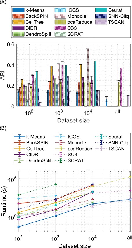
Comparison of clustering performance and scalability. (A) The |$y$|-axis is the ARI of the clustering results on the PBMC dataset. The |$x$|-axis is labeled by the size of the (downsampled) datasets. (B) The |$y$|-axis shows the runtime of clustering the PBMC dataset. The |$x$|-axis is also labeled by the size of the (downsampled) datasets. The curves are truncated if a method is not scalable to a certain size of the dataset.
Figure 1A also shows that |$K$|-means, SC3 and pcaReduce, all of which use |$K$|-means as one of the steps in the clustering, have the largest variance among the multiple runs while the hierarchical clustering methods cellTree, CIDR and DendroSplit, the graph-based clustering method, SNN-Cliq and the density-based clustering method Monocle always returns the same clustering output in the multiple runs. The mixture models, TSCAN and Seurat, and the neural network method, SCRAT also always return the same clustering results indicating that some strategy for obtaining a fixed initialization is used in the implementation.
A further analysis of the results obtained by the clustering techniques shows that hierarchical clustering-based methods exhibit very close mean ARI results. When clustering 1000 cells, we can see that BackSPIN, CIDR, DendroSplit and ICGS have ARIs between approximately 0.25 and 0.3. cellTree, though also based on hierarchical clustering, applies LDA projection of the data, which appears more suitable to the read count data. In terms of partition-based methods, we can see that even though pcaReduce utilizes |$K$|-means as part of its framework, it is able to improve the clustering results with proper use of PCA and the clustering merge strategy. SC3 consensus clustering appears to be a very promising method that combines the advantages of several distance measures and projections. However, the results seem to be unstable when SC3 depends on the SVM to classify more cells, e.g. the result of clustering 10 000 is worse than that of clustering 1000 cells. TSCAN using GMM shows better results than |$K$|-means when using all cells (|$P$| = 0.001 by |$t$|-test), which suggests that the Gaussian modeling may play a positive role in clustering. The implementation of SOM in SCRAT appears to have poor scalability probably due to the large number of gene expression features in the network even though SOM can be trained with stochastic gradient decent. For density-based clustering, Monocle outperforms the other methods by a large margin for clustering 10 000 cells. Moreover, Monocle is relatively scalable with an efficient implementation of density peak clustering by [52]. Finally, even though both Seurat and SNN-Cliq build SNN as the foundation for clustering, Seurat performs better by using the Louvain algorithm instead of clique detection as SNN-Cliq.
This experiment shows that, even though there is a large number of clustering methods specifically designed for scRNA-seq analysis, they show considerably varying results for clustering thousands of cells, and there is still a need for methods that can scale to a large number, such as hundred thousands, or possibly more, rather than using a supervised step.
Clustering multiple cell populations in breast cancer
We downloaded the original dataset from [67] containing 515 cells of 11 patients with breast cancer. The dataset reports TPM values of 25 636 genes, from which we extracted the top 5000 genes with the largest variance in expression. The dataset labels each cell in one of the three groups: immune, stromal or tumor. Because some of the patients do not contain cells of all three types, we utilized 212 cells from 5 patients.
This dataset was used to mainly compare the two methods that are designed to cluster multiple populations, scVDMC [9] and Seurat 2.0, a new version of Seurat [11]. Seurat 2.0 applies pairwise CCA to integrate multiple datasets in a space that maximizes the correlation between their projections. Seurat 2.0 was run with the number of selected genes in |$\{3000,3200,\dots ,5000\}$|, the number of canonical correlation components in |$\{2,\dots ,10\}$|, and resolution in |$\{0.2,0.3,0.4,0.5\}$|. The best result is obtained with the three parameters, 1600, 2 and 0.2, respectively. scVDMC assumes the single-cell populations consist of similar cell types with similar markers but possibly varying expression patterns across the datasets due to some population-specific biological variation. The mathematical optimization framework uses embedded feature selection to look for a small set of shared cell markers while allowing varying expressions of the markers in different populations with a controlled variance. scVDMC was run using initialization by separated |$K$|-means with the parameters |$\lambda $| in |$\{100,200,\dots ,1000\}$|, |$\alpha $| in |$\{1,2,\dots ,6\}$| and |$w$| in |$\{1,2,\dots ,6\}$| (see Equation 1 for the definition of the parameters). The best result was obtained by |$\lambda =1000,\alpha =3,w=3$|.
The two methods were also compared to |$K$|-means and the best performing single-dataset clustering algorithms Monocle, SC3 [26] and cellTree [34] in two scenarios: separated clustering, in which data from each patient is clustered separately; and pooled clustering, in which all the data are combined in a single dataset. Monocle was run with the perplexy = 3 option to avoid error with the |$t$|-SNE. |$K$|-Means was used with Person’s correlation distance, which gives better results than using Euclidean distance on this dataset.
Figure 2 shows the clustering results measured by ARI and running time where each method ran 10 times to obtain the mean and the standard deviation. To measure the ARI, we combined the data of all populations together to consider the agreement between the overall clustering and the true clusters in each population. It is interesting to observe in Figure 2A that the pooled version of SC3, |$K$|-means and cellTree perform much worse than the separated version, strongly indicating that simple pooling is not applicable to the integration of multiple scRNA-seq datasets. We also noticed that scVDMC and Seurat 2.0 both achieved better ARIs, with a mean of |$0.681$| for scVDMC, against a mean of |$0.675$| for Seurat 2.0, than separated |$K$|-means with an ARI of |$0.4742$|. Even though the mean of scVDMC is higher, we can notice that its variance of results is also higher, so that the difference to Seurat 2.0 is not statistically significant ( |$P$| = 0.3511 by |$t$|-test) due to the |$K$|-means initialization in scVDMC. scVDMC has also shown better mean runtime performance than Seurat 2.0 (|$P$| = |$2E-14$| by |$t$|-test), with a mean of 56s against 151s. Overall, the results in this experiment clearly demonstrate the advantage of applying advanced learning methods such as multitask clustering or multi-CCA to integrative clustering of multiple cell populations.
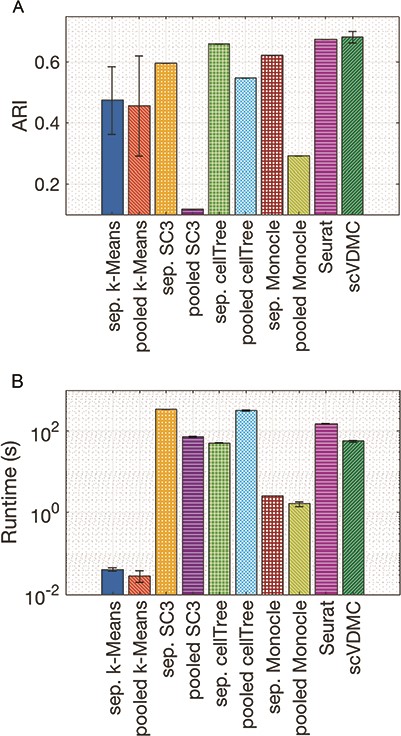
Clustering multiple BRCA cell populations. Comparison of the methods by clustering multiple BRCA cell populations with (A) ARI and (B) running time.
Discussions and conclusions
In the past 6 years, there has been substantial development of clustering algorithms specifically for the analysis of scRNA-seq data. These algorithms aim to tackle challenges inherent in scRNA-seq data, such as cell-specific biases, dropouts and technical noise. Some algorithms have been developed to solve the tasks involving multiple populations of cells [9, 11], detection of rare cell types [14, 22] and pseudotime ordering of cells [34, 61]. Moreover, there is substantial attention given to the development of data preprocessing techniques, such as normalization, dropout imputation, dimension reduction and similarity measures, which contribute to reducing the technical variations before clustering is performed. Together, these advances in computational methods have provided a wide variety of useful tools for clustering analysis of scRNA-seq data.
We also observed that increasing number of studies are in need of more scalable clustering algorithms to transfer the success of single-cell clustering algorithms to larger datasets. The more scalable new scRNA-seq platforms have tremendously reduced the cost and time for cell capture and sequencing and have enabled new studies to utilize a much larger number of single cells, e.g. droplet-based platforms from the 10x Genomics can capture and sequence one million cells for each study [66]. This advance brings new challenges. We observed that most existing tools do not scale well to tens of thousands of cells, which limits the applicability of the algorithms in future studies.
Another limitation of the current methods is related to the opportunities for data integration. The fast growing number of single-cell datasets becoming available in the past few years shows that, soon enough, the vast amount of single-cell data will allow the curation of specific knowledge bases of cell types, cell markers, their expression patterns or even epigenomic features. In addition, there will be single-cell resolution profiling of large patient cohorts such as those in The Cancer Genome Atlas. We have shown that there only exists a limited number of methods for performing single-cell clustering when multiple datasets are combined in a meta-analysis. As the number and size of single-cell datasets continue to grow, advanced data integration methods will be in great need.
In addition to the unsupervised learning methods described in this review, we also noticed an alternative problem formulation that utilizes supervised or semisupervised ideas to perform cell type identification. For example, SC3 [26] package uses supervised learning to assign the remaining cells to the clusters found by consensus clustering, improving the scalability to a larger number of cells. Scmap [68] applies to a scenario where the cell types of a subset of cells are known a priori in a reference dataset and then the cells of unknown cell type from some other dataset are mapped to the most similar group of cell types with the nearest neighbor classification after gene feature selection. In a more general formulation of the problem, a model needs to classify the cells into the known cell types and identify cells of new types to detect new clusters. Clearly, a multistage approach or more advanced modeling technique is necessary.
Finally, more different types of single-cell data have now been collected in addition to RNA expression, such as single-cell epigenomic data [69], single-cell Hi-C genome structures [70, 71] and single-cell DNA sequencing [72]. While some of the clustering methods developed for scRNA-Seq data could also be applicable to some of the new single-cell data types, we expect there will also be substantially new computational development for clustering analysis of the new data types.
The new computational challenges for clustering scRNA-seq data include dropout imputation, rare cell-type detection, integration of multiple single-cell populations, inference of cell developmental trajectory and the evaluation and intepretation of single-cell clusters.
There has been substantial new computational development dedicated to the clustering analysis of scRNA-seq data analysis including clustering techniques, normalization and imputation methods, dimension reduction methods and more advanced learning methods for time series, multiple dataset integration and small cluster detection.
Current clustering methods scale only to scRNA-seq datasets with tens of thousands of cells. More scalable algorithms are necessary to allow applications to target larger scRNA-seq datasets such as possibly as many as 1 000 000 cells generated from droplet-based platforms.
Clustering algorithms, which integrate multiple cell populations and are applicable to the clustering of other types of single-cell (epi)genomic data, are also in great demand to support future analysis of scRNA-seq data from patient cohorts and new types of single-cell data.
Funding
RP is partially supported by the CAPES Foundation, Ministry of Education of Brazil (BEX 13250/13-2).
Raphael Petegrosso is currently a PhD candidate in Computer Science at the University of Minnesota Twin Cities. He received his BS in Computer Engineering from University of Sao Paulo, Brazil. His research interests include network-based learning, semisupervised learning and phenome-genome association analysis.
Zhuliu Li is currently a PhD candidate in Computer Science at University of Minnesota Twin Cities. He received his BE in Electric Engineering from Xidian University, China. His research interests include statistical learning, semisupervised learning, network-based learning and applications in biological networks.
Rui Kuang is an associate professor with Computer Science and Engineering Department at University of Minnesota Twin Cities with joint appointment in Bioinformatics and Computational Biology. His research interests are broadly in biological network analysis, cancer genomics, phenome predictions and machine learning.
References
