


Abstract
Motivation: Estimating differentiation potency of single cells is a task of great biological and clinical significance, as it may allow identification of normal and cancer stem cell phenotypes. However, very few single-cell potency models have been proposed, and their robustness and reliability across independent studies have not yet been fully assessed.
Results: Using nine independent single-cell RNA-Seq experiments, we here compare four different single-cell potency models to each other, in their ability to discriminate cells that ought to differ in terms of differentiation potency. Two of the potency models approximate potency via network entropy measures that integrate the single-cell RNA-Seq profile of a cell with a protein interaction network. The comparison between the four models reveals that integration of RNA-Seq data with a protein interaction network dramatically improves the robustness and reliability of single-cell potency estimates. We demonstrate that underlying this robustness is a correlation relationship, according to which high differentiation potency is positively associated with overexpression of network hubs. We further show that overexpressed network hubs are strongly enriched for ribosomal mitochondrial proteins, suggesting that their mRNA levels may provide a universal marker of a cell’s potency. Thus, this study provides novel systems-biological insight into cellular potency and may provide a foundation for improved models of differentiation potency with far-reaching implications for the discovery of novel stem cell or progenitor cell phenotypes.
Introduction
Over 60 years ago Waddington proposed an epigenetic landscape model of cellular differentiation, whereby cell fate transitions are modeled as canalization events, with stable cell states defining the attractors or basins in this landscape [1, 2]. Focusing on a given cell lineage, a key ingredient of this landscape is the height of the attractor states [3], which is believed to correlate with differentiation potency, i.e. the relative number of downstream cell fate choices a given cell may have. Quantifying the differentiation potency of single cells is a task of critical importance, as it may help estimate potency heterogeneity within otherwise seemingly homogenous cell populations [4], it may facilitate explicit construction of Waddington landscapes [2, 5] and provide an unbiased means of identifying novel stem or progenitor cell phenotypes [6].
Given that mRNA expression levels of genes in a cell may inform on the activity of transcription factors and associated signaling pathways that control pluri-and-multi potency [7], it is reasonable to assume that differentiation potency is encoded by the genome-wide transcriptomic profile of the cell [6, 8–10]. Following this rationale, a number of explicit potency models based on biological principles have been proposed [6, 9–13]. For instance, StemID [6] estimates potency of a cell in terms of its genome-wide transcriptomic entropy, which measures how uniformly expressed the genes are. Because stemness is characterized by large numbers of differentiation expression programs being kept at a low and comparable level of basal activity, this transcriptomic entropy may therefore approximate potency. Another proposed model, called SLICE [9], groups genes into Gene-Ontology (GO) clusters and approximates potency of a cell in terms of a Shannon entropy, defined over gene expression derived activity estimates for each GO cluster: in effect, this measures the degree of uniformity of the GO-cluster activation levels and thus the degree of uniformity in the activation levels of different biological processes in a cell. A third model, called SCENT [10], integrates the single-cell RNA-Seq (scRNA-Seq) profile of a cell with a protein–protein interaction (PPI) network, modeling potency in terms of how efficient signaling can diffuse over the whole network. The efficiency of the diffusion process is estimated by the signaling entropy rate, which is expected to be lower for differentiated cells, since differentiation is accompanied by activation of a specific subnetwork, which in effect draws signaling flux away from other parts of the network [10]. Importantly, SCENT has been shown to estimate potency not only of normal cells, but also of cancer cells allowing putative cancer stem cell phenotypes to be identified [10].
Given the importance of estimating single-cell potency, a comparison of these different potency models is of great interest, and here we do so by performing a comprehensive comparison across a large number of independent scRNA-Seq datasets all profiling normal cells, in order to objectively determine which single-cell potency models are most accurate and robust. We do this in both single-cell as well as bulk-sample settings, while also adjusting for cell-cycle phase, which is a major confounder in scRNA-Seq studies. In performing these comparisons, we also introduce a novel single-cell potency measure, called Markov Chain Entropy (MCE), which like SCENT integrates the scRNA-Seq profile of a cell with a PPI network. Our results highlight that SLICE and StemID are less robust than SCENT/MCE in both single-cell and bulk tissue settings. We provide a detailed explanation and understanding as to the factors driving the increased robustness of MCE and SCENT, revealing that potency can be approximated in terms of the correlation between the transcriptome and connectome.
Materials & Methods
MCE
We here describe the construction of MCE to represent the potency of a sample with a scRNA-Seq or bulk RNA-Seq profile. The construction requires two inputs, i.e. the normalized RNA-Seq profile and a fully connected signaling interaction network between the genes defined in the profile. For the network, we use the PPI network of 8434 proteins from [10]. We note that although in principle we could infer a gene regulatory network from the scRNA-Seq data itself using one of the many available methods [43–47], this does not work as well as using a PPI network, for reasons given later. Given a network/graph |$G = \{V, E\}$| with |$n_V$| nodes in |$V$| and |$n_E$| edges in |$E$|, we model signaling as a particle on the network and let it do discrete-time Markov transition. Denote the transition probability matrix as |$P = \{p_{ij}\}$|, where |$i,j = 1,\dots , n_E$|. We set |$p_{ij}=0$| if there is no edge between two different nodes |$i$| and |$j$|. |$p_{ii}$| can be nonzero and is the probability of the particle staying at node |$i$|. We assume the network has a steady state with invariant distribution |$\boldsymbol{\pi } = (\pi _1, \dots , \pi _{n_V})$| after the particle walks for long enough time. As we shall see below, the invariant measure or steady-state probabilities will be determined from the sample’s gene expression profile.
The first term in Equation (2) is named as the edge entropy (similar to but not the same as the average local entropy/signaling entropy in [10, 42]), and the second term is called the node entropy. Since |$\pi _ip_{ij}$| means the probability (or information flow or actual interaction) transmitted from |$i$| to |$j$| along the directed edge |$(i,j)$| in |$E$|, MCE is indeed the whole entropy of the information flow induced by the Markov chain on the graph or network |$G$|, rather than the entropy rate [10, 42]). Thus, it can be thought as a measurement of the heterogeneity of a network in terms of actual interactions. The more homogeneous of interactions the graph is, the bigger its MCE grows. We think that this intuition can be utilized to characterize the stemness of cells.
Computing MCE from single-cell RNA-seq dataset
Denote the dataset as |$X = \{\boldsymbol{x}^{(1)}, \boldsymbol{x}^{(2)}, \dots , \boldsymbol{x}^{(n)}\}$|, where |$n$| is the sample size, and |$ \boldsymbol{x}^{(i)} $| is a length-|$n_V$| column vector for gene expressions. |$n_V$| is not only the number of genes in consideration but also the counts of nodes in the gene network.
Computing MCE for each sample
i. qThe normalized gene expression |$\boldsymbol{\pi }= \boldsymbol{x}/||\boldsymbol{x}||_{\mathcal{L}_1}$| is the invariant distribution of a discrete-time Markov transition matrix |$P$| on the gene network |$A$|;
ii. Among all the possible transition matrix |$P$| with invariant distribution |$\boldsymbol{\pi }$| and topology |$A$|, we choose the one with the largest entropy.
|$\boldsymbol{\alpha }^{(n)}= 1./(A\boldsymbol{\beta }^{(n-1)})$|;
|$\boldsymbol{\beta }^{(n)}= \boldsymbol{\pi }./(B^{\prime}\boldsymbol{\alpha }^{(n)})$|,
Normalization of MCE
Other entropy indices
Signaling entropy (SCENT)
The main difference between SR and MCE are
i. The adjacent matrix |$A$| has zero diagonal elements in SR, while it has ones in MCE. The basis of SR is interaction between proteins through the law of mass action, while the basis of MCE is a Markov transition on the gene network. The signaling particle in MCE has a probability to stay at one node which is more meaningful.
ii. For MCE, we maximize the entropy to get the most likely transition matrix given a fixed invariant measure. In contrast, when computing SR, the weights of the stochastic matrix |$P$| are precomputed using the law of mass action, which is therefore fixed.
StemID
SLICE
SLICE is another entropy-based index proposed in [9]. Like StemID it does not use a PPI network. Instead, it first clusters genes into |$m$| functional GO clusters, according to their similarity of GO annotation. For each cell |$j$|, SLICE then computes a probability activity score |$p_{j,k}$| for GO-cluster |$k$| in cell |$j$|, by taking the average expression of genes mapping to a given GO-cluster |$k$|. Subsequently, it approximates potency as the Shannon entropy of the activity distribution, i.e. as |$H_j = \mathbb{E}[-\sum _{k=1}^m p_{j,k}\log p_{j,k}]$|, where the expectation is taken over a number of bootstraps. We computed SLICE as described in [10] using the R-functions provided by Guo et al. [9]. We note that, as with StemID, the computation of SLICE entropy is supposed to be done on the unlogged normalized counts. Thus, we used the downloaded normalized count data matrices when estimating SLICE entropy. The expression threshold parameter in SLICE was set to 1 (default value) for all studies, except for Yao1 where the data were already regularized (logged) and where we used a threshold of 0.1. We note that in the Yao1 study data have been renormalized by subsampling single cells to 20 000 unique molecular identifiers (UMIs) [14].
Summary of RNA-Seq experiments used. Table lists the name of the experiment, the type of RNA-Seq data (if single cell or bulk), the species, the total number of profiles (after quality control), the time points or potency states being compared, the cell types being compared, the number of single cells in each comparison group and the reference. Chu1–4 derive from Chu et al., Trapnell derives from Trapnell et al., Treutlein from Treutlein et al., SemrauRB & SemrauSS derive from the RNA Barcoding (RB) and Smart-Seq (SS) scRNA-Seq experiments in Semrau et al., WangNPC derives from Wang et al., YangML derives from Yang et al. and Yao1 derives from a scRNA-Seq experiment that used UMIs, while Yao2 is a corresponding matched bulk RNA-Seq dataset. Abbreviations: Pl, pluripotent; NonPl, non-pluripotent; E,embryonic day; h, hours; d, day, MP, multipotent progenitor; NPC, neural progenitor cell. For instance, for Chu1 set, we tested the alternative hypothesis that the potency measure is higher in the pluripotent cells compared to non-pluripotent cells, and of the 1018 high-quality scRNA-Seq profiles, 374 were pluripotent and 644 were non-pluripotent
| Name | Type | Species | Total number | Comparison | Cell types in comparison | Numbers in comparison | Ref |
|---|---|---|---|---|---|---|---|
| (after QC) | |||||||
| Chu1 | scRNA | Human | 1018 | Pl >NonPl | hESCs to MPs | 374 versus 644 | [38] |
| Chu2 | scRNA | Human | 758 | 0 h >96 h | hESCs to MPs | 92 versus 188 | [38] |
| Trapnell | scRNA | Human | 372 | 0 h >72 h | Myoblasts to skeletal muscle | 96 versus 84 | [29] |
| Treutlein | scRNA | Mouse | 201 | E14 >Adult | Lung Differentiation | 45 versus 46 | [39] |
| SemrauRB | scRNA | Mouse | 425 | 0–12 h >96 h | hESCs to MPs | 175 versus 25 | [40] |
| SemrauSS | scRNA | Mouse | 292 | 0 h >48 h | hESCs to MPs | 75 versus 61 | [40] |
| WangNPC | scRNA | Human | 483 | 0–1 d >30 d | NPCs to Neurons | 158 versus 81 | [17] |
| YangML | scRNA | Mouse | 447 | E10 >E17 | Liver Differentiation | 54 versus 70 | [16] |
| Yao1a | scRNA | Human | 2684 | 0 d >26 d | hESCs to NPCs | 40 versus 595 | [14] |
| Yao1b | scRNA | Human | 2684 | 0 d >54 d | hESCs to Neurons | 40 versus 765 | [14] |
| Yao1c | scRNA | Human | 2684 | 26 d >54 d | NPCs to Neurons | 595 versus 765 | [14] |
| Chu3 | bulkRNA | Human | 19 | Pl >NonPl | hESCs to MPs | 7 versus 12 | [38] |
| Chu4 | bulkRNA | Human | 15 | 12/24 h >72/96 h | hESCs to definite endoderm | 6 versus 6 | [38] |
| Yao2a | bulkRNA | Human | 33 | 0–9 d >26 d | hESCs to NPCs | 12 versus 6 | [14] |
| Yao2b | bulkRNA | Human | 33 | 0–9 d >54 d | hESCs to Neurons | 12 versus 4 | [14] |
| Yao2c | bulkRNA | Human | 33 | 26 d >54 d | NPCs to Neurons | 6 versus 4 | [14] |
Single-cell and bulk RNA-Seq datasets
In total, we used scRNA-Seq datasets derived from nine independent studies. Two of these studies contained matched bulk RNA-Seq data. From all of these scRNA-Seq studies, we devised 11 independent analyses, comparing in each one cells of high potency to cells of low potency, assessing the different potency measures in their ability to discriminate these cell types. In the case of bulk RNA-Seq data, we devised five independent comparisons from the two studies with bulk RNA-Seq data. Table 1 gives a brief summary of the 11 independent comparisons performed on scRNA-Seq data and the five performed using bulk RNA-Seq data. A more detailed description of the datasets is listed below:
Chu et al. datasets 1–4: These datasets were derived from [38]. There are four experiments named Chu1, Chu2, Chu3 and Chu4. Chu1 dataset contains scRNA-Seq data for 1018 single cells, which is composed of 374 hESCs (human embryonic stem cells, 212 from H1 cell line and 162 from H9 cell line), 173 NPCs (neuronal progenitor cells, ectoderm derivatives), 138 DECs (definitive endoderm cells, endoderm derivatives), 105 ECs [endothelial cells, mesoderm progenitors (MPs)/derivatives], 69 TBs (trophoblast-like cells, extraembryonic derivatives) and 159 HFFs (human foreskin fibroblasts). The hESCs are pluripotent (|$n=374$|) and the others are non-pluripotent (|$n=644$|). Chu2 dataset is a time-course differentiation of single cells, in which hESCs were induced to differentiate into DECs, via a mesoendoderm intermediate. The time points cover before induction at |$t=0$| h (|$n=92$|) and after induction at |$t = 12$| h (|$n=102$|), |$t=24$| h (|$n=66$|), |$t=36$| h (|$n=172$|), |$t=72$| h (|$n=138$|) and |$t=96$| h (|$n=188$|). There are 758 single cells in total. Chu3 dataset is from bulk samples. There are 19 bulk samples, which have seven samples for hESCs, two for NPCs, two for TBs, three for HFFs, three for ECs (MPs) and two for DECs. Chu4 is the time-course experiment of 15 bulk samples, consisting of three samples for each of five time points (12 h, 24 h, 36 h, 72 h and 96 h). Normalized data were downloaded from Gene Expression Omnibus (GEO) under accession number GSE75748 (files: GSE75748-bulk-cell-type-ec.csv, GSE75748-sc-cell-type-ec.csv, GSE75748-bulk-time-course-ec.csv, GSE75748-sc-time-course-ec.csv).
Trapnell et al. dataset: This scRNA-Seq dataset was derived from [29]. It represents a time-course differentiation experiment of human myoblasts into human skeletal muscle cells. Human myoblasts were induced at |$t=0$| h (|$n=96$|). Samples were also taken at |$t=24$| h (|$n=96$|), |$t=48$| h (|$n=96$|) and |$t=96$| h (|$n=84$|) after induction. There are 372 single cells in total. Normalized data were downloaded from GEO under accession number GSE52529 (file: GSE52529-fpkm-matrix.txt).
Treutlein et al. dataset: This dataset was derived from [39]. The experiment took samples from the developing mouse lung epithelium at embryonic days E|$14.5$| (|$n=45$|), E|$16.5$| (|$n=27$|), E|$18.5$| (|$n=83$|) and adulthood (|$n=46$|), totalling 201 single cells. Normalized data were downloaded from GEO under accession number GSE52583 (file: GSE52583.Rda).
SemrauRB and SemrauSS datasets: The two datasets named SemrauRB and SemrauSS were derived from [40], a study of retinoic acid (RA)-driven differentiation of pluripotent mouse embryonic stem cells (mESCs) to lineage commitment. SemrauRB used a recently developed Single Cell RNA Barcoding and Sequencing method (SCRB-seq) and consists of 425 single-cell samples taken at nine time points during mouse embryonic differentiation. There were 53 single cells taken at 0 h. After all-trans RA exposure, 73 samples were taken at 6 h, 49 samples at 12 h, 27 samples at 24 h, 72 samples at 36 h, 43 samples at 48 h, 54 samples at 60 h, 29 samples at 72 h and 25 samples at 96 h. To increase power and because exit from pluripotency occurs after 12 h [40], all cells from 0–12 h were considered to be pluripotent. SemrauSS uses a different scRNA-Seq technology (SMART-seq). A total of 292 single cells were taken at four time points (75 samples at 0 h, 75 samples at 12 h, 81 samples at 24 h and 61 samples at 48 h). Normalized data were downloaded from GEO under accession number GSE79578 (files: GSM2098545-scrbseq-2i.txt, GSM2098550-scrbseq-48h.txt, GSM2098555-smartseq-12h.txt, GSM2098546-scrbseq-6h.txt, GSM2098551-scrbseq-60h.txt, GSM2098556-smartseq-24h.txt, GSM2098547-scrbseq-12h.txt, GSM2098552-scrbseq-72h.txt, GSM2098557-smartseq-48h.txt, GSM2098548-scrbseq-24h.txt, GSM2098553-scrbseq-96h.txt, GSM2098549-scrbseq-36h.txt, GSM2098554-smartseq-2i.txt).
Wang et al. dataset: This dataset was derived from [17], a study of non-directed differentiation over a 30-day period of neural progenitor cells (NPCs) into developing neurons, with the NPCs derived from hESCs. After quality control, there were 483 usable single cell samples describing the differentiation from NPCs (at day 0) to neurons and other differentiated cell-types. Cell numbers were 80 at day 0, 78 at day 1, 85 at day 5, 80 at day 7, 79 at day 10 and 81 at day 30. Normalized data were downloaded from GEO under accession number GSE102066 (file: GSE102066-normalized-counts.experiment1.DataMatrix.txt).
Yang et al. dataset: This scRNA-Seq dataset was derived from [16], a study of differentiation of mouse hepatoblasts into hepatocytes and cholangiocytes. After quality control, 447 single-cell samples were taken during embryonic development. There are 54 single cells at embryonic day 10.5 (E10.5), 70 at E11.5, 41 at E12.5, 65 at E13.5, 70 at 14.5, 77 at 15.5 and 70 at E17.5. Normalized data were downloaded from GEO under accession number GSE90047 (file: GSE90047-Single-cell-RNA-seq-TPM.txt).
Yao et al. datasets 1–2: This scRNA-Seq dataset (Yao1) was obtained by using a method based on multiplexed single-cell RNA-seq (CelSeq) and UMIs [14]. Cel-Seq was used to profile cells at multiple time points (days 0, 12, 19, 26, 40 and 54) in a study of differentiation of hESCs into cortical and non-cortical progenitor and finally into neurons. After quality control, there were 2684 single cells: 40 hESCs, 504 collected at day 12, 278 at day 19, 595 at day 26, 502 at day 40 and 765 at day 54. Progenitor expansion into neurons occurred at day 26. Normalized data were downloaded from GEO under accession number GSE86977 (file: GSE86977-UMI-20K.2684.csv). In addition, we also analyzed a matched bulk RNA-Seq dataset (Yao2) from the same study, encompassing a total of 33 samples: five hESC samples (day 0), three samples at day 6, four samples at day 9, six samples at day 12, five samples at day 19, six samples at day 26 and four samples at day54. Normalized data were downloaded from GEO under accession number GSE86985 (file: GSE86985-trueseq.tpm.csv).
Further processing and quality control analysis
We used the following general procedure to further assess quality and further normalize the provided scRNA-Seq data. First, in all cases, we computed the coverage per single cell, i.e. the number of genes with normalized counts (e.g. transcripts per million (TPM) fragment reads per kilobase exon per million (FPKM)) above zero. Any single cell with less than |$10\%$| coverage was removed. Next, we quantile normalized (QN) the resulting dataset to remove potential batch effects. For most datasets, we then renormalized the minimum read count to 1, i.e. any normalized count less than 1 was renormalized to 1. We justify this on the basis that the normalized counts of 1 and 0 are effectively indistinguishable. The threshold of 1 was derived by inspection of the distribution of normalized counts. After QN, we log2-transformed the data with an offset value of 0.1 added before log-transformation. The offset was added in order to ensure that the minimum value after log-transformation would not be 0, but a nonzero value (typically |$\log _2{1.1}\approx 0.13$|). We did not want zeroes in our final matrix to avoid singularities in the computation of the signaling entropy rate used in SCENT. The log-transformation was done to stabilize the variance and regularize the effects of outliers. Next, in the case of human data, we mapped gene symbols to Entrez gene IDs (if not annotated to Entrez gene IDs already) and finally averaged any entry mapping to the same Entrez gene ID. In the case of mouse, we first obtained the human homologs using the annotationTools Bioconductor package (http://www.bioconductor.org) and finally mapped to human Entrez gene IDs. The typical range of a resulting data matrix was then typically 0.13 to approximately 16.
We note that the Yao1 scRNA-Seq dataset used CelSeq-technology and UMIs and was normalized using a different procedure as described in [14]. For this dataset, we therefore used a slightly different choice of thresholds. First, the data downloaded was already on a log-scale, but still with a few significant outliers: thus, we regularized the data further by setting any values larger than 16 to 16. We then performed QN and finally any value less than 1 was set to a value of 0.1 (in order to remove zeroes from the data matrix).
The above procedure resulted in data matrices defined over human Entrez gene IDs and single cells of following dimensions: Chu1 (18935 genes, 1018 single cells), Chu2 (18935 genes, 758 single cells), Chu3 (18935 genes, 19 bulk samples), Chu4 (18935 genes, 15 bulk samples), Trapnell (22351 genes, 372 single cells), Treutlein (12413 genes, 201 single cells), SemrauRB (13 755 genes, 425 single cells), SemrauSS (13663 genes, 292 single cells), WangNPC (8242 genes, 483 single cells), YangML (16119 genes, 447 single cells), Yao1 (22113 genes, 2684 single cells) and Yao2 (19 659 genes, 33 bulk samples).
Evaluation framework
In order to compare the different potency measures (described in the next subsections), we assessed their ability to discriminate single cells (and bulk samples) that ought to differ substantially in terms of their potencies. We reasoned that potency measures which would fail to discriminate such cell types would be less preferable than those that are more robust. For each of the studies, we therefore devised comparisons between cell types (or bulk samples) where typically we would expect to see a big difference in potency, so that it is reasonable to assume that higher Area Under the Curves (AUCs) (discriminatory ability) and more significant P-values (as derived using one-tailed Wilcoxon rank sum tests) would indicate better potency measures. For the scRNA-Seq datasets, we devised a total of 11 independent comparisons, where the specific cell types being compared and the corresponding cell numbers are given in Table 1. Below, we briefly summarize the comparisons.
In Chu1, we chose to compare the pluripotent hESCs to all progenitor and non-pluripotent cell types. In Chu2, we compared the hESCs at time 0 to the final time point (96 h) corresponding to definite mesoderm/endoderm (i.e. non-pluripotent). For the corresponding bulk sets Chu3 and Chu4, we chose the same groups, although for Chu4 only 12 h and 24 h were available to represent the pluripotent state, so for Chu4 we compared 12 h/24 h to 72 h/96 h, which yielded six samples in each group. Only using 12 h and 96 h would result in too few samples. We also note that the transition to the definite mesoendoderm occurs at 72 h and beyond. In Trapnell, we compared the myoblasts at 0 h to the differentiated skeletal muscle cells at 72 h. In Treutlein, we compared embryonic day E14 to the adult differentiated cells. In SemrauRB, because exit from pluripotency occurs after 12 h and because cell numbers at each time point were fairly low, we compared all cells harvested at 0, 6 and 12 h to those harvested at 96 h. In SemrauSS, we compared cells at 0–48 h. In WangNPC, we compared neural progenitors at 0 and 1 day to differentiated neural cells at 30 days. We deemed safe to bunch together 0 and 1 day cells as differentiation occurred much later in the assay and to increase cell numbers for the more potent NPC phenotype. In YangML, we compared embryonic day 10 (E10) to E17 single cells. In Yao1, we devised three separate comparisons, because in this study there were many single cells and because the nature of the experiment allowed precise definition of three potency states: hESCs at day 0, cortical and non-cortical progenitors at day 26 and differentiated neurons at 54 days. Thus, in Yao1a we compared day 0 to day 26, in Yao1b, we compared day 0 to day 54, and in Yao1c we compared day 26 to day 54. For the corresponding bulk sample study, Yao2, we also performed three comparisons, but in order to increase sample numbers we considered the pluripotent state to also include day 9 samples, which is justified based on the findings of the original publication [14].
Adjusting for cell-cycle phase
Differences in cell potency between groups could be confounded by differences in the proportion of cycling versus non-cycling cells. For each single cell we thus computed two cell-cycle scores (one for the G1-S and the other for the G2-M phase), using the procedure described in [10, 41]. Because the relation between potency and cell-cycle scores could be highly nonlinear (as described in [10]), linear adjustment procedures are inappropriate. Another approach to compare potency of cell types, adjusted for cell cycle, would be to set a threshold on the scores and only use cells with cell-cycle scores below a given threshold. However, these thresholds may be study-specific, and we found that if we were to use the same threshold for all studies, that this may lead for specific studies to highly unequal numbers of low-cycling cells in each comparison group or to effectively no cells in a given group. For instance, in some studies we find that all single hESCs exhibit relatively high-cycling scores. This indicates that disentangling cell-cycle effects and potency is extremely difficult, if not impossible, and may also be strongly dependent on the experimental details (e.g. culture conditions of cells, etc.). Thus, we decided on a different approach which would allow us to compare cell types, while adjusting for cell-cycle phase as much as possible. Specifically, for each study and cell type of interest, we chose a lower quantile of cell-cycle scores based on the scores of all cells within that cell type. Doing so, ensure that we are comparing sufficient numbers of single cells within each group, but also that we are using the lowest-cycling cells within each group. The quantiles were chosen to ensure sufficient numbers of cells in each comparison group. We note that since there are two cell-cycle scores, which we performed this operation on G1-S and G2-M separately, subsequently only using the single cells that were in the lower-defined quantile for both phases. Thus, absolute cell numbers could be low for some studies, but with the chosen quantiles enough cells were being compared to achieve potential statistical significance. The quantiles chosen, the number of low-cycling single cells in each comparison group and the results obtained are listed in Table S2.
Construction of a model landscape
Results
Modeling single-cell potency as the graph entropy of a Markov chain process
The measured mRNA expression profile of a cell can be interpreted as the net result of a complex signaling process that takes place in the cell. Assuming an interaction network (e.g. a PPI network), one may thus attempt to model a given signaling process in terms of a Markov chain that is consistent with the observed expression profile of the cell (Methods, Figure 1A).
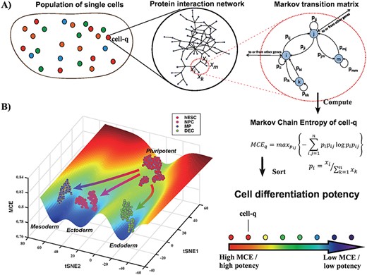
Markov-Chain Entropy (MCE) for quantifying single-cell potency in Waddington’s landscape. (A) The key assumption underlying the estimation of MCE is that the measured gene expression profile |$\boldsymbol{x} = (x_1, \dots , x_n)$| of a cell q is the end result of an unknown Markovian signaling process in the cell, which however we can try to estimate by using a network model of signaling interactions. This network imposes constraints on the space of all possible Markov transition matrices, and MCE is estimated from the one maximizing the Shannon entropy of the Markov process. Having estimated MCE for each single cell, we can then sort them according to their MCE, which we posit is a proxy for cell potency. (B) An example of a Waddington epigenetic landscape for the Chu1 et al. dataset (Table 1), depicting four main attractor states, representing hESCs (pluripotent), NPCs (ectoderm, multipotent), MPs (mesoderm, multipotent) and definite endoderm progenitor cells (DECs, endoderm, multipotent). The z-axis labels the MCE values of over 1000 single cells representing these four cell types, whereas the y-axis and x-axis label the projections inferred using t-SNE.
For each Markov-chain process one can further define an associated graph entropy, here termed MCE, that measures the overall uniformity of the signaling fluxes in the network (Methods, Figure 1A). We posited that among all Markov chains consistent with the observed expression profile, the one maximizing the graph entropy could provide us with an estimate of single-cell potency (Methods, Figure 1A). To understand this, we note that higher entropy means a more uniform Markov chain signaling process on the network, allowing signaling information to diffuse more efficiently. Thus, since a terminally differentiated cell (a cell of lowest potency) is characterized by the activation of specific signaling subnetworks (i.e. signaling pathways), it is plausible that this nonuniformity can be detected in terms of a lower MCE.
Comparison of single-cell potency measure reveals robustness of MCE and SCENT
To compare the different single-cell potency models we devised an evaluation framework, designed to be as objective as possible: we reasoned that although a population of seemingly equally potent single cells may not be entirely so due to inter-cellular heterogeneity a reliable potency measure should be able to nevertheless discriminate single-cell populations that differ significantly in terms of differentiation potency. For instance, a robust single-cell potency measure should be able to discriminate pluripotent from non-pluripotent cell populations or cells at the start and endpoints in time-course differentiation experiments. Thus, we assembled a collection of nine scRNA-Seq experiments, encompassing a total of approximately 6700 high-quality scRNA-Seq profiles, from which we devised 11 independent comparisons between cell types that ought to differ significantly in terms of differentiation potency (Methods, Table 1).
To each of these datasets, we applied the three previously proposed single-cell potency models (StemID [6], SLICE [9] and SCENT [10]), as well as MCE.
We first considered a time-course differentiation experiment in which hESCs were induced to differentiate into cortical NPCs and finally into neurons over a 54 day period, with scRNA-Seq measurements taken at six time points, encompassing a total of 2684 single cells [14]. While MCE and SCENT showed the expected gradual decrease of potency with differentiation time point, StemID exhibited a less significant pattern, while SLICE did not exhibit a decrease (Figure 2A).
![Comparison of discrimination accuracy of single-cell potency measures across scRNA-Seq datasets. (A) For the scRNA-Seq dataset (Yao et al. [14]), which profiled over 2600 cells in a time-course differentiation of hESCs (day 0) to NPCs (day 26) and finally to terminally differentiated neurons (day 54), we show corresponding violin plots of the predicted potencies at each measured time point and for the four different potency measures (SLICE, StemID, MCE and SCENT), as indicated. The number of cells at each time point is given below violins. (B) Left panel: Barplots compare the AUCs of the four different single-cell potency measures across 11 independent comparisons drawn from nine independent scRNA-Seq experiments (see Table 1 for definitions of cell types being compared). The AUCs reflect the measure’s discrimination accuracy of single cells that ought to differ in terms of differentiation potential and can be derived from the statistic of a Wilcoxon rank sum test. P-values are also derived from a one-tailed Wilcoxon rank sum test comparing cell types. Right panel: Heatmap of meta-analysis P-values comparing single-cell potency measures to each other. P-values estimated from a paired one-tailed Wilcoxon rank sum test over the 11 independent comparisons. In the heatmaps, the P-value entry for column i and row j is for testing the alternative hypothesis that method in row j has higher AUC values than method in column i. (C) As (B), but now adjusting for cell-cycle phase, i.e. using only the cells with the lowest-cycling scores in each comparison group.](https://oup.silverchair-cdn.com/oup/backfile/Content_public/Journal/bib/21/1/10.1093_bib_bby093/4/m_bby093f2.jpeg?Expires=1749164420&Signature=x3~mQfIW7Y7jyLRrhxowpxIxOql71V0IYhXmX0T~gEUks6magGrbZZQibJXT5o1-FIL0eIUpqDbMILYRsTqBDEzQVXQG14UOn5i8FBV3cVBBm~TMHUMQHEZdYY9A-ZMl6QTxOXTPw01OYFGiEs3tzRh7Qz9UXfNhUMKYOLmSnbM0JUmY1FDRanETo2il0LQtFB0zib7PiXcDGf9Yp-12jpVIhlUIHXVW0qoqo80LTFH0RdfRdQVmQg7H~lNEXp0aIh~bpVRvNPVGmRm8vxDYCdsh3bs88gi7KDnCf8HwdopVSwC6oLFVSKm-LMFYNiJ-lSuNTJuyGDYshu2-d0VZyw__&Key-Pair-Id=APKAIE5G5CRDK6RD3PGA)
Comparison of discrimination accuracy of single-cell potency measures across scRNA-Seq datasets. (A) For the scRNA-Seq dataset (Yao et al. [14]), which profiled over 2600 cells in a time-course differentiation of hESCs (day 0) to NPCs (day 26) and finally to terminally differentiated neurons (day 54), we show corresponding violin plots of the predicted potencies at each measured time point and for the four different potency measures (SLICE, StemID, MCE and SCENT), as indicated. The number of cells at each time point is given below violins. (B) Left panel: Barplots compare the AUCs of the four different single-cell potency measures across 11 independent comparisons drawn from nine independent scRNA-Seq experiments (see Table 1 for definitions of cell types being compared). The AUCs reflect the measure’s discrimination accuracy of single cells that ought to differ in terms of differentiation potential and can be derived from the statistic of a Wilcoxon rank sum test. P-values are also derived from a one-tailed Wilcoxon rank sum test comparing cell types. Right panel: Heatmap of meta-analysis P-values comparing single-cell potency measures to each other. P-values estimated from a paired one-tailed Wilcoxon rank sum test over the 11 independent comparisons. In the heatmaps, the P-value entry for column i and row j is for testing the alternative hypothesis that method in row j has higher AUC values than method in column i. (C) As (B), but now adjusting for cell-cycle phase, i.e. using only the cells with the lowest-cycling scores in each comparison group.
Comparing hESCs to NPCs at day 26 (Figure 2A, Yao1a in Table 1) and separately hESCs to differentiated neurons at day 54 (Figure 2A, Yao1b in Table 1) revealed that SCENT and MCE could discriminate cells with almost perfect accuracy (see Yao1a and Yao1b in Figure 2B, Supplementary Table S1). As expected the difference in potency between NPCs and neurons (Yao1c in Table 1) was less strong but still significantly stronger than the differences predicted by StemID or SLICE (see Yao1c in Figure 2B, Supplementary Table S1). As assessed over the 11 independent comparisons (Table 1, Supplementary Figure S1), we observed that MCE and SCENT outperformed the other two (SLICE and StemID), also when adjusted for cell-cycle phase (Figure 2B and C, Supplementary Tables S1 and S2, Methods). In 9/11 comparisons, MCE and SCENT were better than StemID, and in all 11 better than SLICE. The better performance of MCE and SCENT was statistically significant under a paired Wilcoxon test over the 11 comparisons (Figure 2B and C).
MCE and SCENT outperform other potency models on bulk RNA-Seq data
Since potency is also a property of a cell population [10, 15], any robust measure of single-cell potency should, in principle, also work for bulk samples since a bulk RNA-Seq profile is effectively an average over single cells [8]. We observed that only SCENT and MCE exhibited a robust performance on bulk samples (Supplementary Table S3), in line with the results obtained on scRNA-Seq data. Thus, based on the comparative analysis performed here, we conclude that SCENT and MCE currently provide the more robust measures of cell potency, and therefore advocate their use for explicit, unbiased construction of Waddington landscapes. For instance, we applied MCE to the Chu1 dataset (Table 1, Methods), in combination with t-SNE [48], to construct a Waddington epigenetic landscape encompassing four attractor states, representing pluripotent hESCs and multipotent (i.e. non-pluripotent) progenitors from the three main germ layers: ectoderm, mesoderm and endoderm (Figure 1B).
MCE correctly predicts differentiation time points
To further validate MCE we applied it to two different time-course differentiation experiments, generating three-dimen-sional representations of cell-lineage trajectories. For an embryonic time-course differentiation experiment of mouse hepatoblasts into hepatocytes and cholangiocytes (Yang et al., Table 1), MCE predicted separation after embryonic day 13 (Figure 3A), consistent with the findings of [16]. When applied to a 30 day time-course differentiation experiment of neural progenitor cells into neurons (Wang et al., Table 1), MCE correctly predicted a gradual decrease in potency (Figure 3B, Supplementary Figure S1).
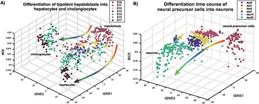
Three-dimensional representation of single-cell differentiation trajectories according to MCE. (A) Differentiation landscape of hepatoblasts. Figure depicts a three-dimensional representation of single cells in an embryonic differentiation time course of mouse hepatoblasts into hepatocytes and cholangiocytes (Yang et al.), as indicated. The MCE potency estimate labels the z-axis, whereas the x and y axes correspond to the tSNE components. Observe how the model predicts separation/differentiation into hepatocytes and cholangiocytes at embryonic day 13 (E13) in line with the results of Yang et al.(B) Differentiation landscape of neural precursor cells into neurons. Figure depicts a three-dimensional representation of single cells in a differentiation time course of human neural precursor cells (day 0) into neurons (day 30) (Wang et al.), as indicated. Observe how MCE correctly predicts a gradual decrease in potency with time of differentiation.
Thus, these applications illustrate that the estimate of cell potency as given by MCE is able to track gradual changes in potency with time, as well as specific time points at which differentiation into distinct cell fates occur.
Cellular potency encoded by the Pearson correlation of transcriptome and connectome
In order to understand the increased robustness of MCE and SCENT over StemID and SLICE, we note that both MCE and SCENT integrate the scRNA-Seq data with orthogonal (i.e. completely independent) connectivity information as derived from a PPI network [10] (Figure 1A, Methods). While such networks are mere caricatures of the complex spatially and temporally dependent signaling processes that take place in a cell, it is plausible that there are specific robust network features that could contribute to the observed robustness of the MCE and SCENT measures. For instance, the difference in connectivity between a hub and a low-degree node is likely to be true irrespective of the PPI network considered and also likely to hold in a wide range of different cell types and biological contexts where both proteins are expressed at similar levels. To explore this, we first verified that the network is indeed a critical feature underlying the robustness of MCE as a potency measure. Specifically, using the neural progenitor to neuron differentiation experiment from Wang et al. [17], we observed how the discrimination accuracy of MCE decreased significantly upon permuting the expression values over the nodes in the network (Figure 4A–C).
![Integration with network information underpins the association of MCE with cell potency. (A) Violin plots of the observed MCE values for NPCs and terminally differentiated neurons (scRNA-Seq data from Wang et al.). P-value derives from a one-tailed Wilcoxon rank sum test. (B) As (A), but now for a random permutation of the expression values over the network, leading to a reduced discrimination accuracy. (C). Comparison of the AUC discrimination measure for the observed case [depicted in (A)] and for 100 distinct permutations. P-value is an empirical one comparing the observed AUC to those from the 100 permutations. (D) MCE (y-axis) is approximated reasonably well by the Pearson Correlation Coefficient (PCC) between the transcriptome and connectivity/degree profile of the network (x-axis). $R^2$ value is given. (E) Boxplots of t-statistics of differential expression between NPCs and neurons (y-axis) against node degree (x-axis), with larger degrees binned into equal-sized groups. Green dashed line denotes the line t = 0. Red line is that of a linear regression. PCC is the Pearson correlation between the t-statistics and node degree. We also give the P-value for the linear regression.](https://oup.silverchair-cdn.com/oup/backfile/Content_public/Journal/bib/21/1/10.1093_bib_bby093/4/m_bby093f4.jpeg?Expires=1749164420&Signature=eTMAqcBooMMpnqgeWKOKv~vRhcoOCqTLzh~Fg4zX10QJ~McFmjDhpYDX~pNXWYBz66jPSAMxkK6JfmPeE7PkRUAAaxG7OUMjpvCuSJkk0gRxZEkGwg7mDw8pme-ItjFa8hZ9tS8e9hnQJ9veQqz02t6kkuONAci6~DcqLq4gKfhHzkSuEX~R4Upd~vGhu6k2ntPoqoy53d4UMy3GccrBF5Zrj-Qh9Y1MhawLCZeo-~Qlg0ZCGq8oXfKvYoNFOfr5o6vJOhKDuptGVIqkmB0WaCTjZtsEwlkPbmG1cDE-6JyQwemGMWMTMFKoKRtO1dQOGldR9hP6~00eGhbslLhKow__&Key-Pair-Id=APKAIE5G5CRDK6RD3PGA)
Integration with network information underpins the association of MCE with cell potency. (A) Violin plots of the observed MCE values for NPCs and terminally differentiated neurons (scRNA-Seq data from Wang et al.). P-value derives from a one-tailed Wilcoxon rank sum test. (B) As (A), but now for a random permutation of the expression values over the network, leading to a reduced discrimination accuracy. (C). Comparison of the AUC discrimination measure for the observed case [depicted in (A)] and for 100 distinct permutations. P-value is an empirical one comparing the observed AUC to those from the 100 permutations. (D) MCE (y-axis) is approximated reasonably well by the Pearson Correlation Coefficient (PCC) between the transcriptome and connectivity/degree profile of the network (x-axis). |$R^2$| value is given. (E) Boxplots of t-statistics of differential expression between NPCs and neurons (y-axis) against node degree (x-axis), with larger degrees binned into equal-sized groups. Green dashed line denotes the line t = 0. Red line is that of a linear regression. PCC is the Pearson correlation between the t-statistics and node degree. We also give the P-value for the linear regression.
Since the connectivity (or degree) profile is one of the most fundamental properties of a network, we posited that MCE might be approximated by the Pearson correlation between the transcriptome and connectome. We verified that approximately 70|$\%$| of the variance in MCE can be explained by a linear correlation between transcriptome and connectome (Figure 4D). In line with this, we observed that t-statistics of differential expression between NPCs and differentiated neurons were generally positive (i.e. higher expression in NPCs compared to neurons) for network hubs, while low-degree nodes did not exhibit any preference for over or underexpression (Figure 4E). We verified that all of these patterns were a systemic feature, observed in effectively all major datasets analyzed here (Supplementary Figures S2–S10). Specifically, (i) the discrimination accuracy of MCE drops significantly upon permuting expression values over the network nodes, confirming the importance of the network; (ii) the Pearson correlation between trancriptome and connectome explains a significant proportion of the variance in MCE; and (iii) differentiation potency is encoded by a positive correlation between transcriptome and connectome with network hubs always preferentially overexpressed in the cells of higher potency (Supplementary Figures S2–S10).
Biological significance of overexpressed network hubs
In order to gain a better understanding of the above phenomenon, we performed a Gene-Set-Enrichment-Analysis (GSEA) on the network hubs overexpressed in more potent cells. Specifically, we considered the comparison between hESCs and NPCs, as there were two independent scRNA-Seq datasets available (Chu1, Yao1 and Table 1) to assess overall robustness of our findings. Focusing first on Yao1 et al., we verified that network hubs do indeed exhibit preferential overexpression in hESCs compared to NPCs (Figure 5A), a result also evident in Chu1 et al. (Figure 5B).
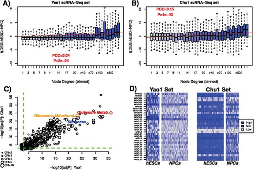
Ribosomal mitochondrial genes enriched for overexpressed network hubs. (A) Boxplots of t-statistics of differential expression between hESCs and NPCs (y-axis) in Yao1 dataset, as a function of node degree (x-axis). Green dashed line indicates the line t = 0, whereas the red line is that of least squares regression fit. Associated PCC and P-value are given. (B) As (A), but now for Chu1 et al. dataset. (C) Scatterplot of the |$-\log _{10}$| adjusted P-values of enrichment of the top-ranked 500 biological terms in Yao1 et al. (x-axis) against their corresponding |$-\log _{10}$| adjusted P-values in Chu1 et al. (y-axis). In color we highlight three biological terms related to metabolism, ribosomal mitochondrial proteins and stemness. The sizes of the circles indicate the average odds ratio over the two datasets. (D) Heatmap of gene expression values for 32 genes encoding mitochondrial ribosomal proteins in the two scRNA-Seq datasets, stratified by hESCs and NPCs. Observe how these 32 genes are more consistently overexpressed in hESCs compared to NPCs.
Performing differential expression analysis using an empirical Bayes framework [18], we next ranked all network hubs (defined as those with a degree |$\geq 90$|) according to overexpression in hESCs and then again by underexpression. Of the 1406 hubs, 376 and 102 were significantly overexpressed and underexpressed (adjusted P-value |$< 0.05$|), respectively. Performing GSEA [19] on the overexpressed subset revealed a striking and highly significant enrichment for genes encoding stemness, glutamine metabolism and mitochondrial ribosomal proteins (Supplementary Table S4) with top-ranked biological terms highly reproducible between the two independent scRNA-Seq datasets (Figure 5C). This enrichment was only observed for overexpressed network hubs and not for underexpressed ones (Supplementary Figure S11, Supplementary Table S5). Corresponding heatmaps of gene expression confirmed the overexpression of mitochondrial ribosomal genes in both scRNA-Seq datasets (Figure 5D). These findings are highly consistent with those of a recent study, which showed that suppression of transcription of ribosomal genes and upregulation of lineage-specific factors in hematopoiesis coordinately control lineage differentiation [20].
Discussion
We have here performed a comprehensive comparison between four different single-cell potency models. All four potency models use a notion of entropy to quantify differentiation potency but differ significantly in terms of their construction and meaning. The transcriptomic entropy used in the StemID algorithm only uses information from the scRNA-Seq profile and approximates potency in terms of the uniformity of gene expression levels. In contrast to StemID, SLICE, SCENT and MCE use additional information to define entropy and potency. In the case of SLICE, activity estimates are obtained for clusters of genes with similar GO annotations, by averaging expression values of genes in a given cluster, and with the entropy and potency subsequently being calculated over these cluster activity estimates. The hypothesis underlying SLICE is that a more uniform activity distribution corresponds to a more potent cell. SCENT and MCE differ from SLICE in that they don’t use GO-terms but instead integrate scRNA-Seq data with a model interaction network. In the case of SCENT, a weighted interaction network is constructed in a cell-specific manner, with the weights reflecting interaction probabilities derived from the gene expression profile of the cell. These weights define a stochastic matrix, from which a signaling entropy can then be defined, which quantifies the efficiency of diffusion of signaling over the whole network. This entropy may approximate potency if the diffusion is less efficient in more differentiated cells, which could happen as a result of activation of specific subnetworks which draws in signaling flux at the expense of diffusing to other parts of the network. While MCE also integrates the scRNA-Seq data with an interaction network, it does not specify the signaling process but infers it from the data itself using the observed gene expression profile of the sample as the invariant steady-state measure of the Markov chain. In this model, potency is the graph entropy of this inferred Markov chain process, measuring the uniformity or promiscuity of the overall process on the network. As with SCENT, the underlying hypothesis is that a more potent cell exhibits a more promiscuous signaling pattern. Although information and signaling flow is most often understood in the context of regulatory transcription factor gene target networks, which are directional in nature, mathematically, the diffusion or graph entropy measures used in SCENT/MCE are equally applicable to nondirectional networks such as the PPI networks considered here. When applying these measures to these networks we assume that higher expression of neighboring proteins contributes to increased activity of protein complexes, enzymatic reactions and downstream signaling. For instance, a cell in which all members of a complex are highly expressed is more likely to have that complex activated than a cell where one or a few members of the complex are not expressed. As we have seen, all four potency models exhibit significant correlations with differentiation potency in at least four of the 11 scRNA-Seq experiments considered here. However, only MCE and SCENT exhibited significant associations in all 10 or 11 experiments, highlighting that some of the suggested potency models are not robust. The observation that MCE and SCENT performed best and that both make use of an interaction network suggests that such information is valuable for improving the estimates of differentiation potency. Indeed, by permuting expression values over the network, we have shown that in all datasets considered, the discrimination accuracy of MCE/SCENT drops significantly [10]. Importantly, we have seen that MCE can also be approximated by the Pearson correlation between the transcriptome and connectome and that cells of higher potency tend to exhibit higher expression of network hubs, indicating that this correlation is a systemic property. Framed in the context of this correlation between connectome and transcriptome, one can thus understand the increased robustness of MCE and SCENT over measures like SLICE and StemID, in terms of three separate properties: (i) the relative connectivity between hubs and low-degree nodes in a network is a robust feature of such networks; (ii) big changes in gene expression, specially at hubs, will have a larger influence on the MCE/SCENT estimates, with such larger changes in mRNA expression being also more robust; and (iii) MCE/SCENT are computed genome-wide over a large number of genes, which renders them robust to the potentially large numbers of dropouts in scRNA-Seq data [10, 13].
Given that a positive correlation between transcriptome and connectome is a major driver of cell potency, it is important to discuss the nature of the factors underlying this association. One potential factor could be related to the nature or inherent biases of the PPI networks themselves [49, 50]. Although our PPI network was constructed from an integrated resource encompassing several different PPI databases (HPRD, MINT, IntAct, NCI-PID and BioGrid), a procedure known to reduce source-specific biases and the false negative rate, integration of such resources may not entirely avoid all biases. For instance, it is well known that PPI assays are more likely to identify PPIs for proteins that are highly expressed, and so if the source of PPI data is preferentially skewed toward immortalized stem-cell-like cell lines or pluripotency factors, it would follow by construction that proteins highly expressed in stem-like cells would have a higher connectivity in the resulting PPI network. Thus, stemness or potency could be hardwired in the topology of the PPI network we are considering. However, far from being a bias that needs to be adjusted for, using such networks to estimate potency can be viewed as a key advantage of our approach, as this renders the potency estimation more robust in the background of noisy scRNA-Seq data. Moreover, as we have shown here, the association with potency is driven by a number of different biological modules, some of which have been experimentally validated (in non-PPI studies) to be associated with cell potency. Indeed, our GSEA on overexpressed network hubs revealed not only biological terms associated with stemness, but also a less obvious term associated with mitochondrial ribosomal proteins. This enrichment and association were highly significant and extremely robust across independent datasets and are consistent with recent non-PPI work supporting a role for mitochondrial activity and splicing rate in influencing stemness and differentiation [20–28]. Thus, although higher expression of such proteins will favor the detection of their interactions in PPI assays performed on stem-like cells, their overexpression is also of biological significance and therefore does not necessarily constitute a factor that one would want to adjust for. Moreover, ribosomal mitochondrial proteins don’t seem to have been more extensively studied at the PPI level than say pluripotency factors or cancer-related proteins [49–51], further supporting the view that the observed association of MCE/SCENT with potency is nontrivial and of novel biological significance. A more recent study has also shown that loss of potency and fate commitment in hematopoiesis is associated with a lower transcription rate of ribosomal genes [20] and that this is a conserved program across species, including higher vertebrates. Thus, while our GSEA analysis focused on the differentiation of hESCs into NPCs, it would appear that upregulation of ribosomal proteins may be a universal marker of differentiation potency, i.e. a potency marker that works for any cell type and lineage. To our knowledge, that upregulation of ribosomal proteins may be a universal marker of potency is an entirely novel biological insight gained through the use of a PPI network.
We end by noting that the observed excellent agreement between the ordering of single cells according to their differentiation potency (as predicted by MCE) and their expected potency was achieved by estimating potency for each cell individually, starting out from a purely model-driven approach, without using any prior biological information (e.g. known marker genes, sampling time point) and without using information from other cells (i.e. no feature selection was done, nor was clustering used to group cells). This is in stark contrast to most single-cell algorithms [29–37], whose main aim is to infer cell-lineage trajectories from time-course differentiation experiments, and which all use either prior information (e.g. known marker gene expression, time point) or heuristics that lack strong biological justification, to assign cells to potency states. We propose that future single-cell analysis algorithms should focus more on developing and testing improved in silico models of cell potency, as this is a key step toward a more accurate and unbiased reconstruction of Waddington landscapes [5].
In summary, by performing a comprehensive analysis over 11 independent scRNA-Seq experiments, we have identified the most robust single-cell potency measures, revealing that their robustness is driven by a correlation between mRNA expression and network connectivity. This study thus provides a foundation to further improve upon the analysis of single-cell RNA-Seq data, by direct in silico estimation of single-cell potency.
Single-cell potency can be approximated by the maximum network entropy of a Markov chain signaling process on a PPI network.
The robustness of differentiation potency measures for single cells or bulk samples improves upon integration of the scRNA-Seq profile of a cell with orthogonal network connectivity information, as provided by a PPI network.
Differentiation potency is encoded by a positive correlation between transcriptome and connectome, with network hubs exhibiting preferential overexpression in more potent cells.
Network hubs encoding mitochondrial ribosomal proteins exhibit graded expression levels that correlate with differentiation potency.
Funding
National Science Foundation of China (grants 31571359, 31771464, 31401120, 91529303, 31771476, 11421101 and 91530322), Royal Society Newton Advanced Fellowship (NAF project: 522438, NAF award: 164914). The National Program on Key Basic Research Project of China (Nos. 2017YFA0505500) and the Strategic Priority Research Program of the Chinese Academy of Sciences (No. XDB13040700).
Jifan Shi is a PhD student at the School of Mathematical Sciences, Peking University, Beijing, China.
Andrew Teschendorff is a Principal Investigator at the CAS-MPG Partner Institute for Computational Biology in Shanghai and a Royal Society Newton Advanced Fellow at University College London.
Luonan Chen is a Professor at the Key Lab for Systems Biology, Chinese Academy of Sciences, Shanghai, China.
Tiejun Li is a Professor at the School of Mathematical Sciences, Peking University, Beijing, China.
References
