


Abstract
Quorum-sensing peptides (QSPs) are the signal molecules that are closely associated with diverse cellular processes, such as cell–cell communication, and gene expression regulation in Gram-positive bacteria. It is therefore of great importance to identify QSPs for better understanding and in-depth revealing of their functional mechanisms in physiological processes. Machine learning algorithms have been developed for this purpose, showing the great potential for the reliable prediction of QSPs. In this study, several sequence-based feature descriptors for peptide representation and machine learning algorithms are comprehensively reviewed, evaluated and compared. To effectively use existing feature descriptors, we used a feature representation learning strategy that automatically learns the most discriminative features from existing feature descriptors in a supervised way. Our results demonstrate that this strategy is capable of effectively capturing the sequence determinants to represent the characteristics of QSPs, thereby contributing to the improved predictive performance. Furthermore, wrapping this feature representation learning strategy, we developed a powerful predictor named QSPred-FL for the detection of QSPs in large-scale proteomic data. Benchmarking results with 10-fold cross validation showed that QSPred-FL is able to achieve better performance as compared to the state-of-the-art predictors. In addition, we have established a user-friendly webserver that implements QSPred-FL, which is currently available at http://server.malab.cn/QSPred-FL. We expect that this tool will be useful for the high-throughput prediction of QSPs and the discovery of important functional mechanisms of QSPs.
Introduction
Quorum sensing (QS) is a common biological phenomenon in microorganisms. It enables bacterial cells to establish cell–cell communication and coordinate gene expression by the transduction of chemical signal molecules [1–3]. Besides, it helps bacteria to regulate various physiological activities, such as bioluminescence, virulence factor expression, antibiotic production, biofilm formation, sporulation, swarming motility and genetic competence [1, 4, 5].
The first indication for the QS phenomenon was discovered by Fuqua et al. [6] in Gram-positive bacteria, Streptococcus pneumonia. Later, the same phenomenon was found in two Gram-negative bacteria, Vibrio harveyi and Vibrio fischeri [7]. Recent studies have reported that this phenomenon is driven by various species-specific signal molecules, such as autoinducing peptides and quorum-sensing peptides (QSPs) in Gram-positive bacteria and acylated homoserine lactone in Gram-negative bacteria [1, 8]. Of these signal molecules, QSPs are the most important class of signal molecules. In the past few years, an increasing interest is focused on bacterial QS. They are found to have different functions in clinically relevant bacteria, such as the antibiotic production in Streptomyces spp. [9], the conjugation in Enterococcus faecalis [10] and biofilm formation in Staphylococcus epidermidis [11, 12], etc. Due to the immune importance in oncology and other pathologies, QSPs show the great potential as the new diagnostic drugs and therapeutics. Therefore, it is important to identify QSPs for further understanding of the functional mechanisms of QSPs.
However, few research efforts are focused on the computational identification of QSPs. To date, there is only one predictor namely QSPpred using machine learning algorithm [i.e. support vector machine (SVM)] and some simple sequence-based feature descriptors [i.e. amino acid composition (AAC) and dipeptide composition (DPC), etc.] to classify QSPs from non-QSPs. This method demonstrates that the machine learning predictor is able to achieve good and reliable performance. However, there are several challenges with the existing predictor. Firstly, with the avalanche of protein sequences by high-throughput sequencing techniques, there might exist a large amount of potential QSPs in proteins remaining to be explored. The problem is that there is no computational method that can be used for detecting QSPs directly from proteins. Secondly, for machine learning-based predictors, feature representation is fundamentally important for the improved performance. A good feature representation is able to capture the characteristics of data and support effective machine learning. Currently, there are a variety of sequence-based feature descriptors [13]. The problem is how to effectively use the information from the existing descriptors to train an effective and efficacious predictive model.
To overcome the challenges above, we present QSPred-FL, a novel machine learning-based tool for the prediction of QSPs. To the best of our knowledge, the QSPred-FL is the first tool that can detect QSPs from proteins directly. In this predictor, we used a feature representation learning scheme to extract informative features from diverse sequence-based feature descriptors, including AAC, binary profile features (BPF), twenty-one-bit features (21-bit), composition-transition-distribution (CTD), one hundred and eighty-eight bit features (188-bit), g-gap dipeptide composition (GDC), adaptive skip dipeptide composition (ASDC), overlapping property features (OVP) and information theory features (IT). Further, we used a two-step feature selection strategy using the mRMR (minimum Redundancy and Maximum Relevance) [14, 15] together with SFS (sequential forward search) [16] to determine the optimal feature subset from the learnt features. Afterwards, using the resulting features, we trained a predictive model based on Random Forest (RF). Experimental results show that our predictor outperforms the state-of-art methods in prediction of QSPs. Moreover, we have established a user-friendly webserver of QSPred-FL, which is available at http://server.malab.cn/QSPred-FL. We expect this webserver will be useful for the relevant researchers in this field.
Materials and methods
Datasets
To train and evaluate a predictive model, we used the same dataset originally proposed in [17] as the benchmark dataset. This dataset contains 200 positive samples and the equal number of negative samples. For positive samples, they are all true QSPs with experimental validation, derived from two public databases: Quorumpeps [18] and PubMed [19]. After removing redundant peptides, 200 QSPs are retained and used as the positive dataset [17]. For negative samples, they are non-QSPs, of which five are experimentally validated non-QSPs and the others are peptides without quorum-sensing activity from UniProt. The sequence length in the negative dataset is in the range of 5 to 65 [17, 20]. For convenience of discussion, we denoted this dataset as QSP400. The dataset can be downloaded from http://server.malab.cn/QSPred-FL.
Prediction framework of the proposed predictor
Figure 1 illustrates the framework of the proposed predictor QSPred-FL in the following steps. The first step is data preprocessing. For a given protein sequence, it is firstly scanned by a predefined window and generate short peptide sequences, for which those highly identical peptides are filtered out. The second step is feature representation learning. The resulting sequences from the previous step are encoded with 99 sequence-based descriptors and a new 99-dimensional feature vector is generated to integrate all the predictions from the 99 descriptors. Details of feature representation can be found in the section ‘Feature representation learning scheme’. The third step is feature selection. The resulting features are subjected into a two-step feature selection scheme, thereby generating the optimal feature vector. Details of feature selection can be referred to the section ‘Feature selection’. The last step is prediction. By feeding the optimal feature vectors to a RF-based predictive model preliminarily trained on the QSP400 dataset, each peptide entry is assigned with a prediction score. The score ranges from 0 to 1. The peptide entry is predicted as true QSP if its prediction score is higher than 0.5 and non-QSPs otherwise. The higher prediction score the predicted peptide achieves, the higher probability they are to be QS.
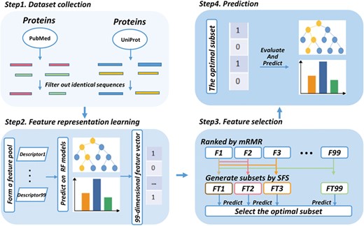
Framework of the proposed QSPred-FL. Firstly, query proteins are scanned by a window with the predefined length to generate peptide sequences, among which the identical sequences will be subsequently filtered out. Secondly, the resulting peptide sequences are subjected to the feature representation learning scheme, and as a result, a 99-dimensional feature vector will be generated. Thirdly, the feature vector generated at the previous step is optimized to a 4-dimensional optimal feature vector using a two-step feature selection strategy. Ultimately, the peptides are predicted and scored by the well-trained RF model.
RF
In this work, we employed the RF [21] algorithm to build models and make predictions. RF has been widely used in bioinformatics and computational biology [22–30]. For implementation, we used the RF algorithm embedded in a data mining tool called WEKA (Waikato Environment for Knowledge Analysis) [31]. All the experiments in this paper were done under version 3.8 of WEKA with default parameters (tree number = 100).
Feature representation
AAC
CTD
This feature-encoding algorithm combines three descriptors: composition (C), transition (T) and distribution (D). The composition descriptor is used to classify all amino acids into three categories and calculate the percent of each category as features for a particular physicochemical property in the peptide sequence. The three features of the transition descriptor for a particular property are the frequencies of three kinds of residue pairs, for which two adjacent residues are (1) a negative residue followed by a neutral one, (2) a positive residue followed by a negative one and (3) a positive residue followed by a neutral one, respectively. The distribution descriptor describes the fractions of the entire peptide sequence where the first, 25, 50, 75 and 100% of amino acids of a particular property are placed within the peptide sequence, respectively [34, 35]. By concatenating the three feature descriptors, we yielded a 63-dimensional vector for the CTD descriptor [35].
188-bit features
This descriptor is a combination of AAC and the extension of CTD, measuring AAC and physicochemical information. In this descriptor, there are a total of 188 features. The first 20 features are the occurrence frequencies of 20 different amino acids extracted from AAC. The other 168 features are obtained from the extension of CTD, for which a total of eight physicochemical properties are considered, including surface tension, hydrophobicity, solvent accessibility, normalized Van der Waals volume, polarity, polarizability, secondary structures and charge [35–37]. For each property, 20 different amino acids are classified into three groups. The classification information of each property can be found in Table S1 (Supporting Information). Therefore, using the extension of the CTD, we obtained 168 features for all eight physicochemical properties.
GDC
ASDC
IT
N- and C-terminus approach
Some specific residues, like Ala, Pro and Lys, are found to prefer the location at N- and C-terminus (NT-CT) of peptides, indicating that features in local subsequences might be more informative than that based on the full-length peptides. Therefore, we introduce a NT-CT approach to extract subsequences with a certain length from the N- or C-terminus of a given peptide. Here we extracted a fixed-length sub-sequence from the peptide in three ways: N- terminus, C-terminus and both N- and C-terminus, respectively [41]. The three approaches are termed as NT, CT and NT-CT. The sequence length by the above three approaches are |$t$|, |$t$| and 20 × |$t$|, where |$t$|denotes the length of N- or C-terminus.
BPF
21-bit features
The 21-bit method takes seven important physicochemical properties of the amino acid sequences into consideration: hydrophobicity, solvent accessibility, normalized Van der Waals volume, polarity, polarizability, secondary structures and charge [35]. The standard amino acid alphabet is divided into three groups based on each property and encoded with 0 or 1 according to their groups, where 1 denotes that the amino acid belongs to the group and 0 denotes not [38]. The details of the groups corresponding to each physicochemical property can be found in Table S2 (Supporting Information). Thus, the peptide is encoded by the descriptor into a 21-dimensional 0/1 feature vector.
OVP
The 20 amino acid types are classified into 10 groups according to 10 physicochemical properties [42]. The details of the 10 groups are provided in Table S3 (Supporting Information). For each property, if its residue of one peptide belongs to the group, the parameter will be set to 1 and 0 otherwise. For a given peptide, it is represented as a 10-dimensional vector using this descriptor.
Feature representation learning scheme
In our previous study [38], we proposed a feature representation learning scheme, showing the effectiveness for extracting the informative features from existing feature descriptors. Here, we upgraded this scheme by integrating more different types of sequence-based feature descriptors. The upgraded version of the feature representation learning scheme is composed of the following three steps, as illustrated in Figure 2.
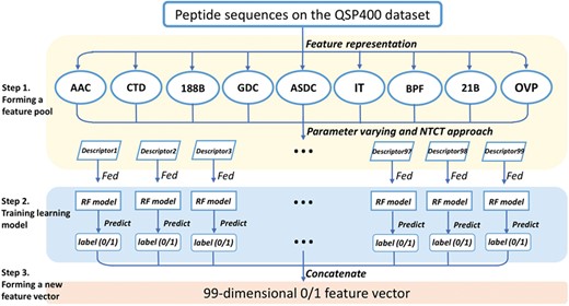
Pipeline of the feature representation learning scheme. Firstly, a feature pool with 99 feature descriptors is constructed by nine feature-encoding algorithms and the NT-CT approach. Afterwards, each descriptor is trained and evaluated using the RF classifier on the QSP400 dataset. Finally, the predicted class label for each trained RF model is regarded as an attribute to form a new feature vector.
Step 1. Forming a feature pool
We have utilized nine feature extraction methods for feature representation, including AAC, CTD, 188-bit, GDC, ASDC, IT, BPF, 21-bit and OVP. To make our feature extraction methods diverse, effective and discriminative, we set the method parameter |$k$| to 1 or 2 in AAC and the gap parameter |$g$| from 1 to 4 in GDC. Meanwhile, we utilize the three approaches, NT, CT and NT-CT, to combine with several aforementioned methods, AAC, BPF, 21-bit features, ASDC, OVP and IT. In the QSP400 dataset, the minimal length of the peptide sequences is five residues. Thus, the parameter|$t$| used in the NT-CT approach ranges from 1 to 5. To this end, we yielded 99 feature descriptors in total. The list of all the 99 descriptors are provided in Table S4 (Supporting Information).
Step 2. Training learning model
For the 99 feature descriptors, each was trained with the RF classifier on the QSP400 dataset, and then, was evaluated with 10-fold cross validation. If the predicted class label is assigned as 0, which indicates the given peptides are predicted to be QSPs, and as 1 otherwise.
Step 3. Forming a new feature vector
The predicted class labels obtained from each descriptor are regarded as a new attribute to form a new feature vector. The dimension of the new feature vector is 99.
Feature selection
Feature selection is a key step for building a powerful machine learning model [43–57]. In order to improve the ability of feature representation, we used a two-step feature selection strategy to extract the most discriminative features [23, 38, 42, 58–62]. The process of this strategy is described below. The first step is to rank the 99 feature descriptors based on their classification importance by mRMR [14]. The higher rank the descriptor gets, the more important the feature is. The second step is to determine the optimal feature subset by the SFS strategy [16]. The SFS strategy constructs a feature subset by adding the feature one by one from the ranked features and trains the RF model with the respective feature subset. The models are subsequently evaluated by 10-fold cross validation. The feature subset, corresponding to the RF model with the highest accuracy, is considered as the most discriminative features to distinguish true QSPs from non-QSPs. The determination of the optimal features is discussed in `Results and Discussion’.
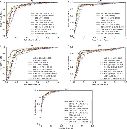
ROC curves of the top 10 best-performing feature descriptors using five different classifiers. (A)–(E) represent the ROC curves of NB, SVM, LR, J48 and RF, respectively.
Performance measurements
Receiver operating characteristic curve
To intuitively evaluate the overall performance, we employed the receiver operating characteristic (ROC) curve in this study. It is plotted by calculating sensitivity (True Positive Rate; TPR) against 1-specificity (False Positive Rate; FPR) under different thresholds [64–66]. The area under the ROC curve, termed as AUC, is often used as a metric to access the overall performance. The AUC score ranges from 0.5 to 1. The larger score a predictor achieves, the better performance it has.
Ten-fold cross validation
Here, the 10-fold cross validation method is used as the performance evaluation method [67–78]. The procedure is described as follows. For a given dataset, it is firstly divided into 10 subsets randomly, for which one single subset is used as the validation dataset and the remaining nine as the training dataset. Secondly, the model is trained with the training dataset and evaluated by the validation dataset. The procedure is repeated until each subset serves as the validation dataset. Ultimately, the performance of a predictor is yielded by averaging the performance on the 10 subsets.
Results and discussion
Comparative analysis of feature descriptors using different classifiers
As described in section `Feature representation’, we reviewed nine different types of sequence-based feature representation encoding algorithms. By varying the feature parameters, we yielded a total of 99 feature descriptors as described in section `Feature representation learning scheme’ (see Table S4 in Supporting Information). To conduct a comprehensive comparison analysis, we compared all the 99 feature descriptors using different classifiers. For this purpose, we employed five commonly used classifiers: RF, Naïve Bayes (NB), SVM, Logistic Regression (LR) and J48, respectively. For each classifier, we trained the classifier with all the feature descriptors, respectively, and evaluated the trained classifiers on the same dataset with the 10-fold cross validation. Therefore, we yielded a total of 495(= 99 * 5) predictive models for the 99 feature descriptors and five classifiers. The results for all the feature descriptors under the five classifiers are summarized in Tables S5–S9 (see Supporting Information), respectively.
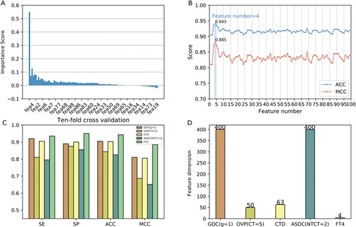
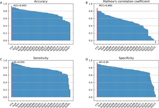
The results of feature selection. (A) The importance scores of the sorted features. (B) The performances of feature subsets using SFS in terms of ACC and MCC. (C) The performance of the optimal features (FT4) and the original four feature descriptors in terms of SE, SP, ACC and MCC. (D) The feature number of the optimal features (FT4) and the original four feature descriptors.
From Tables S5–S9, we observed that different feature descriptors achieved the best overall predictive performance using different classifiers. For example, using the NB classifier, the GDC (g=4) achieved the highest ACC of 88.8% and MCC of 0.775 among the 99 feature descriptors (Table S5), 2% and 4% than that of the second best GDC (g=3) descriptor, respectively. Among the feature descriptors trained with the SVM classifier, the AAC (k=2) obtained the best performances, giving the maximal ACC of 92.3% and MCC of 0.845. Likewise, as for the feature descriptors based on the LR classifier, the AAC (k=2) achieved the best as well. Moreover, the 188-bit outperforms the other feature descriptors with higher ACC and MCC for the remaining classifiers LR and RF. These results demonstrate that the performance of existing feature descriptors is greatly impacted by the used classifiers. Not any feature descriptor can exhibit the superior performance. Next, we further compared the best feature descriptors regarding the five classifiers. We can see that the AAC (k=2) coupled with the SVM classifier is significantly better than the other four combinations, 1.8–6% and 3.5–11% higher in terms of ACC and MCC, respectively (Tables S5–S9). In other words, this combination is the best among all the 495 combinations of features and classifiers. In general, by comprehensively analyzing all the feature descriptors with different kinds of classifiers, it can be concluded that the SVM classifier trained with the AAC (k=2) descriptor has more discriminative power to classify true QSPs from non-QSPs.
In addition, we also investigated which classifiers are more effective for the prediction of QSPs. For more intuitive comparison, we plotted the ROC curves of the top 10 best feature descriptors of each classifier and calculated their corresponding AUC scores as illustrated in Figure 3. We observed that the AUCs of the feature descriptors using the RF classifier are generally higher than that using the other classifiers. This demonstrates that the RF has stronger power than the other four classifiers. As for the other classifiers, the SVM, NB and LR are competitive with each other, while the performance of J48 classifier is the worst among the five compared classifiers in terms of AUC.
Performance of the optimal feature descriptor and the 99 feature descriptors. (A)–(D) plot the performances in terms of ACC, MCC, SE and SP, respectively. Note that FT4 represents the optimal 4-dimenisonal feature vector.
Feature representation learning and selection analysis
In this work, we employed a two-step feature selection strategy to select the optimal feature subset from the 99 learnt features. In this strategy, we firstly ranked all the features based on their classification importance by mRMR. The sorted features with their corresponding importance scores are shown in Figure 4A. The importance scores of features are listed in Table S10 (Supporting Information). As can be seen, the fourth feature among the 99 features is the most important for classification, with an importance score of 0.55. Afterwards, we added the feature one by one from the ranked features and trained the added features. The overall performances in terms of ACC and MCC of feature selection using the SFS are depicted in Figure 4B. More detailed results are summarized in Table S11 (see Supporting Information). As we can see in Figure 4B, the performance increases rapidly with the features increasing. When the number of features increases to 4, the predictive performance achieved the peak, with the highest ACC of 94.3% and MCC of 0.885, respectively. After that, the performances drop significantly as the feature number increases, and finally stabilize at the ACC and MCC of about 92% and 0.83, respectively. Consequently, we used the first four features of the ranked features as our optimal feature subset. It should be noted that the four features in the optimal feature subset is generated from four descriptors in our proposed feature representation learning system: GDC (g = 1), OVP (CT = 5), CTD and ASDC (NTCT = 2), respectively.
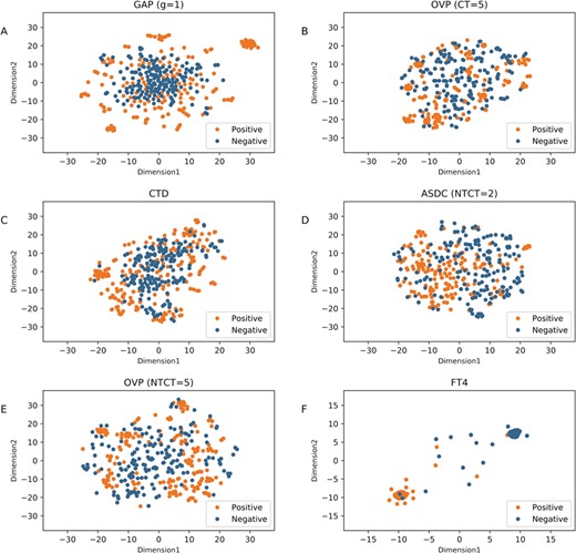
t-SNE distribution of positive and negative samples in the dataset using our optimal descriptor and these five individual descriptors. (A)–(F) are the distribution of GDC (g = 1), OVP (CT = 5), CTD, ASDC (NTCT = 2), OVP (NTCT = 5) and FT4 (our optimal descriptor), respectively.
Next, we further compared the performance of the optimal feature vector with that of the original four descriptors. The performance evaluations of the four descriptors and the optimal feature descriptor on the QSP400 dataset with 10-fold cross validation are shown in Figure 4D. The results of all the 99 individual feature descriptors can be found in Table S9 (Supporting Information). As we can see, our optimal feature descriptor exhibits better performance in terms of all the metrics: ACC, SE, SP and MCC, as compared to the other four feature descriptors. Specifically, the optimal descriptor achieved a maximal ACC of 94.3% and MCC of 0.885, significantly higher than GDC (g = 1) (ACC = 90.5% and MCC = 0.81), OVP (CT = 5) (ACC = 84.3% and MCC = 0.686), CTD (ACC = 90.3% and MCC = 0.805), ASDC (NTCT = 2) (ACC = 82.5% and MCC = 0.651), respectively. This indicates that the optimal features are more accurately to distinguish true QSPs from non-QSPs than its original feature descriptors. Importantly, the dimension of our optimal feature vector is 4, far fewer than the four feature descriptors (Table S4 and Figure 4C). Moreover, it is also interesting to further see whether the optimal feature descriptor outperforms all the 99 feature descriptors in the feature representation learning scheme. The performance of our optimal feature descriptor and all the feature descriptors are illustrated in Figure 5. We can see from Figure 5 that in comparison with the other feature descriptors, the learnt 4-dimensional feature vector achieved significantly better performance in terms of three out of the four major metrics: SP, MCC and ACC, with the only exception of SE.
Ten-fold cross validation performance of the RF classifier and other four classifiers on the QSP400 dataset
| Classifiers | SE (%) | SP (%) | ACC (%) | MCC | TP | TN | FP | FN |
|---|---|---|---|---|---|---|---|---|
| NB | 87.0 | 88.5 | 87.75 | 0.755 | 174 | 177 | 26 | 23 |
| SVM | 90.0 | 92.5 | 91.25 | 0.825 | 180 | 185 | 20 | 15 |
| LR | 86.5 | 87.5 | 87.0 | 0.740 | 173 | 175 | 27 | 25 |
| J48 | 89.0 | 81.5 | 85.25 | 0.707 | 178 | 163 | 22 | 37 |
| RF | 93.5 | 95.0 | 94.3 | 0.885 | 187 | 190 | 10 | 13 |
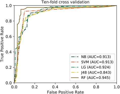
ROC curves of the RF classifier and other four classifiers on the QSP400 dataset.
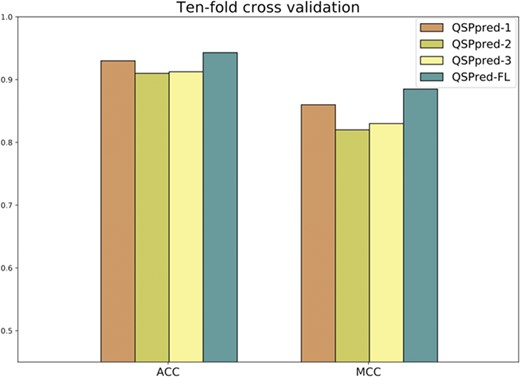
Performance comparison of the proposed predictor QSPred-FL and the three other predictive models of QSPpred with 10-fold cross validation on the QSP400 dataset.
To analyze why our features are more effective than the individual feature descriptors, we plotted the t-Distributed Stochastic Neighbor Embedding (t-SNE) distribution of positive and negatives in the dataset using the optimal descriptor and the top five individual descriptors ranked by mRMR in the two-dimensional feature space, which are illustrated in Figure 6. As shown in Figure 6, we can clearly see that for the original five feature descriptors (Figure 6A–E), the positives and negatives are mixed up in feature space. In contrast, in our optimal feature space, we can see that most of positives and negatives are distributed in two clusters (Figure 6F), while only a few points (samples) are mixed. These results suggest that the true QSPs (positives) and non-QSPs (negatives) in our feature space can be easier to be discriminated as compared to that in the other feature space, thereby improving the performance. On the other hand, this also indicates that our feature representation learning scheme can provide an effective way to improve the predictive performance. In general, this scheme has the following three advantages: (1) it is completely parameter-free; in this scheme, we do not need to tune the parameters for specific datasets as most of the existing feature descriptors do. (2) It can effectively transform the high-dimensional feature space into low-dimensional feature space, thus speeding up the prediction process and explore the application of our predictor in genome-wide prediction. (3) More importantly, the feature representation learning and selection scheme are scalable, not only for peptide feature representation but also for protein feature representation.
Classifier comparative analysis based on the optimal features
In this study, we used the RF classifier to establish the predictive model. To investigate the impact of other machine learning algorithms for the performance, we compared the RF classifier with other four commonly used classifiers, including NB, SVM, Logistic LR and J48. For fair comparison, we trained different classifiers with the same feature vector we yielded (4-dimensional feature vector) on the QSP400 dataset. It should be mentioned that all the compared machine learning algorithms were tuned to the best in this study. Table 1 provides the 10-fold cross evaluation performance of the RF and other four classifiers on the QSP400 dataset, and Figure 7 depicts their corresponding ROC curves.
As shown in Table 1, the RF classifier achieved significantly better overall performance with an ACC of 94.3% and MCC of 0.885 as compared to the other classifiers. To be specific, the performances of RF in terms of ACC and MCC are 2.15% and 0.06 higher than the second-best classifier compared SVM with the ACC of 91.25% and MCC of 0.825, respectively. Additionally, the RF achieved an SE of 93.5% and SP of 95%, which are 3.5–7% and 2.5–13.5% higher than the other four classifiers, respectively. As for the ROC curves in Figure 7, the RF obtained an AUC of 0.945, remarkably outperforms NB (AUC = 0.913), SVM (AUC = 0.913), LR (AUC = 0.924) and J48 (AUC = 0.843). These results demonstrate that the RF classifier has better predictive power in comparison with other classifiers.
Comparison with the state-of-the-art predictors
To evaluate the effectiveness of our proposed predictor, we evaluated and compared our predictor with the state-of-the-art predictor QSPpred, only one available predictor in the literature [17]. Since there are several predictive models using different feature descriptors in QSPpred, we chose the top three predictive models of QSPpred for comparisons. The features used in the three models are Physico, AAC + DPC + N5C5Bin and AAC + DPC + N5C5Bin + Physico, respectively, where Physico represents Physicochemical features; AAC denotes Amino Acid Composition; DPC denotes Dipeptide composition; N5C5Bin denotes Binary profile features of N5C5 terminus. For convenience of discussion, they are denoted as QSPpred-1, QSPpred-2 and QSPpred-3, respectively.
The 10-fold cross validation results of QSPred-FL and the three predictive models of QSPpred on the QSP400 dataset are depicted in Figure 8, where we can observe the following two aspects. Firstly, as for the three predictive models of QSPpred, the QSPpred-1 model outperforms the other two models in terms of ACC and MCC, achieving an ACC of 93% and an MCC of 0.86. Secondly, our predictor reached the highest ACC of 94.3% and MCC of 0.885, which are 1.3% and 2.5% higher than that of the second-best predictor QSPpred-1. This suggests that our predictor can more effectively classify true QSPs from non-QSPs than the existing predictors. More importantly, our predictor uses only four features in our predictive model, far fewer than the predictive models of the QSPpred, showing the potential to become an efficient predictor for the large-scale identification of QSPs.
Webserver implementation
In order to facilitate researchers’ effects to identify putative QSPs, we have established a user-friendly webserver that implements the proposed predictor, which is freely accessed via http://server.malab.cn/QSPred-FL. Below, we give researchers a step-by-step guideline on how to use the webserver to get their desired results. In the first step, users need to submit the query sequences into the input box. Note that the input sequences should be in the FASTA format. Examples of the FASTA-formatted sequences can be seen by clicking on the button FASTA format above the input box. Next, users need to set the prediction parameters before running predictions. Here, the parameter is the prediction confidence, ranging from 0.5 to 1. The higher confidence users set, the more sensitive predictions users get. Finally, clicking on the button Submit, you will get the predicted results.
Conclusion
In this study, we have conducted a comprehensive and comparative study of 99 feature descriptors (included in nine different sequence-based feature-encoding algorithms with different parameters) using five different machine learning algorithms for the computational identification of QSPs. Our findings demonstrated that the predictive model trained with the AAC features (k = 2) and the SVM classifier could lead to the best predictive performance among the compared 495 machine learning models. To build a high efficient and accurate prediction model, we have established a feature representation learning and feature selection scheme to extract the most discriminative features. Our results indicate that the proposed scheme can effectively improve the predictive performance for the prediction of QSPs as compared to existing sequence-feature descriptors. Therefore, this scheme can provide a new and useful strategy regarding how to more effectively and efficiently extract discriminative features from the existing feature descriptors. Using the learnt informative features, we further developed a RF-based predictor, namely QSPred-FL. We have benchmarked this proposed predictor with the state-of-the-art predictor QSPpred. The results have shown that using much fewer features, QSPred-FL is able to achieve more effective and accurate performance in QSP prediction. We anticipate that QSPred-FL will be a powerful bioinformatics tool for accelerating the discovery of novel putative QSPs and can be used to provide insights into the functional mechanisms of QSPs. In future work, integrating motif analysis for the predictions generated from our predictive model is expected to decrease the false positives, therefore reducing the cost of post-experimental validation for biological researchers [79–82].
We comprehensively analyze a variety of existing sequence-based feature descriptors and machine learning algorithms for the prediction of QSPs.
We introduce a feature representation learning algorithm, QSPred-FL, that enables the learning of informative features from several high-dimensional feature space.
QSPred-FL integrates the class information from a total of 99 random forest models trained based on multiple sequence-based feature-encoding algorithms.
Comparative studies showed that QSPred-FL outperforms a number of currently available predictors. It is publicly accessible at http://server.malab.cn/QSPred-FL.
Funding
The National Key R&D Program of China (SQ2018YFC090002), the National Natural Science Foundation of China (61701340, 61702361 and 61771331), the Australian Research Council (LP110200333 and DP120104460), the National Health and Medical Research Council of Australia (NHMRC) (4909809), the National Institute of Allergy and Infectious Diseases of the National Institutes of Health (R01 AI111965), a major inter- disciplinary research project awarded by Monash University and the collaborative research program of the Institute for Chemical Research, Kyoto University (2018–28).
Leyi Wei received his PhD degree in Computer Science from Xiamen University, China. He is currently an assistant professor at the School of Computer Science and Technology, Tianjin University, China. His research interests include machine learning and their applications to bioinformatics.
Jie Hu received her BSc degree in Resource Environment and Urban Planning Management from Wuhan University of Science and Technology, China. She is currently a graduate student at the School of Computer Science and Technology, Tianjin University, China. Her research interests are bioinformatics and machine learning.
Fuyi Li received his BEng and MEng degrees in Software Engineering from Northwest A&F University, China. He is currently a PhD candidate at the Department of Biochemistry and Molecular Biology and the Infection and Immunity Program, Biomedicine Discovery Institute, Monash University, Australia. His research interests are bioinformatics, computational biology, machine learning and data mining.
Jiangning Song is a senior research fellow and group leader at the Biomedicine Discovery Institute and Department of Biochemistry and Molecular Biology, Monash University, Melbourne, Australia. He is a member of the Monash Centre for Data Science and an associate investigator of the ARC Centre of Excellence in Advanced Molecular Imaging, Monash University. His research interests primarily focus on bioinformatics, computational biology, machine learning and pattern recognition.
Ran Su is currently an associate professor at the School of Computer Software, Tianjin University, China. Her research interests include pattern recognition, machine learning and bioinformatics.
Quan Zou is a professor of Computer Science at Tianjin University and the University of Electronic Science and Technology of China. He received his PhD in Computer Science from Harbin Institute of Technology, P.R. China in 2009. His research is in the areas of bioinformatics, machine learning and parallel computing, with focus on genome assembly, annotation and functional analysis from the next generation sequencing data with parallel computing methods.
References
