


Abstract
Cancer is a collection of genetic diseases, with large phenotypic differences and genetic heterogeneity between different types of cancers and even within the same cancer type. Recent advances in genome-wide profiling provide an opportunity to investigate global molecular changes during the development and progression of cancer. Meanwhile, numerous statistical and machine learning algorithms have been designed for the processing and interpretation of high-throughput molecular data. Molecular subtyping studies have allowed the allocation of cancer into homogeneous groups that are considered to harbor similar molecular and clinical characteristics. Furthermore, this has helped researchers to identify both actionable targets for drug design as well as biomarkers for response prediction. In this review, we introduce five frequently applied techniques for generating molecular data, which are microarray, RNA sequencing, quantitative polymerase chain reaction, NanoString and tissue microarray. Commonly used molecular data for cancer subtyping and clinical applications are discussed. Next, we summarize a workflow for molecular subtyping of cancer, including data preprocessing, cluster analysis, supervised classification and subtype characterizations. Finally, we identify and describe four major challenges in the molecular subtyping of cancer that may preclude clinical implementation. We suggest that standardized methods should be established to help identify intrinsic subgroup signatures and build robust classifiers that pave the way toward stratified treatment of cancer patients.
Introduction
Cancer is a large group of genetic diseases that are currently classified by their primary site of origin, such as brain cancer, breast cancer and lung cancer. However, not all cancers of an organ are the same, and genetic heterogeneity exists between and within cancers [1–6]. A major cause of this heterogeneity is genomic instability [7] that can act at the single-nucleotide level, or at much larger scales [8]. This poses significant challenges to the efficacy of currently applicable targeted therapies and complicate the development of future treatment strategies [7]. Because of this, there is a great need to classify cancer into homogeneous groups that associate with distinct molecular features and clinical outcomes and allow the development of subgroup specific therapies.
The traditional classification of cancer has been carried out by pathologists based on histological appearance and site of growth. This only partially reflects the true heterogenic character of cancer. Recent advances in genome-wide profiling techniques [9, 10] have allowed researchers to generate large-scale genomic data and classify cancer into more homogeneous groups [11, 12]. Genomic data have been used in many cancer subtyping studies, including leukemia [13], lymphoma [14], nasopharyngeal carcinoma (NPC) [15], breast [16], lung [17], liver [18], pancreas [19], colon [20] and soft tissue sarcomas [21]. Various machine learning algorithms [22–26] have also been developed for better prediction of cancer subtypes. Molecular subtyping studies have allowed the classification of cancer into uniform groups that correlated better with clinical outcomes than the traditional classifications of cancer [27]. In summary, the molecular classification can provide diagnostic, prognostic and therapeutic options for the treatment of cancers.
This review is organized as follows: in ‘Molecular subtyping of cancer’ section, we first introduce two techniques that are used for cancer subtyping: microarray and RNA sequencing (RNA-Seq). Next, we introduce three other frequently applied techniques for generating low- and medium-throughput molecular data; quantitative polymerase chain reaction (qPCR), NanoString and tissue microarray (TMA), and we discuss their applications in clinical tests. Subtype identifications and characterizations, which are the two important aspects involved in the subtyping process are also discussed. In ‘Moving toward clinical applications’ section, we illustrate potential clinical applications of cancer subtyping studies for diagnosis, prognosis, predicting therapy response and drug design. In ‘Challenges’ section, we identify and describe four major challenges in the molecular subtyping of cancer that may preclude clinical implementation, and finally, in ‘Conclusions and outlook’ section, we provide the concluding remarks and recommendations.
Molecular subtyping of cancer
Recent advances in genome-wide profiling techniques have allowed the generation of large-scale genomic data, and various statistical and machine learning algorithms have been developed for processing and interpretation of such data [23–25, 28–31]. Molecular subtyping of cancer, as its name suggests, is a new way to classify cancers into different groups based on molecular data and classification models. Contrary to the traditional histological classification of cancer, molecular classifications rely on biomarkers and classifiers. Biomarkers can be informative genes, microRNAs (miRNAs), DNA methylation markers and others [32]. Classifiers can be built by machine learning algorithms, such as Prediction Analysis for Microarrays (PAM), Support Vector Machines (SVMs) and more [33]. In the following, we will provide an introduction of different molecular data types and their applications, to a workflow for unsupervised classification of cancer.
High-throughput molecular data for cancer subtyping
Gene expression profiling data for cancer subtyping
Microarray and RNA-Seq are two common profiling techniques for generating high-throughput gene expression data. Microarrays are capable of profiling expression patterns for tens of thousands of selected genes in a single assay [9]. RNA-Seq is a sequencing-based method to determine the amount of gene abundance from the entire genome. There are numerous advantages of RNA-Seq over microarray [34]. First, unlike hybridization-based microarrays, RNA-Seq provides more accurate detection of gene expression. Second, RNA-Seq can detect novel transcripts, single-nucleotide variants and other (yet) unknown changes that microarray cannot detect. Finally, RNA-Seq has low background signal, and consequently has a large dynamic range. Microarray has been the most commonly used technique to generate large-scale molecular data for several decades [35]. With the fast development of sequencing and analyzing techniques, the sequencing cost will dramatically decrease and more statistical tools will be developed for RNA-Seq, and RNA-Seq will likely replace microarray [36]. Compared with other molecular profiling techniques, microarray and RNA-Seq are the most accurate, reliable and robust, but are also expensive, time-consuming and sample quality-dependent techniques (Table 1). They are commonly used in the initial biomarkers identification process. If biomarkers have been identified, other techniques are preferred.
A comparison of different techniques for molecular profiling of cancer
| Platform | |||||
|---|---|---|---|---|---|
| Characteristic | Microarray | RNA sequencing | qPCR | NanoString | Tissue microarray |
| Accuracy [37, 166, 167] | Median | Median | High | High | Low |
| Sensitivity [36, 167, 39] | Median | High | High | High | Low |
| Specificity [38, 167, 168] | Median | Median | High | High | Low |
| Speed [36, 167] | Slow | Slow | Fast | Median | Slow |
| Cost (per sample) | $300 [163] | $1000 [163] | $280 [164] | $800 [39] | $100 [165] |
| Sample requirement [167] | FFPE/fresh-frozen | FFPE/fresh-frozen | Fresh-frozen | FFPE/fresh-frozen | FFPE |
| Genome-wide coverage | Yes | Yes | No | No | No |
| Quantitative | Yes | Yes | Yes | Yes | No |
| Single-base resolution | No | Yes | No | No | No |
| Low sample input | No | No | Yes | No | Yes |
| Reproducibility [168] | Median | Median | High | High | Low |
Gene expression-based subtyping of cancer was first proposed by Golub et al. [13] in leukemia. The expression pattern of the 50 most informative genes was measured and a two-cluster self-organizing map (SOM) clustering method was applied [40] to group 38 samples into two classes: acute myeloid leukemia and acute lymphoblastic leukemia with accuracy of 100%. This demonstrated the fidelity of cancer subtyping based solely on gene expression patterns [13]. Gene expression-based subtyping now has been extended to include many cancer types [11, 14, 16, 17, 19, 21, 41].
Multi-platform profiling data for cancer subtyping
In addition to gene expression profiling, there are many other molecular profiling data types, such as mutation, miRNA expression, copy number variation (CNV) and DNA methylation, which can be used to identify and characterize cancer subtypes (Table 2) [43, 44, 50, 52–55]. As all cancers arise as a result of DNA sequence changes [56], the gene mutation patterns are informative and a likely platform from which to stratify cancer patients into homogeneous groups [57, 58]. MiRNAs are small noncoding RNAs about 20–22 nucleotides in length that play key roles in the regulation of gene expression. Alterations of miRNA expression are involved in the initiation and progression of human cancer [59–61]. MiRNA expression profiling now has been used as a new tool in cancer onset and subtyping [15, 62]. Unlike mRNAs, miRNAs are more stable and only a small number of miRNAs (∼200 in total) are sufficient to classify human cancers [63]. CNVs are structural variations and genomic alterations that affect DNA sequence lengths ranging from approximately 1 Kb to 3 Mb [64]. CNVs are associated with many complex diseases such as neuropsychiatric disorders [65], HIV [66], familiar pancreatitis [67] and cancers [68, 69]. Comparative genomic hybridization (CGH) can be used to detect CNVs at the genome-wide level, and array-based CGH can increase the resolution for better genomic studies. Epigenetic changes such as DNA methylation also play a significant role in the development and progression of cancer [70]. Bisulfite sequencing [71] and differential methylation hybridization [72] can be used to scan gene methylation status at the genome-wide level.
Molecular subtyping studies mentioned in the review
| Cancer type | Discovery sample size | Molecular data type | Clustering method | Determinative score | Number of subtypes | Classification method | Reference |
|---|---|---|---|---|---|---|---|
| Breast cancer | 65 | mRNA | Hierarchical clustering | NA | 4 | NA | Perou et al .[16] |
| Breast cancer | 85 | mRNA | Hierarchical clustering | NA | 5 | NA | Sorlie et al. [42] |
| Breast cancer | 825 | Five platforms | Cluster of clusters | NA | 4 | NA | TCGA [43] |
| Breast cancer | 2, 000 | mRNA + CNV | iCluster | ARI | 10 | PAM | Curtis et al. [44] |
| CRC | 62 | mRNA | Iterative NMF | Cophenetic coefficient | 5 | NA | Schlicker et al. [45] |
| CRC | 443 | mRNA | Orig. cons. clustering | CDF area | 6 | Centroid-based | Marisa et al. [46] |
| CRC | 90 | mRNA | Orig. cons. clustering | Gap statistic | 3 | PAM | De Sousa E Melo et al. [20] |
| CRC | 445 | mRNA | NMF cons. clustering | Cophenetic coefficient | 5 | PAM | Sadanandam et al. [47] |
| CRC | 1, 113 | mRNA | Orig. cons. clustering | Dynamic cut tree | 5 | Multiclass LDA | Budinska et al. [48] |
| CRC | 188 | mRNA | k-means | NA | 3 | Single-sample centroid based | Roepman et al. [49] |
| CRC | 4, 151 | mRNA | Markov Cluster Algorithm | Inflation factor | 4 | Random Forest | Guinney et al. [11] |
| PDAC | 185 | miRNA | Hierarchical clustering | CDF area | 2 | SVM | Bauer et al. [50] |
| PDAC | 66 | mRNA | NMF cons. clustering | Cophenetic coefficient | 3 | NTP | Collisson et al. [19] |
| PDAC | 223 | mRNA | NMF cons. clustering | Cophenetic coefficient | 2 | Rank-based classifier | Moffitt et al. [51] |
| Pancreatic cancer | 96 | mRNA | NMF cons. clustering | Cophenetic coefficient | 4 | NA | Bailey et al. [12] |
| Leukemia | 38 | mRNA | SOM | NA | 2 | NA | Golub et al. [13] |
| Leukemia | 200 | Methylation | PCA | NA | 16 | NA | Figueroa et al. [169] |
| Lymphoma | 42 | mRNA | Hierarchical clustering | NA | 2 | NA | Alizadeh et al. [14] |
| GBM | 35 | miRNA | PCA | Ratio of intracluster to intercluster correlation | 2 | LDA | Marziali et al. [170] |
| Lung | 67 | mRNA | Hierarchical clustering | NA | 4 | NA | Garber et al [17] |
| 12 cancer types | 3, 527 | Five platforms | COCA | NA | 11 | NA | Hoadley et al [32] |
Note: ARI, adjusted Rand index; No., number; COCA, Cluster-Of-Cluster-Assignments; iCluster, integrative clustering framework; LDA, linear discriminant analysis; NTP, nearest template prediction; Orig. cons., original consensus; PCA, principal component analysis.
Integrating the analysis of multiple genomic data, such as gene expression with CNV [44], miRNA with gene expression [73] and five-platform combined subtyping [32] studies can provide even better insights into tumor biology, and more accurate predictions, than the analysis at a single molecular level [74]. With the advances in high-throughput profiling technologies, the expenses spent on each sample are decreasing; thus, multi-platform identification and characterization of cancer is likely to become the norm.
Low- and medium-throughput molecular data for clinical test
Biomarkers identified from subtyping studies can be used in clinical practice. In typical clinical settings, only up to several dozens of these predefined biomarkers are measured to minimize the time and expenses spent on the tests [75]. In addition, most cancer specimens are formalin-fixed paraffin-embedded (FFPE), and only few are freshly prepared or snap frozen [76]. In contrast to the above mentioned high-throughput approaches, some low- and medium-throughput profiling techniques (such as qPCR, NanoString and TMA) that allow meaningful analysis of clinical specimens are well suited for clinical use of biomarker assays. These techniques are frequently used when fast detection time is required, and sample volume and pricing should be kept low. Sensitivity and specificity are the two terms used to evaluate a clinical test. Sensitivity refers to the ability of a test to correctly identify an individual with disease; specificity refers to the ability of a test to correctly identify an individual without the disease [77]. Another important term in the evaluation of a clinical test is to determine its accuracy, which describes the errors that a test will produce when differentiating between individuals with and without the disease [78]. In the following, we will compare these three techniques (qPCR, NanoString and TMA) in terms of accuracy, sensitivity, specificity and other aspects of concerns involved in a clinical test. Researchers can choose appropriate techniques for their clinical assays based on the comparisons provided in Table 1.
qPCR is commonly used to determine biomarker expression levels, or to assess CNVs. Because there is a PCR amplification step, which can greatly increase the nucleic acid input, only limited sample quantity is needed. Other advantages of qPCR include fast, high sensitivity, specificity and accuracy, which make it the routine method for validation of results initially obtained from high-throughput methods such as microarray and RNA-Seq [79]. Compared with other techniques, which can assay hundreds to thousands biomarkers, qPCR-based assays can only handle a limited number of biomarkers in a single test. qPCR-based tests also require high quality of the nucleic acids in the sampled material, so fresh-frozen tissues are typically required for qPCR.
The NanoString nCounter analysis system can be used to measure expression levels of up to 800 genes [80]. Developed by Geiss et al. [39], the nCounter system is more sensitive than microarrays, and similar in sensitivity to qPCR [39]. This technology uses digital molecular barcoding and microscopic imaging to detect and quantify the expression levels of genes in a single assay without enzymatic reactions [39, 81]. Other advantages of this technique include high accuracy and specificity [38]. Disadvantages include the high cost of the required reagents and instruments [80].
TMA is a histology-based test, developed by Kononen et al. [82], which allows the analysis of up to 1000 tumor specimens simultaneously in a single paraffin block [37]. Analysis of molecular targets at the DNA, mRNA and protein levels is possible. Once constructed, a TMA block can be sectioned hundreds of times (provided the depth of all cores is sufficient), with each section amenable to biomarker analysis. The most significant advantage of TMA is that all samples on the array are treated in an identical fashion [83]. Another advantage of TMA is that it is cost-effective (Table 1). Only a small amount of reagent is required to analyze all the samples on one slide [83]. Unlike qPCR, which requires fresh-frozen tissues, TMA requires FFPE tissues, which are the major source of material in the clinic. TMA also has limitations. For instance, low sensitivity, specificity and accuracy are the typical features of a TMA test [84]. Other disadvantages include: it usually takes several days to obtain the analysis results [85], only a limited number of analytes can be tested and the analyzed specimen volume is too small to represent the entire tumor [83]. Also during the TMA staining process, the amount of tissues will become less and less [86].
Subtype identifications and characterizations
Molecular subtyping (or molecular classification) is a process of assigning data objects into clusters, so that objects in the same cluster are more similar to each other than those in other clusters. There are two kinds of classification strategies, supervised (with class labels, such as tumor or normal tissues, known beforehand) and unsupervised (with unlabeled data) classification. Subtyping is a more general term of classification, which can be both supervised and unsupervised. Unsupervised classification is increasingly popular in biomedical research [87], and has been successfully used in many cancer subtyping studies [11, 13, 15, 17, 41, 51, 88, 89]. From these studies, we summarize a workflow for molecular subtyping of cancer. These include: data preprocessing, cluster analysis, supervised classification and subtype characterizations (Figure 1). In the following, we focused our attention on subtype identifications and characterizations, which are the two important aspects in the workflow.
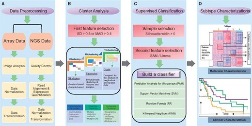
Molecular subtyping of cancer workflow. The workflow consists of four major steps: (A) Data preprocessing. Array data preprocessing include image analysis, data normalization and transformation. Next-generation sequencing data preprocessing contains the following steps: quality control, read alignment, expression quantification, data normalization and transformation. (B) Cluster analysis. A first feature selection is performed with a cutoff on SD (e.g. SD > 0.8) or median absolute deviation (MAD) (e.g. MAD > 0.5). Clustering is usually applied to either feature dimension or sample dimension, biclustering at both dimensions and triclustering at three dimensions (feature, sample and time). After (bi/tri) clustering, the optimal number of (bi/tri) clusters is determined by measurement such as gap statistics, cophenetic coefficients and CDF. Also, ensemble and consensus clustering have been proposed to enhance the robustness of (bi/tri) clustering. (C) Supervised classification. To build the best possible classifier, a sample selection (Silhouette width > 0) and a second feature selection (SAM/Limma) processes are applied. Various algorithms such as PAM, SVM, Random Forests (RF) and K-nearest neighbors can be used to build classifiers. (D) Subtype characterizations. A heatmap is used to represent the molecular characterizations, in which rows are features (genes, miRNAs, pathways, etc.) and columns are samples. Here, features are subtype-specific features; samples are sorted according to their subtype numbers. A Kaplan–Meier survival plot is used to represent the clinical characterizations, in which x-axis is the survival time, and y-axis is the probability of an event (i.e. death).
Subtype identifications
High-throughput molecular data are usually arranged into matrix forms, in which rows are features (genes, miRNAs or DNA methylation markers) and columns are samples. Molecular data matrices have been largely analyzed in two dimensions (2D): the feature dimension and the sample dimension [90]. Clustering is usually applied to either feature dimension or sample dimension. As subsets of features are active or suppressed only under certain experimental conditions, and behave almost independently under other conditions, to identify local patterns in the data matrix, biclustering (or subspace clustering), which allows to discover biclusters, was first proposed by Cheng and Church [91]. Now, various biclustering methods are developed to efficiently identify ‘homogeneous’ submatrices in data, such as singular value decomposition [22], nonnegative matrix factorization (NMF) [23] and geometric-based biclustering [92, 93]. With the fast development of data profiling technologies, it is now possible to have a number of samples for numerous features across multiple time points or experimental conditions. Such data can be arranged into three-dimensional (3D) matrices, with the first two dimensions representing the samples and features, respectively, and the third dimension for time or experimental conditions [94]. To find feature groups along the feature–sample–time (or –condition) dimensions, triclustering is proposed to mine triclusters in the data [95]. As tensor is a concept from mathematics that can be thought of as an organized multidimensional array of numerical values, tensor-based triclustering [96, 97] has become a promising solution for analyzing these longitudinal and spatial data.
The optimal number of clusters is determined by measurements such as gap statistics [98], cophenetic coefficients [99] and cumulative distribution function (CDF). Given that cluster analysis methods are based on different algorithms, they yield different results in terms of cluster numbers and assignments [100]. To enhance the robustness of clustering, a method called cluster ensemble has been proposed, which combines results from different runs of clustering methods into a single consensus result [100]. Another similar methodology is consensus clustering, which in conjunction with resampling techniques provides a method to reach consensus from multiple runs of the same clustering method [101]. The major difference between ensemble and consensus clustering is that ensemble clustering integrates results from multiple clustering methods, while consensus clustering provides resampling and performs a single type of clustering method multiple times. Ensemble and consensus clustering methods are also applicable to biclustering and triclustering, and have been widely used in cancer subtyping studies [19, 20, 46, 102].
Subtype characterizations
Subtype characterizations rely heavily on genomic and clinical data, and one purpose of subtype characterizations is to investigate the associations between the identified subtypes and their molecular/clinical relevance [103]. Subtype characterizations can also help to identify consensus subtypes within and between cancers, which we will cover in detail in ‘Cancer consensus molecular subtypes’ section.
Pathways, mutations, structural variations and methylation patterns can be used as the molecular characteristics. Characterizations of cancer subtypes have implications for patient outcome and targeted therapies. Lex et al. [104] developed an integrative visualization tool called StratomeX, which can help researchers to explore the relationships between subtypes and multiple genomic data types such as gene expression, DNA methylation or copy number data. These genomic data have been discussed in the ‘High-throughput molecular data for cancer subtyping’ section, which can not only be used to identify robust cancer subtypes, but can also help us better understand and interpret the molecular characteristics of the subtypes. In addition, gene set enrichment analysis (GSEA) is usually performed to characterize the biology underlying the identified subtypes. GSEA interprets the expression data at the level of gene sets, groups of genes that share the same biological function, chromosomal location, or regulation [105]. Annotated gene sets with specific biological meanings can be obtained, for example, from Gene Ontology (GO) [106] and KEGG [107] databases.
Clinical data include patient’s information such as age, gender, race, tumor grade, tumor size, time of diagnosis, smoking history, treatment strategies, relapse information, follow-up time and so on, which should be well preserved and managed for clinical characterization of the identified subtypes. Moreover, the survival analysis is a widely used method to compare the survival time differences between subtypes. The Kaplan–Meier estimator [108] can be used to generate the survival curve, and the log rank test provides a statistical comparison of two subtypes [109].
Subtype characterizations are necessary and important. Not only do they help us understand more about the subtype characteristics but also provide a subtype validation process. Ideally, there are distinct molecular and clinical characteristics between identified subtypes. Often, subtypes are only statistically different, but not biologically different. In such cases, reclustering and reclassification should be done until more interpretable results are obtained.
Moving toward clinical applications
From high-throughput molecular data and molecular subtyping of cancer to the development of marker panels using low- and medium-throughput methods, clinicians are beginning to embrace and make treatment decisions for cancer patients based on cancer subtyping studies [110, 111]. In the following, we will provide a few examples of subtyping studies that have been applied to cancer diagnosis, prognosis, response prediction and drug design. Specifically, we will focus on biomarkers for diagnostic and prognostic purposes in ‘Biomarkers identified from subtyping studies for cancer diagnosis and prognosis’ section, and cancer subtypes for therapy response prediction and drug development in ‘Cancer subtypes for predicting therapy response and drug design’ section.
Biomarkers identified from subtyping studies for cancer diagnosis and prognosis
Biomarkers identified from subtyping studies with specific indications for cancer diagnosis and prognosis are now widely applied in clinical research, and increasingly combined with conventional histology to improve diagnostic accuracy [112]. For example, TLE1 as a diagnostic marker for synovial sarcoma [113], and CD10, BCL6 and MUM1 as diagnostic markers for the germinal center B-cell-like (GCB) subtype of lymphoma [114]. Furthermore, biomarkers can be used directly to detect cancer. For instance, Bauer et al. [50] analyzed the complete miRNA repertoire of 136 pancreatic ductal adenocarcinoma (PDAC) samples, 27 pancreatitis samples and 22 normal controls. They used a hierarchical clustering method and an SVM classifier, and found that the analysis of only five miRNAs in blood and tissues can distinguish PDAC from pancreatitis and normal, possibly aiding PDAC diagnosis.
Several multigene predictors have been developed for breast cancer patients [115]. These include MammaPrint, Oncotype DX and simplified MapQuant Dx. These predictors are now widely used in the clinic to classify breast patients and treat them accordingly. MammaPrint was the first successfully applied microarray-based prognostic test for breast cancer. MammaPrint uses a 70-gene signature. To identify these genes, hierarchical clustering was used to classify 98 breast cancer patients into good and poor prognosis groups. This was followed by a three-step supervised classification method to reliably stratify good and poor prognostic categories, and finally found 70 prognostic genes for breast cancer [116]. MammaPrint is a US Food and Drug Administration-approved molecular test to predict the risk of breast cancer metastasis. The result of the test can help physicians to determine the appropriate treatment strategy. Most early-stage breast cancer patients receive adjuvant chemotherapy, but only subset of them benefit from the treatment. Paik et al. [117] thus developed a 21-gene qPCR assay called Oncotype DX. This is a diagnostic test that predicts the likelihood of chemotherapy benefit, and calculates the recurrence scores for early-stage breast cancer. Simplified MapQuant Dx is also a qPCR-based prognostic test for breast cancer. It was developed by Toussaint et al. [118], and is based on the expression patterns of four representative genes from the genomic grade index [119] and four reference genes. The prognostic information provided by the test is only applicable to estrogen receptor-positive breast cancer patients [120].
Cancer subtypes for predicting therapy response and drug design
Subtyping studies are potentially well suited to select a subset of patients that may benefit from certain drugs or therapies. For instance, Rouzier et al. [121] examined if the four subtypes of breast cancer [16] respond differently to chemotherapy. Results showed that the basal-like and ERBB2-overexpressing subtypes are more sensitive to paclitaxel- and doxorubicin-containing preoperative chemotherapy than the luminal and normal-like subtypes.
Tumor specimens for laboratory research are often limited in quantity, infiltrated with nontumor cells and sometimes ethical issues apply. Models for cancer, such as cell lines and patient-derived xenografts (PDXs), have been established as in vitro and in vivo platforms that can overcome these shortcomings of tumor specimens, and are now widely used by researchers. For instance, Ross et al. [122] provided molecular characterization of the NCI (National Cancer Institute)-60 cancer cell line panel, and demonstrated that these cell lines correspond to their tumors of origin. Gao et al. [123] established about 1000 PDXs, which provided excellent in vivo platforms to screen novel therapies for cancer patients. Cancer cell lines and PDXs can also be classified into different subtypes, for example, Kao et al. [124] classified 52 commonly used breast cancer cell lines into five subtypes [42], and defined the cell line subtypes that most faithfully capture the known heterogeneity of breast cancer. Moffitt et al. [51] sequenced 37 PDXs from PDAC and demonstrated that these models can recapitulate tumor-specific subtypes. Therefore, cell line and PDX models can provide a great opportunity to investigate subtype-specific therapies as well.
Recent developments in high-throughput technologies have allowed large-scale screening of chemicals and drugs on cell line panels [125]. For example, the abovementioned NCI-60 cancer cell line panel [126] has been used as a standard platform on which >40 000 chemicals were screened over the past few decades [125]. Besides, Garnett et al. [127] screened a panel of several hundred cancer cell lines with 130 drugs in clinical use and under preclinical investigation, which also provides a powerful strategy to identify subtype-specific cancer therapies and biomarkers to guide such strategies. Drug development is shifting away from cytotoxic agents, to drugs which are designed to target specific molecules that drive the malignant progression [128]. It is still a challenging task, but subtype-specific biomarkers can become potential targets for drug design, and should be investigated and validated further [129, 130].
Challenges
We see four major challenges in cancer subtyping studies that preclude clinical implementation (Figure 2). The first is data acquisition, curation and management. The second challenge is tumor microenvironment (TME) heterogeneity. The remaining two challenges are the lack of consensus molecular subtypes, and problems with single-sample classification, respectively.
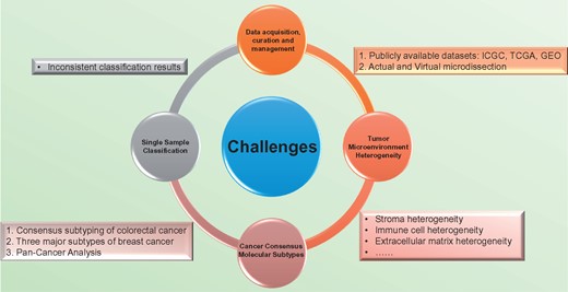
Four major challenges in the molecular subtyping of cancer and associated solutions/problems. The first challenge is data acquisition, curation and management. Data from publicly available data sets, such as ICGC, TCGA and GEO can increase sample size or be used as validation data sets. Low tumor cellularity can be addressed by physical and virtual microdissection. The second challenge is TME heterogeneity. The TME includes immune cells, blood vessels, fibroblasts and ECM, which are all exhibit heterogeneity at some level. The third challenge is the lack of consensus molecular subtypes. Currently, we only have three examples of consensus subtyping studies: colorectal cancer, breast cancer and the TCGA’s pan-cancer study. The last challenge is the problem with single-sample classification. Currently applied SSPs may yield inconsistent classification results.
Data acquisition, curation and management
Many cancer subtyping studies use a strategy called multiple random training-validation strategy [131], in which a training data set is used to identify molecular signatures, and the validation data sets are used to validate the classification performance. Normally, researchers will use their own data set as training data set, and use publicly available data sets as their validation data sets. Publicly available data sets, such as the International Cancer Genome Consortium (ICGC, www.icgc.org) and The Cancer Genome Atlas (TCGA, http://cancergenome.nih.gov/) contain coordinated large-scale cancer genomic data that can be accessed online. ICGC holds genomic, transcriptomic, epigenomic and clinical data from 50 different cancer types and subtypes. Currently, there are >25 000 tumor genome data available on the ICGC website [132]. TCGA also contains a collection of cancer genomic data, and so far, >30 human tumor types have been analyzed through large-scale genome sequencing from 11 000 patient samples [133]. In addition, Gene Expression Omnibus (GEO, http://www.ncbi.nlm.nih.gov/geo/) is a public repository that archives and freely distributes gene expression data from numerous studies [134]. Researchers can upload their own data to the GEO or download data from GEO as validation data sets.
Subtyping studies typically use tumor numbers ranging from dozens to more than few hundreds for their study cohort (Table 2). Identification of cancer subtypes has been frustrated by a lack of tumor samples available for study [19]. For instance, because <20% of PDAC patients have resectable tumors at the time of diagnosis, material for profiling is typically limited [135]. Some studies have overcome this problem by integrating different sources of data into their studies to increase sample size [19, 136]. The introduced batch effects (or nonbiological differences) can be removed by methods like empirical Bayes [137], surrogate variable analysis [138] or Distance Weighted Discrimination [139].
Another common problem is the low tumor cellularity of patient samples, which makes the molecular data noisy. How to capture tumor-specific patterns in such data poses a problem. Because of the tight connection and interaction between cancer cells and surrounding cells, using conventional separation techniques, such as laser capture microdissection [140], cannot perfectly separate tumor cells from nontumor cells. Thus, various statistical enrichment techniques such as virtual microdissection [51], mathematical algorithms like ESTIMATE [141] or qpure [142] can be used to assess tumor cellularity and deconvolve tumor-specific contributions.
In summary, to dissect the genetic heterogeneity of the tumor cell, molecular and clinical data should be well processed and managed. As there are abundant publicly available data sets and various data processing tools that may be useful for answering such questions, researchers should take full advantage of them.
TME heterogeneity
Heterogeneity not only exists in the tumor cell compartment but also in the TME. The TME is the sum of interactions between tumor cells and the surrounding environment, which plays an important role in tumor development, progression and therapy responses. The TME includes immune cells, blood vessels, fibroblasts and extracellular matrix (ECM). Stroma is part of the TME, and is a histological unit consisting of connective tissue, fat tissue, fibroblasts, ECM and immune cells within an extracellular scaffold [143]. Stroma, as a whole, can be classified into different subtypes with clinical implications. For instance, Moffitt et al. [51] used NMF-based consensus clustering of hundreds of PDAC tumors and cell lines, and identified two stroma subtypes named as normal and activated. The activated stroma subtype contributes to poor clinical outcome.
Heterogeneity has also been observed in other components of the TME, such as tumor-infiltrated immune cells, fibroblasts and ECM [144–148]. Solid tumors are infiltrated by various immune cells, for example, T and B lymphocytes, mast cells and so on [149]. These immune cells either play a positive role in inhibition of cancer cell growth or are responsible for the tumor-associated chronic inflammation. The presence of a T-cell-infiltrated TME can serve as a predictive biomarker for response to immunotherapies [144]. However, in many tumor types, only a subset of patients can generate a tumor antigen-specific T-cell response. The remaining patients lack an appropriate T-cell phenotype and resist immunotherapeutic interventions [144]. How to select patients that can potentially benefit from immunotherapies is a challenge. We can address this problem by identifying T-cell response genes and building a binary gene expression classifier, which can distinguish response group from nonresponse group. ECM is a collection of extracellular proteins present in all tissues to provide support to that tissue’s cells [150]. Recent studies have found that considerable heterogeneity exists in the ECM, and clinical outcome is often related with ECM characteristics. For instance, Bergamaschi et al. [147] identified 278 ECM-related genes to classify primary breast tumors into four groups (ECM1–4) with distinct clinical outcomes.
Although tumor and stromal cells have close interactions with each other, stroma cells are different from tumor cells in terms of genetic architecture. Stroma cells are mostly genetically intact [143, 151], which suggests that the stroma could be a target of therapy. Heterogeneity in the characteristic of both tumor cells and TME raise questions regarding future cancer treatment. Which one of them is easier to target? How do we interpret such 2D heterogeneity, and how are they related? Can we incorporate them into a single system? These questions remain to be answered in the future.
Cancer consensus molecular subtypes
Currently, there are six subtyping systems for colorectal cancer (CRC) [20, 46, 45, 47–49], which classify CRC into three to six subtypes (Table 2). To identify robust consensus subtypes of CRCs, a consensus subtyping effort for CRC was initiated. The Colorectal Cancer Subtyping Consortium (CRCSC) developed a network-based approach to investigate the associations between the six independent classification systems. A multi-class classifier was built that could classify CRC into four consensus molecular subtypes (CMS1-4) [152]. CMS1 tumors are highly mutated, microsatellite unstable and show strong immune activation. CMS2 tumors are characterized by marked Wnt and Myc signaling activation. CMS3 cancers are metabolically dysregulated. CMS4 cases feature transforming growth factor-β activation, stromal invasion and angiogenesis signatures. These consensus results will aid future clinical stratification and subtype-based targeted interventions for CRC, and such collaborations should serve as a role model for other cancer subtyping studies to accelerate our understanding of cancer biology [152] and develop more efficient ways to cure cancers.
The use of different patient cohorts, platforms and clustering methods for a specific tumor type, typically yields divergent subtyping results. For breast cancer (Table 2), it was first classified by Perou et al. [16] into four subtypes: luminal, basal-like, normal-like and ERBB2-overexpressing subtypes. Then, Sørlie et al. [42] performed complementary DNA microarrays of 85 breast cancer patients and normal controls, and used hierarchical clustering to classify the patients into one of the five subtypes, i.e. luminal A, luminal B, HER2 over-expression, basal and normal-like. The most recent breast cancer subtyping study by TCGA also suggested four subtypes, which are luminal A, luminal B, HER2-positive and triple-negative subtypes [43]. We can conclude that despite inconsistent naming and number of clusters grouped by different studies [16, 42, 43], breast tumors fall primarily into three major subtypes: luminal, HER2 overexpression and triple-negative breast cancer (TNBC) [89]. The luminal subtype cancer is the most common one and carries a good prognosis. This subset of patients expresses hormone receptors, and this makes them responsive to hormone therapies. The HER2-overexpressing breast cancer subtype is more sensitive to herceptin (trastuzumab) and chemotherapy than the luminal subtype. The TNBC subtype is resistant to standard targeted therapies, and carries the worst prognosis.
The next important consideration is the consensus subtyping between cancers. Although there are many cancer types based on their tissue of origin, we can observe similarities between them. The TCGA’s pan-cancer classification study [32] is a good example of this. Six different ‘omic’ platforms were integratively analyzed, consisting of 3527 tumor specimens across 12 cancer types. A unified cancer classification system was constructed, and it identified 11 major subtypes. Among them, five subtypes were strongly associated with their tissue of origin, but the remaining subtypes were not strictly associated with their tissue of origin. For instance, bladder cancers split into three pan-cancer subtypes. Lung squamous, head and neck and a subset of bladder cancers coalesced into a single subtype. This study not only provided a new classification system for multiple cancers but also demonstrated that general characteristics exist between cancers that were traditionally considered to be different entities.
Cancer is a complex disease. Without a systematic understanding of the characteristics of the disease, we cannot develop effective therapies against it. The general characteristics within and between cancers provide great opportunities to identify consensus molecular subtypes. For example, basal subtypes are defined in breast cancer [42], bladder cancer [88] and pancreatic cancer [51]. Mesenchymal subtypes are defined in glioblastoma (GBM) [41], NPC [15], breast [153], pancreatic [19] and colon cancers [20]. Basal subtypes usually express genes like laminins and keratins, and have the worst prognosis compared with other subtypes. The characteristics of mesenchymal subtypes include a mesenchymal phenotype, high expression of proliferation genes, poor prognosis, high malignant potential and resistance to current therapies. Thus, devise treatments that are effective against multiple cancer types with shared characteristics may become a promising solution for future cancer treatment.
Single-sample classification
The abovementioned classifiers (or predictor) are mainly built based on a large number of training samples, and for this reason, we call them population-based predictors. In contrast, single-sample predictors (SSPs) are classification models that can classify a single sample into one of the molecular subtypes of a specific type of cancer [154, 155]. Traditionally, to classify a new sample into a specific subtype based on population-based predictor, reanalysis of a large data set is needed. Contrary to the population-based predictor, SSPs can assign a single sample to a specific subtype regardless of other samples, and is therefore more useful and practical for individual patients than population-based predictors. SSPs have been built for several types of cancer. For instances, Sørlie et al. [154] constructed the first SSP for breast cancer, Stratford et al. [136] developed an SSP for PDAC and Ringnér et al. [156] derived an SSP for lung adenocarcinoma.
SSPs are constructed based on tumor-intrinsic signatures and similarities between a given sample and molecular subtype centroids [154, 155]. Methods applied in the population-based predictor, such as hierarchical clustering and nearest centroid classification method [157], can be used in the SSP. One of the most important requirements for an SSP is that it cannot be built based on row-centered (mean centering or median centering) data [158]. Normally, molecular data matrices contain features in rows and samples in columns. Row-centering is a feature centering process that can help to remove side effects caused by outlier features. The construction of SSPs features no row-centering step, and studies have found inconsistent classification results caused by SSPs [158–160]. Sørlie et al. [161] accepted Weigelt et al.’s [158] conclusions and comments, and explained why there were inconsistent classification results. The reasons are listed below: for the three one-channel-based data sets, most of the variations were caused by differences between genes, and not so much by differences between samples. So, the correlation values vary greatly over a smaller range in the uncentered data. Therefore, for a sample to be correctly assigned to a subtype, it must be centered against an appropriately large and heterogeneous sample set. Sørlie et al. [161] highlighted the importance of performing row-centering in molecular data-processing steps.
In summary, building SSPs is a challenging but important task, and up to now, there are no effective ways to deal with the centering problem. Although current results are not encouraging, we hope that in the near future, applicable SSPs can be developed and applied in the clinic.
Conclusions and outlook
Heterogeneity renders cancer more than a single disease. This poses a significant challenge to the traditional management of cancer. With the advent of genome-wide molecular profiling of cancer, especially the advancements in high-throughput profiling technologies, researchers can now investigate the collective of genomic and epigenomic changes that exist in cancer. In contrast with traditional classification methods, molecular classification can be used to assign cancers to subgroups with distinct molecular characteristics, tumor biology and clinical presentation.
The most important step in molecular subtyping of cancer is cluster analysis. Different clustering methods can produce different results, many cluster analyses are unstable and cluster analyses are a purely exploratory method [162]. It is hard to tell which algorithm is better, as this largely depends on the question asked. Thus, it is important to ascertain proper preprocessing and normalization of the data; also, ensemble and consensus clustering methods should be considered when doing the cluster analysis. Another important step is subtype characterizations. The identified subtypes should be both statistically significant and biologically relevant. This means that molecular as well as clinical data collection is mandatory to truly characterize the identified subtypes. Also, publicly available data sets can be used to evaluate the classification performance of the classifiers.
Although numerous molecular subtyping studies have been conducted, which have identified subtypes for various cancer types, current cancer patient stratification still largely relies on traditional histopathological observation and assessment. We are facing several challenges (Figure 2). The gap between research findings (identified subtypes) and clinical applications can be bridged by the improvement of statistical methods and better interpretation of the results. When cancers are correctly separated into different subtypes, the next important step is to properly interpret these identified subtypes from a biological point of view followed by a move toward clinical applications. With the successfully applied clinical tests in breast cancer, we hope that this will be followed in other cancer types.
In summary, cancer should not be treated as single disease. Molecular subtyping can identify distinct cancer subtypes, which may shed new lights on the treatment strategies for cancer patients. Several challenges should be addressed before clinical applications can be successfully applied.
Heterogeneity renders cancer more than a single disease. Molecular subtyping can be used to assign cancers to subgroups with distinct molecular characteristics, tumor biology and clinical presentation.
Unsupervised classification schemes have been successfully applied to identify subtypes in a large number of malignancies. From these studies, we summarize a workflow for molecular subtyping of cancer. These include data preprocessing, cluster analysis, supervised classification and subtype characterizations.
We identified and described four major challenges in cancer subtyping studies that preclude clinical implementation. The first is data acquisition, curation and management. The second challenge is TME heterogeneity. The remaining two challenges are the lack of consensus molecular subtypes, and problems with single-sample classification, respectively.
We suggest that standardized methods should be established to help identify intrinsic subgroup signatures and to build robust classifiers that pave the way toward stratified treatment of cancer patients.
Lan Zhao is a PhD candidate at the Department of Electronic Engineering, City University of Hong Kong. Her research interests are in the areas of machine learning, cancer genomics and computational biology.
Victor H. F. Lee is currently a Clinical Associate Professor of the Department of Clinical Oncology, the University of Hong Kong. His current interests include clinical and genetic studies on nasopharyngeal cancer, head and neck cancers, lung cancers, liver cancers and gastrointestinal cancers.
Michael K. Ng is the Head and Chair Professor of the Department of Mathematics, and Chair Professor (Affiliate) of Department of Computer Science at the Hong Kong Baptist University. As an applied mathematician, his main research areas include bioinformatics, data mining, operations research and scientific computing.
Hong Yan received his PhD degree from Yale University. He was a Professor of imaging science at the University of Sydney and currently is the chair professor of computer engineering at City University of Hong Kong. His research interests include bioinformatics, image processing and pattern recognition.
Maarten F. Bijlsma is an Associate Professor at the Academic Medical Center with the University of Amsterdam. His research focuses on pancreatic and esophageal cancer, from the most fundamental mechanisms that underlie aberrant signaling in these diseases, to the development of serum-borne markers in patient cohorts to predict treatment response and disease outcome. Furthermore, he is a Biomarker/Imaging Program leader for the AMC/VUmc Cancer Center Amsterdam.
Acknowledgement
The authors thank Xin Wang from Department of Biomedical Sciences of the City University of Hong Kong for comments on an earlier version of the manuscript.
Funding
This work was supported by Hong Kong Research Grants Council (RGC) (Project C1007-15G) and City University of Hong Kong (Project 7004862).
