


Abstract
The genomes of mammalian species are pervasively transcribed producing as many noncoding as protein-coding RNAs. There is a growing body of evidence supporting their functional role. Long noncoding RNA (lncRNA) can bind both nucleic acids and proteins through several mechanisms. A reliable computational prediction of the most probable mechanism of lncRNA interaction can facilitate experimental validation of its function. In this study, we benchmarked computational tools capable to discriminate lncRNA from mRNA and predict lncRNA interactions with other nucleic acids. We assessed the performance of 9 tools for distinguishing protein-coding from noncoding RNAs, as well as 19 tools for prediction of RNA-RNA and RNA-DNA interactions. Our conclusions about the considered tools were based on their performances on the entire genome/transcriptome level, as it is the most common task nowadays. We found that FEELnc and CPAT distinguish between coding and noncoding mammalian transcripts in the most accurate manner. ASSA, RIBlast and LASTAL, as well as Triplexator, turned out to be the best predictors of RNA-RNA and RNA-DNA interactions, respectively. We showed that the normalization of the predicted interaction strength to the transcript length and GC content may improve the accuracy of inferring RNA interactions. Yet, all the current tools have difficulties to make accurate predictions of short-trans RNA-RNA interactions—stretches of sparse contacts. All over, there is still room for improvement in each category, especially for predictions of RNA interactions.
Introduction
Studies of transcriptomes have demonstrated that transcription is pervasive in higher organisms and produces a wide variety of noncoding RNAs [1, 2] including relatively well-studied small RNAs, such as microRNAs or piRNAs (reviewed in [3]), and a much less studied long noncoding RNA (lncRNA). Classically, lncRNAs are defined as transcripts longer than 200 nt without any protein-coding capacity. LncRNAs are usually low expressed and highly tissue-specific in comparison with protein-coding genes, which leads to difficulties in robust detection of their transcription as well as detailed reconstruction of the transcript structure [4, 5]. Combination of several RNA-sequencing techniques has helped to solve this problem [6, 7]. Currently, the total number of lncRNAs annotated in the human and mouse genomes is close to the number of protein-coding genes [8, 9].
Despite the progress in the identification of the transcribed regions of mammalian genomes, not all newly found genes are reliably annotated. In particular, regions initially considered as noncoding appeared to be protein-coding after proteomics studies have identified short peptides produced from these transcripts [10, 11]. On the other hand, it has been suggested to revise the current human protein-coding gene catalog and classify some of the genes as noncoding [12]. Therefore, wet-lab researchers studying the function of a particular lncRNA face a challenging problem to ensure that the transcript in question is indeed non-coding. This is especially relevant to the non-model organisms with poorly annotated transcriptomes.
LncRNAs are among the fastest evolving functional units of the genome [13] (reviewed in [14]); for instance, one-third of the human lncRNAs are thought to have arisen solely in the primate lineage [15]. Consequently, the evolutionary conservation of lncRNA sequences is generally fairly low [15]. Single-stranded ribonucleotide chains (including lncRNAs) tend to fold into thermodynamically stable structures [16]. In many cases, the secondary structure of lncRNAs dictates their function (reviewed in details in [17]). Yet, at least some of the functional lncRNAs lack structural conservation [18], which reduced the role of conservation in lncRNA detection. Interestingly, many of them (e.g. promoter upstream transcripts, PROMPTs [19] and enhancer RNAs [6, 20]) originate from regulatory regions of other genes making the act of transcription more functionally relevant than the transcript produced.
The current lncRNA classifications are usually based not on their intrinsic features but rather on their relationship to the protein-coding genes. One of the most frequently used classifications was proposed by GENCODE [15] and included the following categories: (i) antisense RNAs, (ii) long intergenic noncoding RNAs (lincRNAs), (iii) sense overlapping transcripts, (iv) sense intronic transcripts and (v) processed transcripts. Among >15 000 human lncRNA genes annotated in the GENCODE version 27, 48 and 35% belong to the intergenic and antisense types, respectively. For the purpose of this benchmarking study, we will focus on these two categories, as they correspond to the majority (83%) of known lncRNAs. Summing up, computational annotation of lncRNA is a challenging task because of lack of known intrinsic properties typical for all lncRNAs, complex structures and poor evolutionary conservation.
The fact that transcription of lncRNAs is regulated suggests their functionality [6, 21]. Indeed, it has been shown that they function via surprisingly diverse molecular mechanisms on the transcriptional and posttranscriptional levels (reviewed in [22, 23]). LncRNAs are often located in the nucleus of the mammalian cells [24] and mediate transcription by directing chromatin modifying complexes [25, 26] or transcription factors (TFs) [27] to specific genomic loci. They use different molecular mechanisms to bind to the chromatin, including direct RNA-DNA hybridization via triplexes [28, 29], RNA binding to unpaired (single-stranded) DNA regions (known as R-loops) [30], co-transcriptional RNA-RNA interactions [31] and RNA-DNA binding mediated by protein complexes.
RNA has the capacity to form hydrogen bonds on the Watson–Crick face—forming both Watson–Crick and non-Watson–Crick pairs [32]—but also the Hoogsteen bonds. LncRNAs can bind promoter regions and participate in transcription regulation [33]. Several studies have reported triplex formation by lncRNA HOTAIR [34, 35], Fendrr [25], MEG3 [26], PARTICL [36].
On the other hand, there are multiple known cases of regulatory intermolecular RNA-RNA binding within nucleus and cytoplasm, which are usually classified into two groups—cis and trans. The interactions of the first type occur between the products of the overlapping genes transcribed in opposite directions. The resulting RNAs have one or several sites perfectly complementary to each other [37]. All other interactions are classified as trans (‘not-cis’), as they are formed between the transcripts originated from different genomic loci. Even trans-interactions can be based on long, highly complementary RNA duplexes because of the expressed paralogous genes (we refer to such interactions as ‘pseudo-cis’ [38]) or widespread genomic repeats (e.g. Alu-based binding [39]). Finally, intermolecular hybridization between long RNAs can be based on relatively short regions of complementarity (‘short-trans interactions’). Examples of cytoplasmic lncRNAs that form interactions of this type include TINCR [40] and lincRNA-p21 [41]. In the nucleus, in addition to forming a triplex with DNA, lncRNA HOTAIR can also bind to specific genomic loci by hybridization with the nascent transcripts presumably via short-trans base pairing [31].
Accurate detection of the targets bound by a particular lncRNA may facilitate its functional annotation. Given a wide range of possible binding mechanisms [42], a working hypothesis is needed to efficiently choose the direction for the future experiments. This is where computational predictions may help.
In the current study, we compared tools capable of answering two important questions of lncRNA biology. First, whether a long transcript of interest is indeed a noncoding. Second, how does it interact with its nucleic acids targets? Here, we consider available bioinformatics tools developed to predict two possible RNA interaction mechanisms: intermolecular RNA-RNA hybridization and formation of RNA-DNA triplexes. Computational prediction of RNA–protein interactions have recently and thoroughly been reviewed elsewhere [43, 44]. In the case of RNA:DNA hybrid in the R-loops, the interaction occurs via Watson–Crick base-pairing rules [30, 45]. So the main challenge of the genome-wide RNA:DNA duplex prediction is to determine loci where DNA helix is open and single-stranded DNA is accessible, which falls beyond the scope of the present study. For our benchmark, we collected several lncRNA sets with experimentally verified properties (functions and interactions). Making our conclusions, we gave priority to the tests that showed tool performances on the entire genome/transcriptome level—the task of the highest interest in the current era of high-throughput sequencing.
Tools
RNA classification
The majority of known lncRNAs are generated by the same transcriptional machinery as mRNAs, as it follows from RNA PolII and TF occupancy [21], typical promoter histone modification profile [46] and presence of a 5′ terminal cap [6]. In this regard, the first question is how to reliably distinguish protein-coding and noncoding RNAs at the level of the whole transcriptome. In this study, we refer to this task as ‘RNA classification’. It should be noted that an RNA may encode a protein and at the same time have an additional nonprotein-coding function [47, 48]. Such ‘dual-function’ RNAs are the most difficult to determine. There are only few known cases of such RNAs, and computational tools to identify them have not been yet developed.
One of the ways to solve the RNA classification problem is to computationally identify all protein-coding RNAs and assume that all the remaining long transcripts are lncRNAs. A number of algorithms can be used for this task. Roughly, all of them can be classified into two major groups—the ones that take advantage of the database search (the ‘homology-‘ or ‘alignment-based’ methods) and the ones that only rely on the intrinsic properties of the given nucleotide sequences (the ‘ab initio’ or ‘alignment-free’ methods). We did not include the alignment-based tools (such as CPC [49] and PhyloCSF [50]) in our benchmark because the quality of their predictions depends heavily on the presence of homologs in protein databases. It should be noted that plant-specific ab initio approaches (such as PlncPRO [51]) were not included as well. Therefore, in this work, we considered general alignment-free tools only (Table 1).
Some of the features of the evaluated RNA classification tools.
| Software name | Software version | Prediction measure | Strategy | Model parameters | Explicit class label | Parallel computing | Web server | Reference |
|---|---|---|---|---|---|---|---|---|
| CNCI | 2 | S-score | Support Vector Machine (SVM) | Pre-built models (vertebrates, plants) | ✓ | ✓ | ✗ | [52] |
| CPAT | 1.2.2 | Coding probability | Logistic Regression | Pre-built models (human, mouse, drosophila, zebrafish) | ✓a | ✗ | ✓ | [53] |
| ESTScan | 3.0.3 | Score | Hidden Markov Model (HMM) | Pre-built models (human, mouse, rat, zebrafish, drosophila, rice, maize, arabidopsis) | ✓b | ✗ | ✓ | [54] |
| FEELnc | 0.01 | Coding potential score | Random forest | Supervised training | ✓ | ✗ | ✗ | [55] |
| GeneMarkS-T | 5.1 | Gene score | HMM | Unsupervised self-training | ✓b | ✗ | ✗ | [56] |
| PLEK | 1.2 | Score | SVM | Pre-built models (vertebrates, plants) | ✓ | ✓ | ✗ | [57] |
| PORTRAIT | 1.1 | Coding probability | SVM | Pre-built model (universalc) | ✓ | ✗ | ✗ | [58] |
| Prodigal | 2.6.3 | Score | Dynamic programming | Unsupervised self-training | ✓b | ✗ | ✗ | [59] |
| TransDecoder | 3.0.1 | – | HMM | Supervised training | ✓b | ✗ | ✗ | [60] |
Note: Column notation: Prediction measure—the values used in our study to rank the tool predictions, strategy—the classification/prediction algorithm used by the tool, model parameters—how the parameters of the prediction model are estimated (the tool may include taxa-specific pre-built models, it may require a set of sequences for supervised training or it may perform unsupervised self-training on the input data), parallel computing—whether the tool is able to use multiple threads, Web server—whether a functional Web server is available for the tool.
aCPAT produces predictions for all the input sequences without explicit class labels, but the authors provide a set of recommended species-specific thresholds, which were used in our study.
bA transcript is considered to be protein-coding if at least one CDS is predicted by the tool, and noncoding—otherwise.
cPORTRAIT ‘universal’ model has been trained on a large set of sequences from the SwissProt, RNAdb, NONCODE and rfam databases.
All the considered tools take advantage of the fact that lncRNAs lack features associated with the ability to encode proteins, such as presence of relatively long open reading frames with the typical species-specific codon usage. The codon usage is usually taken into account by computing frequences of various k-mers and incorporating this information (along with some other features) into a prediction algorithm. The algorithmic differences between the approaches can be found in Table 1 (see the ‘Strategy’ column). Three tools (ESTscan, GeneMarkS-T and TransDecoder) incorporate the k-mer frequencies into a hidden Markov model (HMM)—the approach proved to be successful for gene finding in prokaryotic genomes—and use it to find the coding regions. Prodigal uses a custom formula to compute a coding score from the k-mer frequencies. This tool has been developed for prokaryotic genomes; however, we use its ‘switched-off RBS model’ option (see Supplementary Materials), which allows to get the predictions for eukaryotic transcripts. More recently developed approaches compute a number of features from each input sequence. The transcripts are then considered as points in a multidimensional space and one of the classical machine learning algorithms—support vector machine (CNCI, PLEK, PORTRAIT), logistic regression (CPAT), random forest (FEELnc)—is used for classification. It should be noted that these tools either directly use the k-mer frequencies as transcript features or first combine them to compute a coding score that is used as one of the features on the classification step.
The tools also differ in the way the model parameters are estimated (i.e. supervised versus unsupervised training). Several tools included in our analysis (CNCI, CPAT, ESTScan, PLEK, PORTRAIT) have species- or taxa-specific pre-built models and do not require a training set for parameter optimization. These models have been obtained via supervised training on large sets of transcripts with known type. Other tools (FEELnc, TransDecoder) require a separate set of annotated RNAs for supervised training. Finally, GeneMarkS-T and Prodigal implement unsupervised self-training that optimizes the model parameters via iterative learning on the input data.
It should also be noted that some tools (e.g. GeneMarkS-T) aim to predict the borders of the coding region (CDS) within each mRNA, while other tools simply classify a transcript into a protein-coding and noncoding category. In this benchmark, we do not evaluate the accuracy of the CDS coordinates and only consider the predicted transcript labels.
RNA-RNA interaction prediction
The problem of intermolecular RNA-RNA interaction prediction has been studied extensively producing multiple computational tools. Yet, to the best of our knowledge, the benchmark of the tools has been performed with the focus on the microbial RNA interactions [61, 62]. Here, we performed a comparison with the focus on the mammalian RNAs. To this end, we evaluated all general purpose RNA-RNA interaction prediction tools, which use the information about RNA sequence only. Note, we did not consider miRNA target prediction programs, as the features implemented to account for mechanistic details of miRNA biogenesis and functioning (such as requirement for the miRNA seed match) may not be relevant for lncRNAs and mRNAs.
There is a group of RNA-RNA interaction prediction tools (RNAaliduplex [63], PETcofold [64]) that take multiple sequence alignments as input. Such tools search for conserved intermolecular duplexes supported by coordinated nucleotide substitutions (covariations). We did not include such tools in our study, as the reliable information about lncRNA homologs is currently limited. Also, we did not consider tools that only output free energy for the whole RNA-RNA complex, rather than for the intermolecular duplexes only (such as PairFold [65] and RNAcofold [66]).
Some important features of the tools included in our benchmark are summarized in Table 2. Following the excellent review by Lai and Meyer [62], we classified all the algorithms into five types. Briefly, the ‘Interaction only’ category includes tools that predict intermolecular hybridization (i.e. sense-antisense interaction) without considering intramolecular base pairing (i.e. RNA secondary structures are ignored). Local sequence alignment tools do not take secondary structure into account as well. However, we use a separate ‘Alignment’ category for them to emphasize that originally they have been developed for that purpose. The tools in the ‘Accessibility’ category account for the RNA secondary structures by using a partition function to estimate the probability of each nucleotide to be unpaired. The ‘Complex joint’ category includes the tools aiming to comprehensively predict the joint secondary structure of two RNA molecules allowing both intramolecular and intermolecular interactions. This type of tools are able to predict complex RNA-RNA binding (such as the ‘kissing hairpins’) at the cost of larger execution time. More recently, several tools have been developed for predicting RNA-RNA interactions on a large scale (e.g. transcriptome-wide) by combining the local alignment and the secondary structure aware algorithms (the ‘Alignment + Accessibility’ category). The sequence alignment step allows these approaches to restrict the prediction or intramolecular and intermolecular interactions to a smaller set of local regions of the long transcripts.
Some of the features of the evaluated RNA-RNA interaction prediction tools.
| Software name | Software version | Prediction measure | Strategy | G-U base pairing | Secondary structure | Stat. significance | Parallel computing | Web server | Reference |
|---|---|---|---|---|---|---|---|---|---|
| AccessFold | 5.8.1a | Δ G | Accessibility | ✓ | ✓ | ✗ | ✗ | ✗ | [67] |
| ASSA | 1.00 | log(P-value) | Alignment + Accessibility | ✓ | ✓ | ✓ | ✓ | ✗ | [68] |
| Bifold | 5.8.1a | Δ G | Complex joint | ✓ | ✓ | ✗ | ✗ | ✓ | [69] |
| BLASTn | 2.3.0+ | log(min(E-value)) | Alignment | ✗ | ✗ | ✓ | ✓ | ✓ | [70] |
| DuplexFold | 5.8.1a | Δ G | Interaction only | ✓ | ✗ | ✗ | ✗ | ✓ | [71] |
| GUUGle | 1.2 | Longest duplex length | Interaction only | ✓ | ✗ | ✗ | ✗ | ✓ | [72] |
| IntaRNA2 | 2.0.4 | Δ G | Accessibility | ✓ | ✓ | ✗ | ✗ | ✓ | [73] |
| IRIS | 4.1 | Δ G | Complex joint | ✓ | ✓ | ✗ | ✗ | ✗ | [74] |
| LASTAL | 864 | log(min(E-value)) | Alignment | ✓ | ✗ | ✓ | ✓ | ✓ | [75] |
| LncTar | April-2015 | ndG (normalized Δ G) | Complex joint | ✓ | ✓ | ✗ | ✗ | ✓ | [76] |
| RactIP | 1.0.1 | Δ G | Complex joint | ✓ | ✓ | ✗ | ✗ | ✓ | [77] |
| RIblast | 1.1.2 | SumEnergy | Alignment + Accessibility | ✓ | ✓ | ✗ | ✗ | ✗ | [78] |
| RIsearch2 | 2.0 | Δ G | Interaction only | ✓ | ✗ | ✗ | ✓ | ✗ | [79] |
| RNAduplex | 2.2.10b | Δ G | Interaction only | ✓ | ✗ | ✗ | ✗ | ✗ | [63] |
| RNAplex-a | 2.2.10b | Δ G | Accessibility | ✓ | ✓ | ✗ | ✗ | ✗ | [80] |
| RNAplex-c | 2.2.10b | Δ G | Interaction only | ✓ | ✗ | ✗ | ✗ | ✗ | [81] |
| RNAup | 2.2.10b | Δ G | Accessibility | ✓ | ✓ | ✗ | ✗ | ✓ | [82] |
| RRP | 0.1 | SumEnergy | Alignment + Accessibility | ✓ | ✓ | ✗ | ✗ | ✗ | [83] |
Note: Column notation: Prediction measure—the values used in our study to rank the tool predictions, strategy—the broad strategy of the algorithm (see text for more details), G-U base pairing—whether the wobble base pair is included in the hybridization rules, secondary structure—whether the RNA secondary structures (i.e. intramolecular interactions) of the input RNAs are taken into account, stat. significance—whether the tool provides a statistical significance estimate for each prediction, parallel computing—whether the tool is able to use multiple threads, Web server—whether a functional Web server is available for the tool.
aRNAstructure package.
bViennaRNA package.
We included two sequence alignment tools (LASTAL and BLASTn) in our benchmark, as they have previously been used in transcriptome-wide searches for the natural antisense transcripts [84, 85]. They estimate the strength of their hits by a statistics-based measure (E-value). All other tools in our benchmark output free energy (ΔG) as a thermodynamics-based measure of the RNA-RNA interaction strength. Some of the tools (RIblast, RRP) predict several intermolecular duplexes for a transcript pair. In such cases, we sum all the ΔG values to obtain the SumEnergy, as it has been shown to produce more accurate predictions [83]. On the other hand, it has been shown that interaction energy depends on the features (length and GC content) of the input sequences [68]. LncTar and ASSA take this into account by computing ‘normalized Δ G’ and ‘theoretical p-value’, respectively. It should be noted that ASSA is the only tool that outputs interaction free energy together with an estimate of its statistical significance. We used the log(P-value) to rank its predictions.
For many prokaryotic small RNA-mRNA interactions the hybridization regions have been determined experimentally. Lai and Meyer [62] have used this information to compare different computational tools based on the overlap between the predicted and the known locations of intermolecular duplexes. However, such information is not usually available for the interactions between mammalian long RNAs. Therefore, in this study, we were focused on another important task—identification of the potential targets without considering the predicted regions of intermolecular complementarity. Our goal here was to compare the existing computational tools by their ability to reconstruct the experimentally established RNA interactomes (see below).
RNA-DNA triplex prediction
Up until now, computational prediction of RNA-DNA interactions attracted relatively little attention. We found only a few tools developed to assess RNA-DNA triple helix formation: Triplexator [86], LongTarget [87], Triplex Domain Finder (TDF) [88], Triplex [89] and Triplex-Inspector [90]). Triplexator considers Hoogsteen and reverse-Hoogsteen base-pairing, while LongTarget in addition to the Hoogsteen-based hybridization includes a number of non-canonical base-pairing rules (detailed comparison of the tools is available in Table 3). TDF is based on the triplexes, predicted by Triplexator. It evaluates statistically the triplex forming potential of a particular RNA in multiple DNA regions and ranks the DNA regions by its RNA binding affinity. As TDF does not improve triplex prediction per se, we excluded TDF from the comparison. Triplex-Inspector is also based on Triplexator predictions and addresses a specific question of generation an lncRNA sequence capable of forming a triplex with a DNA region of interest. Therefore, Triplex-Inspector was not included in the comparison. Several other tools, such as TTSmapping [91] or a method developed by Hoyne et al. [92], focus on finding DNA regions capable of triplex formation (triplex target sites, TTS) without considering the sequence of potentially interacting RNA, so we did not include such methods into the benchmark.
Some of the features of the RNA-DNA triplex prediction tools.
| Software name | Software version | Prediction measure | Number of base-paring rules | Number of TFO per RNA | Triplex stability estimate | Length normalization | Search optimization | Parallel computing | Reference |
|---|---|---|---|---|---|---|---|---|---|
| LongTarget | 4.0.1 | SumScore | 16 | Single best hit | ✓ | ✗ | ✗ | ✗ | [87] |
| Triplexator | 1.3.2 | SumScore | 6 | Multiple independent hits | ✗ | ✓ | ✓ | ✓ | [86] |
Note: Column notation: Prediction measure—the values used in our study to rank the tool predictions. Triplex stability estimate is performed by LongTarget by summing up the experimental estimated stabilities of the RNA triplets. Length normalization in Triplexator is performed by introducing triplex potential. For the search optimization, Triplexator can use q-gram to quickly filter out non-hits at expense of the increased RAM use. Triplexator can take an advantage of using OpenMP and running in parallel mode.
Summing up, we assessed the performance of LongTarget and Triplexator, the only developed tools to predict intermolecular RNA-DNA triplexes. As Triplexator can use only a subset of base-pairing rules, we used it in six different modes: the default with all rules enabled and with the ‘-m’ option assigned to one of the five allowed values R, Y, M, P or A (see the ‘Tool settings’ section in the Supplementary Materials).
Methods
Training and test sets for RNA classification
In this work, we evaluated the ability of the tools to classify transcripts as protein-coding or noncoding on several test sets. To evaluate how well the tools generalize to different mammalian genomes, we prepared test sets from two different species—human and mouse. The human GENCODE annotation version 25 (for hg38 genome) includes 19 729 protein-coding and 13 058 long noncoding (the ‘lincRNA’ or ‘antisense’ biotypes) genes. The mouse GENCODE annotation version M12 (for mm10 genome) includes 21 909 protein-coding and 6674 long noncoding (the ‘lincRNA’ or ‘antisense’ biotypes) genes. After the additional validation of the lncRNAs with BLASTx (see Supplementary text), we randomly selected 1000 human and 1000 mouse lncRNA genes (only the longest isoform of each lncRNA gene was used, Figure 1B).
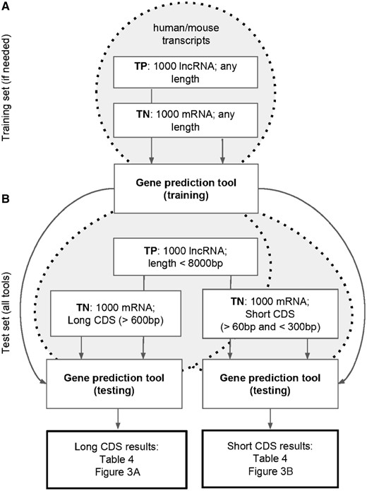
Training and test sets for RNA classification tools. (Top) The training set was used to generate species-specific models for the tools that require a supervised training (FEELnc and TransDecoder). (Bottom) Each RNA classification tool was applied to the sequences from two types of test sets (i.e. containing long- and short-CDS mRNAs), and the performance statistics were calculated. Note that for a given species, both test sets included the same 1000 lncRNAs sequences. TP: true positive; TN: true negative.
Owing to the algorithmic details of the alignment-free tools, better performance can be expected on the mRNAs with relatively long CDSs. To study the ability of the algorithms to work with transcripts containing CDSs of any length, we generated two types of test sets by combining the 1000 selected lncRNA sequences with either the ‘long-CDS’ or the ‘short-CDS’ mRNAs (see Supplementary text). In total, the four test sets (Human Long-CDS, Human Short-CDS, Mouse Long-CDS and Mouse Short-CDS) were generated with each test set consisting of 2000 transcripts (1000 mRNAs + 1000 lncRNAs, Supplementary Figure S1). Additionally, two training sets (for human and mouse) were prepared by randomly selecting the longest isoforms of 1000 protein-coding and 1000 noncoding human and mouse genes that were not present in the prepared test sets (Figure 1A). See the Supplementary text for the details on how the evaluation metrics [Matthews correlation coefficient (MCC) and area under the receiver operating characteristic (ROC) curve (AUC)] are computed based on the predictions of each tool.
Test sets for RNA-RNA interaction prediction
We envisioned three scenarios of the RNA-RNA interaction prediction tool usage (Figure 2A). In the ‘one-vs-one’ mode, we investigated the ability of different tools to distinguish the experimentally validated interactions between real transcripts from the interactions that may happen by chance between random sequences with similar properties. Specifically, from the literature survey, we manually collected experimentally validated cases of intermolecular hybridizations between long transcripts (lncRNA or mRNA). As some of the tools require significant amount of RAM to process long RNAs, we limited our analysis to the 17 interactions between transcripts shorter than 5000 nt (Supplementary Table S1). First, every tool was used to compute the interaction strength for each transcript pair. Next, the statistical significance was assigned to each obtained value by computing empirical P-value (see Supplementary text).
![Test sets for (top) RNA-RNA and (bottom) RNA-DNA interaction prediction tools. (Left) The ‘one-vs-one’ category included a number of specific RNA-RNA (top left) or RNA-DNA (bottom left) pairs collected from various publications. Importantly, both the query and target sequences were different between the pairs. The false interactions were simulated by dinucleotide shuffling the RNA sequences. (Middle) The ‘one-vs-many’ test sets included only one query lncRNA [TINCR (top middle) and MEG3 (bottom middle) in case of RNA-RNA and RNA-DNA interactions, respectively] and many different target sequences. Randomly selected transcripts/genomic regions were used as false targets. Additional RNA-RNA interaction prediction testing was done by using di-nucleotide shuffled sequences as false targets. Note that the same true RNA targets were used in both the TINCR ‘one-vs-many’ test sets. (Top right) Finally, the ‘many-vs-many’ test set was prepared to evaluate the ability to reconstruct global RNA-RNA interaction network. This test set type is similar to the ‘one-vs-one’ in that both the query and target were different between the true transcript pairs. However, all these bindings were identified within a single high-throughput experiment (SPLASH). Moreover, in the ‘many-vs-many’ test set, any transcript pair not identified by the SPASH method was considered as a false interaction. (A) Human long-CDS test set and (B) human short-CDS test set. TP: true positive; TN: true negative.](https://oup.silverchair-cdn.com/oup/backfile/Content_public/Journal/bib/20/2/10.1093_bib_bby032/8/m_bby032f2.jpeg?Expires=1750246050&Signature=J8JJv3~PboJ88Vxx14lSyHzHVXaDoHwD80mNjpbXWt0iOsSzfbSuwiX-Alvr~hq1g7Su~QQMsFaCYmjwFUXLAT-FdxPVpuDRa9nB21p~dFu5e9wiUdRXPvRTIZKdv3CAzxtAxaYsPav63cKmmL2i0VDlwcQyy97QKGdaq5ZKhkhdT7TsqXDuVPVh2viwCDI46q5ldAApTTALflM~GiqmFu38Ocwl-oaMnf81NClGGpfqx3iLkfssVC235L7vt4cGq9qEvCMHU31Jn9KaJZ8N3XmA41oBQDlvLSWAaoYn556OZHKsT~U5NkQxA3qr0oA-t860GR2903OPDTc-l~i9mQ__&Key-Pair-Id=APKAIE5G5CRDK6RD3PGA)
Test sets for (top) RNA-RNA and (bottom) RNA-DNA interaction prediction tools. (Left) The ‘one-vs-one’ category included a number of specific RNA-RNA (top left) or RNA-DNA (bottom left) pairs collected from various publications. Importantly, both the query and target sequences were different between the pairs. The false interactions were simulated by dinucleotide shuffling the RNA sequences. (Middle) The ‘one-vs-many’ test sets included only one query lncRNA [TINCR (top middle) and MEG3 (bottom middle) in case of RNA-RNA and RNA-DNA interactions, respectively] and many different target sequences. Randomly selected transcripts/genomic regions were used as false targets. Additional RNA-RNA interaction prediction testing was done by using di-nucleotide shuffled sequences as false targets. Note that the same true RNA targets were used in both the TINCR ‘one-vs-many’ test sets. (Top right) Finally, the ‘many-vs-many’ test set was prepared to evaluate the ability to reconstruct global RNA-RNA interaction network. This test set type is similar to the ‘one-vs-one’ in that both the query and target were different between the true transcript pairs. However, all these bindings were identified within a single high-throughput experiment (SPLASH). Moreover, in the ‘many-vs-many’ test set, any transcript pair not identified by the SPASH method was considered as a false interaction. (A) Human long-CDS test set and (B) human short-CDS test set. TP: true positive; TN: true negative.
The ‘one-vs-all’ (or ‘one-vs-many’) search mode is used to identify possible targets for one lncRNA among a large set of transcripts (e.g. cell transcriptome). To evaluate performance of the tools in this mode, we used the information about the experimentally identified partners of the lncRNA TINCR [40]. Among them, we randomly selected 100 transcripts with (i) length between 200 and 4000 nt (to reduce execution time), (ii) GC content between 40 and 60% and (iii) without Alu-repeats (to focus on short-trans interactions—see below). To estimate the ability of the computational tools to identify the true targets among a large set of transcripts, two test sets were prepared (Supplementary Figure S2). The first test set (‘mix with human transcripts’) consisted of the 100 selected true targets and 900 other Alu-free human transcripts with similar length and GC content that were not identified as TINCR partners. In the second test set (‘mix with shuffled sequences’), every selected true target transcript was used to generate nine dinucleotide shuffled sequences by the uShuffle tool [93]. Therefore, each test set consisted of 1000 sequences (100 true and 900 false TINCR targets). We designed our test sets to have relatively small percentage of the true partners (10%) to simulate the situation in the cell—which we believe is real—when hybridization of a long RNA with only a small fraction of transcripts of all the expressed genes has a biological function.
The ‘all-vs-all’ (or ‘many-vs-many’) search may be useful for a full transcriptome screening. Aw with colleagues [94] have developed a psoralen-based technology called SPLASH to map all RNA duplexes in living cells. The majority of the identified duplexes come from the RNA secondary structures (intramolecular base-pairing); yet, a number of intermolecular hybridizations have been detected. In total, 2216 unique transcripts form 3919 intermolecular interactions. Among them, there are 1163 interactions of the mRNA-mRNA, lncRNA-mRNA or lncRNA-lncRNA type corresponding to the 628 unique transcripts. For our benchmarking purposes, top 50 mRNAs/lncRNAs with the largest number of antisense partners were selected. Among the 1225 possible pairs that could be formed between the selected sequences (interactions of a transcript with itself were not considered), 276 have been experimentally identified by Aw et al. [94]. These interactions were considered as true, while we treated all other pairs as false.
Test sets for RNA-DNA triplex prediction
We used the ‘one-vs-one’ and ‘one-vs-many’ sets to test the accuracy of the RNA-DNA interaction predictions (Figure 2B). First, we manually selected seven experimentally validated cases of triplex-based RNA-DNA interactions that involve five lncRNAs (Supplementary Table S2). The KHPS1 and lncRNA-DHRF sequences were available from either RefSeq or Ensembl databases. For these two lncRNAs, we used the approximate genomic locations estimated from the corresponding articles: chr17: 76374521-76384521 for KHPS1 and chr5: 80653388-80656735 for lncRNA-DHFR (hg38). These five lncRNAs were reported to bind to the promoter regions of seven targets genes. However, in most cases, the exact interaction sites (with respect to both lncRNA and DNA) have not been identified. Thus, we used the 3 kb promoter regions centered at the transcriptional stat sites of the corresponding target genes. The empirical P-values for lncRNA-DNA interactions were computed similarly to the RNA-RNA interactions (see Supplementary text).
Second, to evaluate the performances of the triplex prediction tools on a large-scale, we took advantage of the genome-wide locations of the MEG3-chromatin interactions (6837 peaks in total) identified by the ChOP-seq method [26], as MEG3 is known to hybridize with the DNA via triplex structures. To run the tools, the whole human genome was split into non-overlapping regions (‘bins’) of length 3 kb. Bins corresponding to the poorly mappable genomic regions or areas with ambiguous ‘N’ characters were discarded. From this set, we randomly selected 700 bins containing at least one MEG3 peak and 1400 bins without MEG3 peaks.
Results
Benchmarking the RNA classification tools
All the tools described above were applied to the four test sets (Figure 1, Supplementary Figure S1). Each tool classified every input sequence as either coding or noncoding, and this prediction was compared with the original GENCODE annotation for the corresponding gene. For all the tools, MCC values were computed for each test set (Table 4). Additionally, all tools except the TransDecoder output the prediction strength (e.g. coding score), which allowed us to build the ROC curves and to compute the AUC and partial AUC (pAUC) statistics (Figure 3 and Supplementary Figures S3–S6).
Comparison of the RNA classification approaches on the two human test set.
| Human test sets | Mouse test sets | Average | ||||||||||||
|---|---|---|---|---|---|---|---|---|---|---|---|---|---|---|
| Long CDS | Short CDS | Long CDS | Short CDS | |||||||||||
| Time | MCC | AUC | Time | MCC | AUC | Time | MCC | AUC | Time | MCC | AUC | MCC | AUC | |
| CNCI | 3082 | 0.937 | 0.964 | 634 | 0.554 | 0.693 | 3652 | 0.936 | 0.971 | 1251 | 0.567 | 0.715 | 0.749 | 0.836 |
| CPAT | 12 | 0.930 | 0.999 | 4 | 0.598 | 0.878 | 8 | 0.972 | 0.999 | 4 | 0.591 | 0.894 | 0.773 | 0.943 |
| ESTScan | 2 | 0.703 | 0.990 | 1 | 0.560 | 0.805 | 2 | 0.732 | 0.986 | 1 | 0.594 | 0.816 | 0.647 | 0.899 |
| FEELnc (mRNA+lncRNA)a | 418 | 0.937 | 0.998 | 452 | 0.533 | 0.856 | 456 | 0.961 | 0.999 | 444 | 0.684 | 0.922 | 0.779 | 0.944 |
| FEELnc (mRNA+shuffle)b | 592 | 0.787 | 0.992 | 600 | 0.621 | 0.901 | 638 | 0.895 | 0.995 | 570 | 0.713 | 0.933 | 0.754 | 0.955 |
| GeneMarkS-T | 4 | 0.842 | 0.998 | 4 | 0.370 | 0.661 | 10 | 0.819 | 0.997 | 8 | 0.466 | 0.716 | 0.624 | 0.843 |
| PLEK | 92 | 0.962 | 0.996 | 104 | 0.306 | 0.779 | 122 | 0.772 | 0.952 | 120 | 0.148 | 0.614 | 0.547 | 0.835 |
| PORTRAIT | 536 | 0.853 | 0.981 | 174 | 0.591 | 0.874 | 444 | 0.866 | 0.980 | 218 | 0.603 | 0.882 | 0.728 | 0.929 |
| Prodigal | 10 | 0.427 | 0.996 | 8 | 0.342 | 0.847 | 14 | 0.334 | 0.993 | 10 | 0.224 | 0.861 | 0.332 | 0.924 |
| TransDecoderb | 48 | 0.900 | – | 22 | 0.562 | – | 64 | 0.879 | – | 28 | 0.547 | – | 0.722 | – |
Note: The table is sorted in the alphabetical order of the tool names. Column notation: Time—total execution time on the corresponding test set (in seconds), MCC—Matthews correlation coefficient, AUC—area under the ROC curve. The AUC values cannot be computed for TransDecoder because it does not output prediction scores. The best value in each comparison column is highlighted in bold.
aTraining of the” FEELnc (mRNA + lncRNA)” is performed using both the mRNA and lncRNA sequences.
bTools that use the protein coding sequences for training.
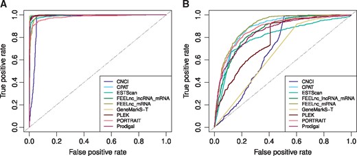
The ROC curves demonstrating the performances of the RNA classification tools on the two human test sets. (A) Mix with human transcripts and (B) mix with shuffled sequences.
Among all the tools, the best performance in terms of average MCC/AUC on the four test sets were observed for FEELnc (‘mRNA + lncRNA’ mode: average MCC = 0.779/average AUC = 0.944, ‘mRNA + shuffle’ mode: 0.754/0.955) and CPAT (0.773/0.943). In most cases, these tools demonstrated similar performances. FEELnc clearly outperformed CPAT in terms of pAUC values on the mouse short-CDS test set only (Supplementary Figure S6D). Interestingly, on the long CDS test sets FEELnc (mRNA + lncRNA) outperformed FEELnc (mRNA + shuffle), while the situation was opposite on the short-CDS test sets. This observation may indicate that the FEELnc performance in the mRNA + lncRNA training mode largely depends on the provided training sequences. As expected, the tools performed better on the long-CDS than on the short-CDS test sets (the average MCC value for all the tools decreased from 0.822 to 0.509, while the average AUC value decreased from 0.988 to 0.814).
The self-training tools (GeneMarkS-T and Prodigal) were of the special interest in our study, as they do not rely on the pre-built models and do not require training sets. Therefore, such tools could be applied to non-model organisms with poor annotation available. GeneMarkS-T outperformed Prodigal according to the average MCC (0.624 versus 0.332) but not average AUC (0.843 versus 0.924) values. Yet, self-training algorithms concede to the tools with an incorporated gene model. Alternatively, a pre-built ‘universal’ model of PORTRAIT can also be applied to non-model species. On average, PORTRAIT outperformed self-training tools (the average MCC/AUC = 0.728/0.929), especially on the sequences with short CDS.
Thus, our analysis indicated that FEELnc is a good tool for ab initio RNA classification if a reliable species-specific training set of mRNA and/or lncRNA sequences is available. CPAT seems to be a good alternative with pre-built models for several vertebrate species. PORTAIT and GeneMarkS-T can be advised for the analysis of RNAs from non-model organisms. Taking into account that even the best tool may perform less impressive on a specific set, our advice is to consider predictions from several computational approaches to make sure that a transcript in question is indeed noncoding.
Benchmarking the RNA-RNA interaction prediction tools
To assess the performance of the existing RNA-RNA interaction prediction tools on mammalian transcripts, three types of test sets were made based on the available experimental data. These test sets addressed different modes of analyzing intermolecular interactions—‘one-vs-one’, ‘one-vs-many’ and ‘many-vs-many’ (Figure 2A).
First, we investigated the ‘one-vs-one’ search type. We expected that for the experimentally validated interactions, the predicted binding between the original transcript sequences should be stronger than between the shuffled sequences. For this purpose, we collected 17 functional pairs of mammalian long RNAs with experimentally proven hybridizations (Supplementary Table S1). Empirical P-values were computed for all the transcript pairs based on the output of each RNA-RNA interaction prediction tool (Supplementary Table S3). Among all the tested tools, RIblast, LncTar and IRIS had the least number of false-negative errors (defined as functional RNA-RNA interactions with empirical P-value > 0.05, Table 5).
Comparison of the RNA-RNA interaction prediction approaches on four test sets.
| 17 RNA-RNA pairs | TINCR RIA-seq | SPLASH: top 50 RNAs | |||||||||
|---|---|---|---|---|---|---|---|---|---|---|---|
| Mix with human | Mix with shuffled | ||||||||||
| Time | Errors | Time | AUC | pAUC | Time | AUC | pAUC | Time | AUC | pAUC | |
| GUUGle | 44 | 5 | 44 | 0.507 | 0.0039 | 45 | 0.602 | 0.0146 | 28 | 0.56 | 0.007 |
| BLASTn | 248 | 5 | 224 | 0.458 | 0.0058 | 210 | 0.558 | 0.0089 | 424 | 0.555 | 0.0087 |
| RIsearch2 | 316 | 4 | 892 | 0.501 | 0.0036 | 902 | 0.551 | 0.0062 | 859 | 0.52 | 0.0068 |
| LASTAL | 392 | 5 | 1950 | 0.521 | 0.007 | 1920 | 0.711 | 0.0208 | 1014 | 0.528 | 0.0093 |
| DuplexFold | 2967 | 6 | 11 155 | 0.496 | 0.005 | 8770 | 0.47 | 0.0036 | 5202 | 0.518 | 0.0077 |
| RNAplex-c | 4599 | 6 | 9855 | 0.479 | 0.0018 | 8079 | 0.551 | 0.0013 | 3053 | 0.45 | 0.0046 |
| RNAplex-a | 6527 | 7 | 6703 | 0.509 | 0.0051 | 6706 | 0.597 | 0.0132 | 4716 | 0.55 | 0.0055 |
| RIblast | 7305 | 3 | 5770 | 0.548 | 0.0075 | 5600 | 0.711 | 0.0268 | 17 715 | 0.521 | 0.005 |
| ASSA | 10 280 | 4 | 44 746 | 0.557 | 0.0045 | 30 522 | 0.858 | 0.0461 | 11 868 | 0.564 | 0.0057 |
| RRP | 16 493 | 5 | 10 010 | 0.497 | 0.0044 | 9760 | 0.577 | 0.0124 | 42 319 | 0.529 | 0.0077 |
| RNAduplex | 17 216 | 7 | 40 711 | 0.492 | 0.0046 | 34 116 | 0.482 | 0.0036 | 12 358 | 0.522 | 0.0079 |
| LncTar | 18 117 | 3 | 29 110 | 0.481 | 0.0041 | 29 682 | 0.535 | 0.0055 | 24 026 | 0.454 | 0.0031 |
| IRIS | 56 906 | 3 | 121 983 | 0.494 | 0.0051 | 120 062 | 0.51 | 0.0056 | 73 338 | 0.537 | 0.0075 |
| IntaRNA2 | 219 662 | 4 | – | – | – | – | – | – | – | – | – |
| RactIP | 593 028 | 8 | – | – | – | – | – | – | – | – | – |
| RNAup | 651 544 | 4 | – | – | – | – | – | – | – | – | – |
| AccessFold | 3 397 428 | 5 | – | – | – | – | – | – | – | – | – |
| Bifold | 4 541 429 | 5 | – | – | – | – | – | – | – | – | – |
Note: The tools are sorted by the execution time on the ‘17 RNA-RNA pairs’ test set. The five slowest tools were not applied to the large-scale test sets because of the execution time restrictions. Column notation: Time—total execution time on the corresponding test set (in seconds), errors—the number of false-negative errors (true RNA-RNA pairs that do not pass the 0.05 threshold on the empirical P-value), AUC—area under the ROC curve, pAUC—partial AUC (false-positive rate range between 0 and 0.1). The best value in each comparison column is highlighted in bold.
The ‘one-vs-one’ analysis demonstrated that detection of the short-trans interactions appeared to be the most difficult task for all the tools (Supplementary Table S3). On the other hand, experimental data indicate that interactions of this type are likely to be the most frequent in mammalian cells [95, 96]. For example, the RNA interactome analysis (RIA-seq) experiment demonstrated that in human keratinocytes TINCR binds to transcripts corresponding to 1814 unique genes. It should be noted that TINCR transcript (NR_027064) contains an Alu repeat in the ‘+’ orientation and can potentially form Alu-based duplexes with other RNAs [97]. However, only a small fraction of TINCR-associated transcripts (12%) have Alu’s in ‘–‘ orientation suggesting that the majority of the TINCR interactions are not repeat-based.
Therefore, we focused the benchmarking of the ‘one-vs-all’ search on predicting short-trans interactions by compiling two test sets of Alu-free sequences. The fastest tools were used to search for TINCR partners in the two test sets of 1000 sequences each. ROC curves were build based on the obtained predictions, and the corresponding statistics (AUC and pAUC) were computed (Figure 4 and Supplementary Figure S7). For the ‘mix with human transcripts’ data set top three performing tools (ASSA, RIblast and LASTAL) produced AUC values of 0.557, 0.548 and 0.521, respectively, which is only slightly above the one produced by a random classifier (AUC = 0.5) (Table 5 and Figure 4A). This indicates that most of the tools could not efficiently distinguish true TINCR targets from other human transcripts. Yet, the performances of almost all the tools improved on the ‘mix with shuffled sequences’ test set (Figure 4B). ASSA outperformed all other approaches in terms of AUC and pAUC values on this test set.
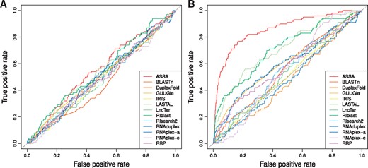
The ROC curves demonstrating the performances of the RNA-RNA interaction prediction tools on the two TINCR test sets. (A) MEG3 test set and (B) MEG3 genome-wide predictions.
Finally, in some cases, one may be interested in identifying all RNA-RNA interactions within a given set of RNAs. This can be done by performing the ‘all-vs-all’ (or ‘many-vs-many’) search type. We investigated the ability of different computational tools to reconstruct the network of intermolecular base-pairing between long RNAs that has been experimentally identified by the SPLASH method [94]. Our test set consisted of 50 transcripts (mRNAs and lncRNAs only) that formed 276 interacting pairs (Figure 2A). Each tool was used to perform all-vs-all search, and all the unique transcript pairs (1225 in total) were ranked according to the predicted strength. The observed performances of the tools resembled the results obtained for the ‘TINCR mix with human transcripts’ test set (Supplementary Figure S8). The best AUC and pAUC values were produced by ASSA (0.564) and LASTAL (0.0093), respectively (Table 5). To conclude, our results indicate that computational prediction of RNA-RNA interactions between long sequences, especially on the level of complete transcriptome, remains a challenging task.
Benchmarking the RNA-DNA triplex prediction tools
For our benchmarking, we used two tools currently available for RNA-DNA triplex prediction: LongTarget and Triplexator. First, we applied the tools to the seven cases of triplex-based interactions manually collected from literature (Supplementary Table S2). Only Triplexator in the default (‘all motifs’) mode was able to classify all seven known interactions as statistically significant (empirical P-value ¡ 0.05, Table 6). Interestingly, analysis of the errors, which appeared if a restricted set of the Triplexator rules was used (the -m option), allowed to make preliminary conclusions about the underlying hybridization motifs. For example, interactions between lncRNA Fendrr with both of its targets were predicted for the ‘-m P’ (parallel, Hoogsteen bonds) and ‘-m Y’ (pyrimidine, C and T) settings only (Supplementary Table S4). Indeed, Fendrr targets (GGA)n repeats located in the promoters of both target genes and the corresponding Hoogsteen bonds C::G and T::A require pyrimidines in the RNA.
Comparison of the RNA-DNA triplex prediction approaches on two test sets.
| 7 lncRNA-DNA pairs | MEG3 ChOP-seq test set | ||||
|---|---|---|---|---|---|
| Time | Errors | Time | AUC | pAUC | |
| LongTarget | 180245 | 2 | 126818 | 0.54 | 0.0064 |
| Triplexator (default) | 7 | 0 | 61 | 0.612 | 0.0179 |
| Triplexator (-m A) | 6 | 2 | 30 | 0.607 | 0.0179 |
| Triplexator (-m M) | 7 | 3 | 29 | 0.59 | 0.0171 |
| Triplexator (-m P) | 6 | 1 | 41 | 0.593 | 0.0146 |
| Triplexator (-m R) | 6 | 3 | 20 | 0.58 | 0.0169 |
| Triplexator (-m Y) | 6 | 3 | 32 | 0.579 | 0.0136 |
Note: Column notation: Time—total execution time on the corresponding test set (in seconds), AUC—area under the ROC curve, pAUC—partial AUC (false-positive rate range between 0 and 0.1). The best value in each comparison column is highlighted in bold.
Next, we tested the ability of the tools to identify triplex-based RNA-DNA interactions on the genome scale using ChOP-seq data on MEG3 interactions with chromatin. We used both tools to predict the interaction strengths between the MEG3 transcript (NR_002766) and 700 genomic regions containing MEG3 binding sites and 1400 regions without MEG3 binding sites (Figure 2B). ROC curves (Figure 5A and Supplementary Figure S9) showed that Triplexator with the default settings produced the best results (AUC = 0.612, Table 6). Moreover, Triplexator with any restricted rule set outperformed LongTarget. Interestingly, Triplexator performance did not drop significantly when restrictions on the base pairing motifs were applied. This fact may indicate that MEG3 uses several different Hoogsteen rules to bind to DNA rather than following a specific rule as in the case of Fendrr.
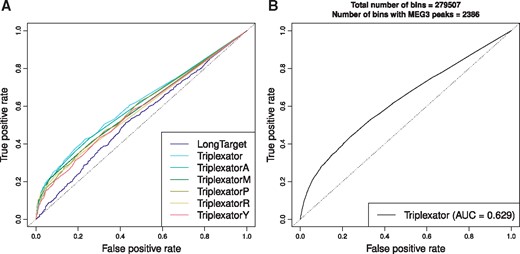
The ROC curves demonstrating (A) the performances of the RNA-DNA triplex prediction approaches on a subset of the MEG3 peaks and (B) the Triplexator performance on the genome-wide search (279 507 genomic regions in total).
It should also be noted that in this test set, we applied the tools to a subset of MEG3-bound regions because of the large running time of the LongTarget. Triplexator turned out to be not only the most accurate tool in our tests but it also worked much faster than LongTarget. Its embedded ability for parallel calculations makes Triplexator a suitable tool for large-scale (e.g. genome-wide) computations. Indeed, we were able to predict interactions between MEG3 and all genomic regions and obtained a similar AUC value (0.629, Figure 5B).
In terms of usability, Triplexator is more flexible: some of the base-pairing rules can be excluded by the users, while with LongTarget users can only penalize TT or CC stretches. Also, Triplexator can treat differently mismatches in the core of the triplex as compared to its end, which may reflect the stability of binding. Although for the benchmark we used default or recommended settings, the flexibility of settings can be beneficial in practice. In summary, Triplexator clearly outperformed LongTarget in both accuracy of prediction and usability.
Discussion
In this benchmarking study, we compared computational methods for lncRNA classification and analysis of their possible interactions. Our work was inspired by the discovery and increasing evidence of functionality of thousands of noncoding transcripts in mammalian cells. Thus, where possible, we attempted to use lncRNA-related experimental data. Clearly, it is not possible to cover all computational problems related to lncRNA functionality. So, we focused on transcript classification into protein-coding and noncoding RNAs, as well as on prediction of intermolecular RNA-RNA hybridization and triplex-based RNA-DNA binding. To make our conclusions more reliable, we applied every computational tool to at least two independent test sets and computed several statistics (MCC, AUC and, in special cases, the number of FN predictions by computing empirical P-values).
Four test sets were used for benchmarking the tools that classify transcripts into protein-coding and noncoding. Most of the tools demonstrated similar performance on the human and mouse transcripts. Still for all the tools distinguishing short-CDS mRNAs from lncRNAs was a more challenging task. Nevertheless, even in this case, the best tools produced AUC values above 90%.
In contrast, performances of the RNA-RNA and RNA-DNA interaction prediction tools were not good. The prediction of the MEG3 target sites on the genome scale by the best tool Triplexator had AUC value just around 60%. Performance of the RNA-RNA prediction tools on the test sets that resembled real-life situations (i.e. did not include random sequences) was even worse—the best performance did not exceed 57%. Such poor prediction may at least partially be a consequence of a non-direct interaction detected by the experimental procedures and may also reflect the complexity of the studied system. It should be noted that on the RNA-RNA interaction test set where the false targets were represented by shuffled sequences ASSA demonstrated performance above 85%. Unfortunately, such test has less resemblance with the real life tasks and may not be useful to reveal the function and the mechanism of action of a real lncRNAs.
Large-scale search results (i.e. ‘one-vs-many’ and ‘many-vs-many’ test sets) produced by ASSA were the most accurate among all the tools. This tool not only takes RNA secondary structure into account but also provides a statistical significance estimate (P-value) for every predicted interaction energy. It should be noted that ASSA P-values are computed with respect to the lengths and GC contents of the input sequences. This provides automatic correction to the properties of the input transcripts and makes various predictions comparable with each other, which is important for the whole transcriptome screening. On the other hand, all the other thermodynamics based tools compute interaction energy for each RNA pair. We observed that the ΔG or SumEnergy values increased with the sequence length (Supplementary Figure S10A–D). Therefore, some of the short true targets cannot appear on top of the prediction list because stronger binding will usually be predicted for the longer sequences. It should be noted that LncTar also addresses this problem by computing normalized ΔG values (ndG). Still, this tool has a poor performance on both TINCR test sets. There may be an issue with the ΔG normalization because we observed opposite trend for ndG values—they decrease with the sequence length (Supplementary Figure S10H). Additional tuning of the ndG calculation may improve performance of this tool.
Our analysis of the RNA-DNA triplex prediction demonstrated that the usage of additional triplex forming rules by LongTarget did not improve the prediction accuracy. Probably, such base-pairing happens rare in real triplexes; therefore, usage of these rules does not increase sensitivity enough to compensate for the reduced specificity. We believe that estimate of a statistical significance of a detected triplex based on the number of triplexes detected in the shuffled RNA/DNA sequence, proposed by authors of LongTarget, may improve the prediction accuracy. Yet, single-nucleotide shuffling may overestimate that the significance of a detected triplex, dinucleotide or trinucleotide shuffling should provide more reliable estimate. Also, none of the triplex predicting tools incorporate RNA secondary structure in the model, which may lead to prediction of a triplex forming oligonucleotide (TFO) and a triplex in the non-accessible RNA region.
It should be noted that the default settings were used to run the tools included in this study. It is possible that tuning the parameters of the algorithms may improve their performance on a particular data set. At the same time, it may lead to over-fitting, and it is unlikely that such tuned model can be used for a different data set. This is why in this benchmark we did not optimize algorithm parameters to perform better on a specific data set reporting the ‘out-of-the-box’ performance of the tools.
Additionally, a special preprocessing or filtering of the raw data (e.g. by considering highly expressed genes or open chromatin regions only) may also increase the accuracy of the bioinformatics predictions. However, such approaches depend on the availability of the specific experimental data and will require additional time and effort from the potential users of the tools. The currently available experimentally validated data sets on RNA-RNA and RNA-DNA interactions are limited and possibly biased. Further development of the experimental techniques will contribute to a better training set for computational models.
The tasks described in our study can be directly approached by various experimental methods. Namely, one can perform a large-scale proteomics study or analyze a number of publicly available data from various cell types to make sure that the RNA of interest is not translated and can be classified as ‘non-coding’. A significant progress has been made in a large-scale identification of intermolecular RNA-RNA interactions in living cells. Such methods as RIA-seq allow to uncover all partners of one RNA in a given cell type [40]. Recently, several new experimental techniques (SPLASH [94], PARIS [95], LIGR-seq [96], MARIO [98]) have been used to identify intermolecular interactions between all RNAs expressed in a particular cell type. Finally, several methods (ChIRP-seq [34], MARGI [99], ChAR-seq [100], GRID-seq [101]) can map RNA-chromatin binding on the whole-genome scale. Analysis of the experimental data produced by these methods identifies the whole lncRNA interactomes. Nevertheless, it remains unclear whether the observed binding is direct (RNA-RNA/RNA-DNA hybridization) or indirect (e.g. mediated by the RNA- or DNA-binding proteins). Additionally, such experimental data may be biased to detect interaction for the highly expressed genes only. Therefore, further development of the bioinformatics tools predicting specific binding mechanisms remains an important task. Additionally, computational predictions can be easily obtained for a number of species, opening the possibility to study evolution of a particular lncRNA and its interactions. Summing up, we should state that computational prediction of RNA interactions, especially at the level of whole-genome/transcriptome, presents a significant challenge; yet, this important problem has to be solved to increase our knowledge of lncRNA biology.
Conclusions and further directions
Our benchmark shows that with the availability of complete transcriptomes, the task of distinguishing between mRNA and lncRNA (at least for the antisense and lincRNA types) can be solved with relatively high accuracy. Yet, the classification of RNAs with short CDS remains challenging even for the best performing tools. The remaining problem is to determine if a particular protein-coding RNA has an additional nonprotein-coding function. The computational tools to search for such RNAs are yet to be developed.
We also demonstrate that prediction of RNA-RNA and RNA-DNA interactions on the scale of the complete transcriptome and genome is not a trivial task. The most challenging part of this problem is the prediction of short-trans interactions. All programs designed for solving this task basically failed. Our results suggest that the normalization of the predicted RNA-RNA interaction strength to the transcript length and GC content may improve the prediction accuracy. There is still a lot of room for improvement of the methods to predict interactions of RNA with other nucleic acids.
FEELnc and CPAT are the best tools to distinguish between coding and noncoding mammalian transcripts (both tools have average AUC value > 94%).
For non-model organisms, GeneMarkS-T and PORTRAIT provide a decent alternative (average AUC value > 84%)
Large-scale prediction of RNA-RNA and RNA-DNA interactions remains a challenging task with the best average AUC values at 56% (ASSA, RIBlast and LASTAL) and at 61% (Triplexator), respectively.
Normalization of the predicted interaction strength to the transcript length and GC content as well as statistical significance estimates may improve the RNA-RNA and RNA-DNA prediction accuracy.
Short-trans RNA-RNA and RNA-DNA interactions are predicted poorly at this stage.
Acknowledgements
The authors would like to thank Dr Yue Wan for providing human transcript sequences for the all-vs-all RNA-RNA search.
Funding
The RNA-RNA interaction prediction has been supported by the Dynasty foundation (Postdoctoral Fellowship No DP-B- 26/14 to I.A.). The RNA classification and RNA-DNA interaction prediction has been supported by RSF 15-14-30002 to Y.A.M.
Ivan V. Antonov is a postdoctoral research scientist at the Research Center of Biotechnology RAS, Moscow. His research interests include long noncoding RNAs, RNA-RNA interactions, post-transcriptional and epigenetic gene regulation as well as programmed frameshifting.
Evgeny Mazurov is a programmer and a student at the School of Bioinformatics.
Mark Borodovsky research interests are in developing algorithms for genome structural annotation. Several algorithms developed in previous years have been used in a number of genome sequencing projects. Dr Borodovsky is a Founder of the Georgia Tech graduate program in Bioinformatics.
Yulia A. Medvedeva works in the area of regulatory genomics, transcriptomics and epigenomics. Her main interests include the role of lncRNA, DNA methylation and histone modifications in regulation of genome stability and transcription.
