


Abstract
Heterophylly, i.e. morphological changes in leaves along the axis of an individual plant, is regarded as a strategy used by plants to cope with environmental change. However, little is known of the extent to which heterophylly is controlled by genes and how each underlying gene exerts its effect on heterophyllous variation. We described a geometric morphometric model that can quantify heterophylly in plants and further constructed an R-based computing platform by integrating this model into a genetic mapping and association setting. The platform, named HpQTL, allows specific quantitative trait loci mediating heterophyllous variation to be mapped throughout the genome. The statistical properties of HpQTL were examined and validated via computer simulation. Its biological relevance was demonstrated by results from a real data analysis of heterophylly in a wood plant, mei (Prunus mume). HpQTL provides a powerful tool to analyze heterophylly and its underlying genetic architecture in a quantitative manner. It also contributes a new approach for genome-wide association studies aimed to dissect the programmed regulation of plant development and evolution.
Introduction
The shoot of a plant grows by adding new metamers at its apex that form internodes, leaves and buds. These shoot components display gradual or disrupt transitions along the shoot, even in a constant environment, a phenomenon observed pervasively in most land plants [1–4]. Shape variation in leaves produced on the same shoot, particularly called heterophylly, is a concept that has received a great deal of attention during the past centuries [5–10]. It has been widely accepted that heterophylly is of ecological and evolutionary significance because it is adaptive and functional under particular environmental conditions [8, 11, 12]. Heterophyllous characteristics have well been described from morphological, anatomical and physiological aspects [13, 14]. Several studies have revealed the biochemical mechanisms underlying heterophylly, identifying various hormones, such as ethylene and abscisic acid (ABA), involved in the sequential alteration of leaf form [15, 16].
More recently, many studies have begun to characterize the mechanistic link between gene expression, hormonal action and heterophylly [4, 17]. It has been observed that KNOTTED1-like homeobox orthologs participate in regulating heterophyllous expression for Rorippa aquatica (Brassicaceae), through the accumulation of gibberellin in the leaf primordia [17]. In the aquatic fern Marsilea quadrifolia, plant hormone ABA-responsive heterophylly genes were identified, showing diverse patterns of expression during heterophyllous induction [18]. The transcriptomic analysis of RNA-seq data identified the key role of SQUAMOSA promoter-binding protein like, NAC and YUCCA genes in the heterophyllous variation of Gevuina avellana, a temperate rainforest tree [19]. Despite extensive efforts to link gene expression with heterophylly, however, little is known about the genetic architecture of heterophyllous variation, including the number of genes involved, their genomic locations and the magnitudes of their genetic effects.
Genetic mapping or association studies built on artificial or natural populations provide a powerful tool to dissect the genetic control of heterophylly and relate this knowledge with the environmental adaptation of plants. To perform genetic mapping, heterrophylly is treated as a phenotypic trait that is defined quantitatively. Traditional approaches for defining leaf shape are based on the measurements of leaf traits, such as length, width, angle and ratio of length to width, analyzed by multivariate morphometric methods [20, 21], but these approaches are not precise, as they contain little information about the spatial distribution of shape change. As a result of this drawback, geometric morphometrics (GM) that can precisely characterize shape variation has arisen as a useful approach for shape analysis in the past two decades [22, 23]. Two GM approaches based on landmarks and outlines have been developed [24, 25] and, more recently, integrated into genetic mapping, aimed to map specific shape quantitative trait loci (QTLs) for a variety of organs [26–28].
Current models for shape mapping were designed to characterize shape variation on a single position of organisms at a time, but fail to capture the differentiation of organ shape on multiple positions, such as heterophylly, limiting their applications to addressing more complex biological questions. The motivations of this article are to expand the principle of GM-based shape mapping to map QTLs for multiple shapes and detail a statistical procedure of testing how a shape QTL contributes to heterophyllous variation within a plant. The statistical method was packed as an R platform, allowing the new method to be used freely by other researchers interested in studying the genetic architecture of heterophylly. The new method was applied to analyze mapping data of heterophylly in a woody plant, mei (Prunus mume), leading to the identification of key QTLs correlated with the capacity of plants to alter their leaf shape in response to environmental perturbations.
Model
Genetic design
A segregating population is prerequisite for mapping QTLs. Consider a mapping population that contains n plants all genotyped for a panel of molecular markers throughout the genome. Different from traditional strategies that measure and map a single phenotype, the new model allows high-dimensional phenotypic data to be mapped at the same time. Assume that J leaves, labeled as 1, … , J in order from bottom to top, located along the axis of a shoot are photoed for each plant. The contour of each leaf is delineated by choosing a finite number of semilandmarks (say L) on its boundary. These semilandmarks are spaced clockwise at equally spaced radii, having each point described by x and y coordinates, representing the shape of a leaf. Let t0, t1, … , tL denote the accumulated length of step segments from semilandmark 1, … , L, respectively.
Fourier modeling of the mean vectors
The shapes of all leaves from the same metamer on a shoot need to be aligned among different plants, to minimize variation caused by position, scale and rotation [32]. However, as heterophylly contains within-plant variation not only in leaf shape but also in leaf size, a Procrustes alignment is made for outlines of leaves from different metamers on the same shoot, by adjusting for variation only because of position and rotation but not because of scale. Giardina and Kuhl [33] proposed a direct procedure for normalizing the EF analysis coefficients calculated from raw outlines to remove the position and rotation effects. This procedure that was integrated into Bo et al.’s shape mapping can be used directly in the current model for mapping heterophylly.
Autoregressive modeling of the covariance matrix
Taken together, model parameters contained in Equations (10a–)–(10c), arrayed in η, were used to model the structure of residual covariance matrices for x- and y-coordinates. Based on such structural modeling, the closed forms of the determinants and inverses for the residual matrix, , can be derived. By implementing these closed forms into the solving procedure of likelihood (1), the computational efficient of residual covariance matrices can be enhanced.
Hypothesis tests
Under the null hypothesis, genotype-specific EF parameters can be estimated with the implementation of the EM algorithm with constraints.
Different components of Fourier series show different properties of leaf shape. The sine components in Equations (4a) and (4b) are related with the asymmetry of a leaf, whereas the cosine components are related with the symmetry of a leaf. Thus, by testing these two components separately, we can examine how a QTL affects the symmetry and asymmetry of a leaf.
We implemented the model of mapping heterophylly into an R-based platform, HpQTL, for its broad use by other interesting researchers. The package lists several functions for shape QTL mapping, including shape alignment and digitizing, EF curve fitting and QTL mapping.
A worked example
Plant material
The biological usefulness of the new model was validated by analyzing a mapping data about heterophylly in mei (P. mume), a woody plant species. By crossing two cultivars, P. mume ‘Fenban’ (BJFU1210120013) as the female parent and P. mume ‘Kouzi Yudie’ (BJFU1210120022) as the male parent, both from Qingdao Mei Garden, Qingdao, China, we obtained a segregating F1 population of 228 progeny [35, 36]. The population was genotyped for 1484 SNP markers and InDels. For a full-sib family derived from two heterozygous parents, a marker may be segregating according to either F2-like intercross or backcross-like testcross [37–39]. The markers genotyped include 271 intercross markers and 1213 testcross markers. Of these testcross markers, 620 and 593 are segregating because of the heterozygosity of parents Fenban and Kouzi Yudie, respectively. JoinMap version 4 [40] was used to construct a genetic linkage map from SSR and SNP markers. The map is composed of eight linkage groups corresponding to mei’s eight haploid chromosomes. The total length of the map is 670 cm, with an average marker distance of 0.5 cm.
All the F1 hybrids and their parents were grown in the Xiao Tangshan Horticultural Trial, Beijing, China [35, 36]. All F1 hybrids were cut off after 1 year of growth in the field. In the next spring, new shoots sprouted from 1 year rooting systems. During the end of July, the fast-growing season of mei, we chose three equally spaced leaves on the main stem to study the genetic control of heterophylly in woody plants. The shape of the three chosen leaves was measured by their digital images. The two parents, Fenban (female) and Kouzi Yudie (male), differ in leaf shape, with former having a more rounded leaf blade while the latter having a longer tip (Figure 1) The F1 genotypes derived from these two parents display considerable variation in leaf shape.
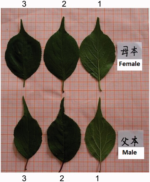
Differences in leaf shape between two parents, Fenban (female parent) and Kouzi Yudie (male parent), used to generate an F1 full-sib family. Three leaves, labeled as 1, 2 and 3, from the shoot tip, were sampled to show heterophylly.
Mapping heterophylly QTLs
The R package implementing the new mapping model, i.e HpQTL, was used to analyze the heterophylly data of mei. Leaf image data were loaded in R, from which to discern the object and background and translate the images to black and white based on 600 × 900 pixels from a leaf digital image (Figure 2). Next, we marked a set of semilandmarks on the boundary of each leaf spaced at an equal radial angle (Figure 2) and get the coordinates of each point in a two-dimensional matrix, from which we can obtain the shape of each leaf in terms of x- and y-coordinates. It can be seen that there is great variability in x- and y-coordinates among the F1 hybrids, which can be compared with the difference in leaf shape between the two parents.
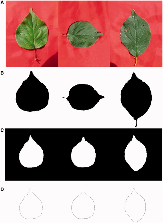
The procedure of extracting leaf boundary from a leaf image. (A) Original color images. (B) Black and white images translated from color images. (C) Shape alignment by filtering out the position, scale and rotation effects. (D) A set of points on the boundary spaced at an equal radial angle.
Normalized EF analysis aimed to remove the position and rotation effects of raw outlines [33] was used to fit curves to the outlines of leaf shape. The goodness-of-fit of the original data to normalized outlines depends on the choice of the number of harmonics in contour analysis. An optimal number of harmonics were determined by information criterion AIC. AIC suggests that four is an optimal number of harmonics, with the first four harmonics explaining nearly 95% of leaf shape information (Figure 3). The estimates of EF coefficients under the first nine harmonics are given in Supplementary Table S1. By reading marker data, we used HpQTL to perform QTL mapping for heterophylly described by Fourier functions, obtaining a plot of log-likelihood ratio values that reflect the significance of marker associations over the genome. Through a multiple comparison, we identified five significant QTLs associated with heterophyllous variation (Figure 4).
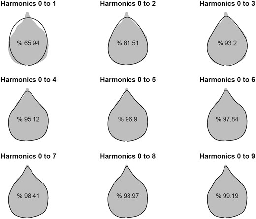
Outline reconstruction from EF analysis applied to the outline coordinates of a random leaf. The original outline corresponds to the gray shape, while reconstructed leaves are solid black outlines. The percentage of an actual leaf shape explained by the reconstructed shape, as seen in the leaf shape, increases with the harmonic order of EF function.

The genetic map locations of QTLs that control Fourier parameters throughout eight linkage groups of the P. mume genome. The cases for testcross markers and intercross markers are given, respectively, because they have different critical thresholds (15.0 for testcross markers and 14.8 for intercross markers at a marginal significance level) determined from permutation tests.
To show how a QTL controls heterophylly, we picked up the most significant QTL hk_hk1742 on chromosome 2 to explain its spatial pattern of genetic effect. Three genotypes of this QTL well explain the variation of leaf shape from each of three positions among F1 hybrids in terms of x- and y-coordinate values (Figure 5). By translating EF curves back to leaf shape, we can visualize in which part of leaf shape the three genotypes differ. For example, for the top leaf (Leaf 1), two homozygotes tend to be similar to each another, but both of which are different dramatically from the heterozygote. The heterozygote is relatively more ovate than the homozygotes.
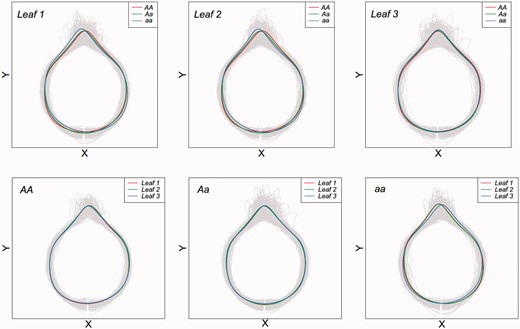
Visualized variation in the shape of three heterophyllous leaves in P. mume at an intercross QTL of the largest test statistic (hk_hk1742 on chromosome 2). The upper panel shows genotypic variation among three genotypes AA, Aa and aa for each leaf, whereas the lower panel shows heterophyllous variation for each genotype.
It is interesting to note that this QTL affects leaf shape in different ways depending on where a leaf is located on the main stem. Overall, the QTL displays an increased effect on leaf shape with an increasing leaf position according to hypothesis tests (11) (Figure 5), which suggests that this is a heterophyllous QTL.<AQ5/> Of three genotypes, the two homozygotes tend to be stable over different positions, but the heterozygote alters its leaf shape strikingly from the bottom to top. This result suggests that the dominant effect of this QTL produces an important role in regulating the heterophylly of mei trees.
Computer simulation
HpQTL was equipped with a functionality to perform Monte Carlo simulation studies which test the statistical power of the model and the precision of its parameter estimation. Here, we present an example to show the statistical property of HpQTL. The simulation mimicked the working example of mei, assuming a segregating population of 250 individuals in which a QTL exists to affect heterophylly. For each genotype of the QTL, we hypothesized a set of EF parameters from a Fourier series function with four harmonics for three heterophyllous leaves located on the same shoot. The phenotypic values of x- and y-coordinates for these three leaves were simulated by genotypic values of the QTL plus residual errors whose covariance structure follow the antedependence model.
Supplementary Table S2 gives the results about the maximum likelihood estimates of genotype-specific EE parameters from the assumed mapping population under 0.1 heritability of heterophylly. Overall, HpQTL provides reasonably accurate and precise estimates of all Fourier parameters for three heterophyllous leaves at different QTLs genotypes. By using these estimated parameters, we reconstructed the shape of each leaf at a different shoot position for the three genotypes (Figure 6). All leaf shapes can be well estimated, suggesting the statistical efficacy of HpQTL. We conducted an additional simulation study to investigate the power of heterophylly QTL detection by simulating the phenotypic data of a mapping population of 250 individuals containing a single group. It was found that the empirical power of QTL detection by HpQTL is beyond 0.95. Also, HpQTL can well estimate the genetic effect of the QTL on the heterophyllous differentiation of leaf shape among different shoot positions.
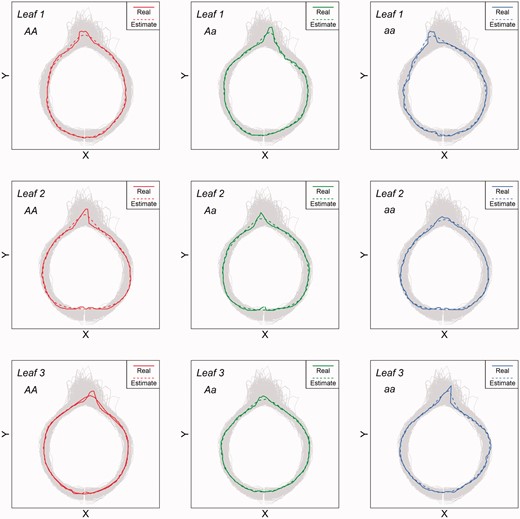
Comparison of estimated leaf shape with actual leaf shape for different genotypes and different heterophyllous leaves from simulated data.
Discussion
A central question in developmental biology is how cells and tissues properly alter their performances over time to best adapt to endogenous and exogenous environments. One of the most pronounced examples of this phenomenon in plants is heterophylly that involves the transition of leaf size and shape from one position to next on the same shoot [11]. How heterophylly takes place, how it plays a role in ecological and evolutionary processes and, more importantly, what is its genetic signature have been an interesting subject of attention for centuries, and these questions have continued to intrigue modern biologists [5–10].
This study presented a quantitative description of heterophylly by implementing GM, overcoming the inaccuracy of traditional shape analysis purely relying on length, width, angle and ratio [32]. Although heterophyllous plants offer fascinating opportunities to study developmental questions related to plant adaptation and speciation, the previous description of heterophyllous changes in plants has developed in an inconsistent way, which prevents the extraction of useful information from this phenomenon. The GM-based approach developed can precisely characterize the subtle variation of leaf morphologies and their developmental changes over time and space. First, it quantifies the outline of leaf shape by fitting EF functions [29–31] and uses EF parameters to capture the origin and sources of shape variation. In plants, the place of leaves that exhibit phenotypic variation may be related to the plant’s capacity to respond to light irradiation. For example, more ovate leaves are thought to be able to capture more light than more lanceolate leaves [9]; thus, the detailed characterization of shape variation in different positions is of use to address key ecological questions in plants.
Second, we implemented EF functions into a genetic mapping or association study framework, allowing the underlying genetic control by individual QTLs to be characterized. This implementation leads to a so-called HpQTL R platform, which has multiple functionalities. It can test whether there is specific QTL that controls heterophylly in plant, followed by a testing procedure of how the QTL regulates heterophyllous change and how each QTL genotype changes its expression of leaf shape from the bottom to up position in plants. HpQTL can help users to calculate the power of QTL detection, assess the precision of parameter estimation and determine the sample size optimally used for QTL detection.
HpQTL may be modified in several aspects. First, the model should be able to model the allometric relationship of leaf size and shape [9]. The current version identifies leaf shape variation that may be partly because of size by not adjusting for the scale effect. By calculating a position-varying single measure of leaf shape from x- and y-coordinates, we may draw a curve over leaf boundary. Thus, the area under curve (AUC) can be used to specify the size of a leaf. By mapping the AUC, we can judge how size QTLs are consistent with shape QTLs from which a network of pleiotropic control over leaf size and shape can be charted.
As heterophylly may be the consequence of plant adaptation, HpQTL should be modified to model the environmental components of heterophyllous variation. By planting the mapping population in multiple environments with recombinant inbred lines or clonal replicates [41], heterophylly and its environment-dependent variation can be characterized. The phenotypic changes of the same genotype over different environment can be termed environment-induced phenotypic plasticity (EiPH) [41–44], whereas the changes of the same phenotype within a plant, such as heterophylly, termed development-induced phenotypic plasticity (DiPH) [11]. The extended HpQTL model will not only characterize the genetic control of EiPH and DiPH, respectively, but also the pleiotropic control network of both of these features, better charting a comprehensive picture of the genetic architecture of heterophylly. HpQTL can be freely downloaded by other researchers at http://ccb.bjfu.edu.cn/program.html or can be requested from the corresponding author.
Key Points
Morphological variation in leaf size and shape within a single plant is termed heterophylly, regarded as the plant’s adaptation to surrounding environmental conditions.
The biochemical and molecular mechanisms underlying heterophyllic alteration have been investigated increasingly in the community of plant biological research.
Despite its fundamental importance, the genetic architecture of heterophyllous variation has not been systematically explored because of unavailability of the software that can precisely quantify within-plant variation in leaf shape.
We described and assessed a geometric morphometric approach for mapping QTLs that affect heterophyllous variation and packed this approach into an R-based platform for public use.
Supplementary Data
Supplementary data are available online at http://bib.oxfordjournals.org/.
Funding
The Beijing Nova program (grant number Z161100004916074), the Medium and Long Scientific Research Project for Young Teachers in Beijing Forestry University (grant number 2016ZCQ02), National Natural Science Foundation of China (grant number 31401900), Special Fund for Forest Scientific Research in the Public Welfare (grant number 201404102) and ‘One-thousand Person Plan’ Award.
Lidan Sun is a lecturer in Ornamental Genetics in Beijing Key Laboratory of Ornamental Plants Germplasm Innovation and Molecular Breeding, National Engineering Research Center for Floriculture at Beijing Forestry University.
Jing Wang is a doctoral student in Computational Genetics in the Center for Computational Biology at Beijing Forestry University.
Xuli Zhu is a doctoral student in Computational Genetics in the Center for Computational Biology at Beijing Forestry University.
Libo Jiang is a doctoral student in Computational Genetics in the Center for Computational Biology at Beijing Forestry University.
Kirk Gosik is a PhD candidate in Statistical Genetics in the Department of Public Health Sciences at Pennsylvania State University.
Mengmeng Sang is a doctoral student in Computational Genetics in the Center for Computational Biology at Beijing Forestry University.
Fengsuo Sun a doctoral student in Computational Genetics in the Center for Computational Biology at Beijing Forestry University.
Tangren Cheng is an associate professor of Ornamental Genetics and the executive director of National Engineering Research Center for Floriculture at Beijing Forestry University.
Qixiang Zhang is a professor of ornamental genetics and the director of National Engineering Research Center for Floriculture at Beijing Forestry University.
Rongling Wu founded the Center for Computational Biology at Beijing Forestry University. He is distinguished professor of Statistics and director of the Center for Statistical Genetics at Pennsylvania State University.
References
Author notes
These authors Lidan Sun, Jing Wang, Xuli Zhu and Libo Jiang contributed equally to this work.
