


Abstract
How trees allocate photosynthetic products to primary height growth and secondary radial growth reflects their capacity to best use environmental resources. Despite substantial efforts to explore tree height–diameter relationship empirically and through theoretical modeling, our understanding of the biological mechanisms that govern this phenomenon is still limited. By thinking of stem woody biomass production as an ecological system of apical and lateral growth components, we implement game theory to model and discern how these two components cooperate symbiotically with each other or compete for resources to determine the size of a tree stem. This resulting allometry game theory is further embedded within a genetic mapping and association paradigm, allowing the genetic loci mediating the carbon allocation of stemwood growth to be characterized and mapped throughout the genome. Allometry game theory was validated by analyzing a mapping data of stem height and diameter growth over perennial seasons in a poplar tree. Several key quantitative trait loci were found to interpret the process and pattern of stemwood growth through regulating the ecological interactions of stem apical and lateral growth. The application of allometry game theory enables the prediction of the situations in which the cooperation, competition or altruism is an optimal decision of a tree to fully use the environmental resources it owns.
Introduction
Wood biomass formation is a dynamic process involving interactions of primary height growth derived from the shoot apical meristem [1] and secondary radial growth from the vascular cambium [2]. The relationship between height and radial growth has been thought to be the ecological and evolutionary consequence of how trees adapt to their environment [3]. In nature, tree height is highly related to light capture [4], whereas stem circumference determines mechanical support [5, 6] and water transport efficiency [7]. The pattern of how height varies with diameter reflects a trade-off between growth and survival in a particular environment [8, 9]. Many forms of mathematical equations have been derived from engineering and biological design principles to describe such an allometric relationship of stem height and diameter [10, 11]. These equations have been widely applied to study the structural characteristic of forest trees to adapt to various environmental conditions [12–15] and predict the production of harvestable stem and carbon storage. Other studies also show the association of height–diameter allometry with wood structure, e.g. lignin and cellulose content [16–18].
The traditional allometric description can only evaluate the overall change of one trait as a function of the other, but does not provide insight into the internal mechanisms of how height growth affects diameter growth or vice versa. As a causal and sequential process, the allocation of resources to stem apical and lateral meristems depends heavily on growth conditions, such as spacing, biomechanical factors, site quality and age [15, 19, 20]. It is also clear that the causal relationship of stem height and diameter growth is determined by genetic factors [21, 22]. Key genetic mechanisms have been found to drive the allocation of carbon to apical and lateral growth; for example, several genes or proteins regulating the meristematic cells of the shoot tip also participate in the woody growth of the vascular cambium [23, 24]. A detailed understanding of how stem height and diameter interact with each other to determine woody biomass production and how this process is controlled by genes is a timely and necessary task to improve our knowledge of genetic processes underlying tree ecophysiology in changing climate.
Here, we argue that the implementation of game theory can reveal the ecological mechanism of stem woody growth dynamics in forest trees by quantifying the interaction and coordination of stem height and diameter growth. Despite the discrepancy of their underlying physiological mechanisms, the synergistic cooperation between stem height and radial growth can help trees’ success in survival, function and reproduction. However, when resources are short in supply, a greater growth rate in height or diameter may be attained at the cost of stem radial growth or height growth, respectively [19, 25]. Height growth and diameter growth thus form a trade-off relationship by competing for resources. Under the theory of Darwinian evolution, trees can decide which strategy, competition or cooperation they should use to maximize the function of the main stem in a given environment [26]. Equipped with a system of differential equations, game theory, originally developed in economic studies and extended to evolutionary biology [27–29], can be used to discern and quantify this strategy for trees.
Model
Game theory of stem allometry
Different strategies used by each trait will form six types of ecological interactions, i.e.
Mutualism, the two traits benefit from one another;
Synergism, no dramatic mutual benefit for both traits;
Competition, negative interactions between the two traits which may use the same pool of limited resources;
Commensalism, one trait benefits from another without being affected itself;
Predation/parasitism, one trait benefits at the cost of the other;
Amensalism, one trait harms the other despite no benefit for the former.
By estimating the interaction and scale parameters, we can quantify the degree of each possible interaction. While the interaction parameters determine whether and in which direction the dependent growth occurs, scale parameters, sH←D and sD←H, determine how the interaction strengthens or weakens with trait development. A positive or negative sH←D value implies that the interaction strengthens or weakens with the growth of stem diameter, respectively. If sH←D is zero, this means that the interaction does not depend on stem diameter growth. The same is true for sD←H.
Modeling framework of systems mapping
Systems mapping does not estimate individual elements in the mean vector (6) and covariance matrix (7), instead of model them using biologically and statistically relevant functions. Here, a system of ordinary differential equations (ODE) is implemented into the mean vector using a set of mathematical parameters Θj = (αHj, KHj, rHj, αDj, KDj, rDj; βH←Dj, sH←Dj, βD←Hj, sD←Hj), illustrating the temporal pattern of trait values for any specific QTL genotype j over time. Statistical algorithms for obtaining maximum likelihood estimates (MLEs) of genotype-specific ODE parameters and covariance-structuring parameters within the likelihood framework have been available. Fu et al. [38] implemented the fourth-order Runge–Kutt algorithm to estimate ODE parameters within a mixture-model setting. Ramsay et al. [39] proposed a generalized profiling approach for parameter estimation. Other approaches, such as Bayesian algorithm and nonlinear-mixed model, have also been developed [40, 41]. There are many approaches used to model the covariance structure, one of which a first-order structured antedependence (SAD(1)) model has proven to be both parsimonious and flexible [42]. Zhao et al. [43, 44] extended univariate SAD(1) to multivariate SAD(1), which allows covariance (3) to be modeled robustly. The covariance matrix Σ is modeled by an array of SAD(1) parameters. In this study, we used the fourth-order Runge–Kutt algorithm and SAD(1) model to solve the likelihood (5).
Identification of game QTLs
The LRs for the above two pairs of hypotheses are calculated and compared with the critical thresholds, respectively.
The QTL that is significant per hypothesis test (11) is called the ‘game QTL’ because it governs ecological interactions between stem height and diameter growth. How a game QTL affects height–diameter interaction can be further tested by formulating hypotheses for interaction parameters and scale parameters, respectively. These tests allow us to distinguish the following types of QTLs:
Mutualism QTL by which the two traits benefit from one another;
Synergism QTL by which there is no dramatic mutual benefit for both traits;
Competition QTL by which negative interactions occur between the two traits, which may use the same pool of limited resources;
Commensalism QTL by which one trait benefits from another without being affected itself;
Predation/parasitism QTL by which one trait benefits at the cost of the other;
Amensalism QTL by which one trait harms the other despite no benefit for the former.
It is possible that a QTL affects stem height and diameter growth in different ways. This can be tested for height- and diameter-related ODE parameters, respectively. Such tests allow the identification of pleiotropic QTLs for these two traits.
Worked example
Mapping population
We used a published tree data [30] to validate the utility of the model. A full-sib family derived from hybridization between two heterozygous parents has been used as a powerful approach for genetic mapping in forest trees. Two heterozygous poplar clones, Populus deltoides’ I-69 and P. ×euramerican’s I-45, both introduced from the USA in the early 1970s [30], were crossed to generate a full-sib family of 450 members. This population was planted in a randomized design with ramets in a uniform site in terms of soil physical properties, moisture and nutrient contents at Zhangji Forest Farm, Xuzhou, Jiangsu, China. Part of the population (64) was cut down for stem analysis from the first 24 years of height and diameter growth data recorded. The harvested trees were genotyped genomewide, obtaining 299 155 SNPs distributed throughout 19 Populus chromosomes. These SNPs contains two types of markers: backcross-like testcross and F2-like intercross. The testcross markers are those at which one parent is heterozygous whereas the second is homozygous. The intercross markers are derived from two heterozygous parents. Statistical methods for linkage analysis and QTLs using these two types of markers have been well established [45–47]. Genotyping was performed on the Applied BiosystemsTM QuantStudioTM 12K Flex Real-Time PCR System. SNP genotypes were obtained after stringent quality-control filters [30]. Through stem analysis, annual increments for stem height and diameter at stem base were measured.
We found that 24 year growth curves for both stem height and stem diameter contain two components of growth phases, each of which can be fitted by a logistic curve [30]. As GLVDE (1) only contains a growth phase, we will use the first 14 year data that are fitted by Meng et al.’s first growth curve. It can be seen that 14 year height and diameter growth for each hybrid shows an excellent goodness-of-fit to the GLVDE (R2 > 0.98) (Supplementary Figure S1). The residual errors of growth data are distributed randomly over the predicted values (Supplementary Figure S2), suggesting that the model is quite robust. On average, the overall growth of stem height and diameter is also well fitted by these equations (Figure 1), which comprises two components, independent growth and dependent growth. In the environment where this mapping population was planted, stem diameter growth competes with stem height growth, leading to dramatic reduction of the overall growth of stem height compared with its independent growth (Figure 1A). On the other hand, stem height growth is cooperative to stem diameter growth, through which the overall growth of stem diameter outperforms its independent growth (Figure 1B). Moreover, this cooperation strengthens consistently with development until trees are 8–9 years old. From these results, we see that stem height and diameter growth represent the relationship of parasitism during the first 14 years of ontogeny, in which the cambium meristem as the ‘parasite’ lives of (and is harmful to) the ‘host’—the apical meristem.
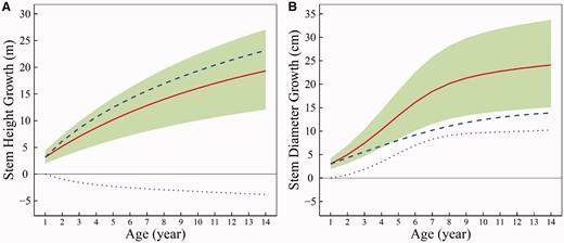
Growth trajectories of stem height (A) and diameter (B) from a full-sib family of poplar hybrids over the first 14 years of ontogeny, whose distribution and extent of genotypic variation is shown in shade. The mean curves of two growth traits, indicated by solid red lines, are well fitted by GLVDE (1). Each overall curve is the summation of independent growth curve (blue broke line) and interactive growth curve (purple dot line).
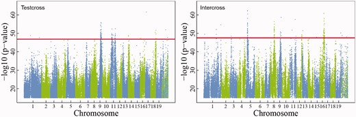
Manhattan plots of LR values over 19 chromosomes of the Populus genome, from which significant intercross and testcross QTLs are detected through permutation tests. The horizontal dash lines are the genome-wide critical threshold at the 1% significance level determined from 1000 permutation tests.
QTL mapping by game theory
The joint process of independent growth and dependent growth is further dissolved into its underlying genetic components, expressed as QTLs, using genome-wide SNP information. By estimating and testing GLVDE parameters (αH, KH, rH, βH←D, sH←D; αD, KD, rD, βD←H, sD←H) between different genotypes, we characterized how a QTL affects the relative contributions of competition and cooperation to the origin, structure and function of height–diameter allometry. Because of their different amounts of segregation information, we determined the critical thresholds for QTL detection separately for each, with Manhattan plots of test statistic values given in Figure 2. Our game theory-based mapping model identified 100 testcross SNPs and 118 intercross SNPs sporadically distributed over the genome, although some chromosomes harbor more than the others. Supplementary Table S1 gives basic information about these SNPs, including their chromosomal and physical locations, segregating types, allele types and biological function. Of these significant SNPs detected, 75 testcross QTLs (75%) and 68 intercross QTLs (58%) were found to reside within candidate genes. As a majority portion of significant SNPs are located on chromosomes 5, 8, 9, 11 and 16, we estimated their recombination fractions separately for different chromosomes (Supplementary Figure S3). Those SNPs that are highly linked on the same chromosome are likely to represent the same QTL collectively. For example, 14 highly linked SNPs on chromosome 5 reside within the region of the cystathionine beta-synthase (CBS) gene encoding a CBS domain that functions as sensor of cellular energy [48]. Eight linked SNPs on chromosome 16 that are likely to function as a single QTL are within the Neutral gene encoding neutral/alkaline non-lysosomal ceramidase [49].
MLEs of ODE parameters for different genotypes, AA and aa, at a testcross QTL by the game-theoretic QTL model from simulated growth data in an assumed full-sib family under different samples sizes and heritabilities
| True | n = 64 | n = 200 | ||||||||
|---|---|---|---|---|---|---|---|---|---|---|
| H2 = 0.05 | H2 = 0.1 | H2 = 0.05 | H2 = 0.1 | |||||||
| AA | Aa | AA | Aa | AA | Aa | AA | Aa | AA | Aa | |
| α1 | 3.713 | 12.942 | 5.281 | 6.452 | 3.421 | 11.982 | 3.810 | 13.478 | 3.660 | 13.030 |
| (3.291) | (5.963) | (0.968) | (2.629) | (2.019) | (1.981) | (0.756) | (1.954) | |||
| r1 | 41.351 | 27.729 | 26.917 | 24.505 | 50.790 | 26.730 | 41.513 | 26.525 | 41.224 | 27.350 |
| (13.092) | (15.303) | (5.872) | (3.450) | (9.652) | (4.017) | (4.552) | (1.388) | |||
| K1 | 0.323 | 0.139 | 0.499 | 0.444 | 0.286 | 0.142 | 0.335 | 0.142 | 0.319 | 0.139 |
| (1.982) | (0.505) | (0.131) | (0.346) | (0.464) | (0.082) | (0.117) | (0.203) | |||
| β1←2 | −50.882 | −55.518 | −27.560 | −31.507 | −49.647 | −57.318 | −53.085 | −55.449 | −52.087 | −54.607 |
| (11.502) | (12.809) | (8.525) | (10.165) | (10.129) | (11.439) | (8.216) | (7.492) | |||
| s1←2 | −4.110 | −2.755 | −2.229 | −1.826 | −3.939 | −2.970 | −4.197 | −2.798 | −4.150 | −2.784 |
| (1.494) | (0.950) | (0.519) | (0.809) | (1.071) | (0.623) | (0.451) | (0.414) | |||
| α2 | 1.063 | 1.772 | 1.119 | 1.701 | 1.044 | 1.543 | 1.066 | 1.708 | 1.062 | 1.789 |
| (0.723) | (0.999) | (0.348) | (0.736) | (0.371) | (0.708) | (0.309) | (0.621) | |||
| r2 | 12.411 | 16.903 | 11.50 | 15.983 | 13.564 | 19.165 | 12.528 | 17.542 | 12.453 | 16.668 |
| (4.685) | (4.117) | (1.981) | (3.673) | (2.796) | (3.292) | (1.682) | (3.170) | |||
| K2 | 4.076 | 3.488 | 3.653 | 3.527 | 3.783 | 3.748 | 4.104 | 3.522 | 4.039 | 3.533 |
| (1.324) | (1.834) | (0.495) | (0.594) | (0.742) | (0.879) | (0.373) | (0.423) | |||
| β2←1 | 0.026 | 0.077 | 0.024 | 0.073 | 0.025 | 0.081 | 0.026 | 0.079 | 0.025 | 0.079 |
| (3.458) | (1.067) | (0.177) | (0.291) | (0.082) | (0.310) | (0.072) | (0.250) | |||
| s2←1 | 2.001 | 1.469 | 1.882 | 1.324 | 1.895 | 1.344 | 2.019 | 1.435 | 1.985 | 1.445 |
| (1.449) | (0.713) | (0.496) | (0.507) | (0.371) | (0.499) | (0.296) | (0.444) | |||

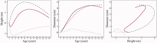
Genotypic curves of stem height and diameter growth in hybrid poplars, explained by QTL GameQ.17. The overall growth of each trait (red solid line) was contributed by independent growth (blue broke line) and dependent growth (purple dot line). Two genotypes are AG and AA.
Genetic control of height–diameter interactions
We drew genotypic overall growth curves for both height and diameter traits and further ruled out genotypic independent and dependent growth curves of each trait at each QTL detected. As an example, we chose the most significant QTL, named ‘GameQ.17’, mapped to chromosome 17. This is a testcross QTL with two genotypes AA and AG. Both genotypes at this QTL were detected to follow a similar pattern of height–diameter interaction (Figure 3). Their primary and secondary growth toward stem woody growth underlie a commensalistic symbiosis (2) by which diameter growth benefits considerably from height growth but height growth gains neither benefit nor harm from diameter growth. This can be seen from a similar form of overall growth and independent growth for stem height but greater overall growth relative to independent growth for stem diameter.
Allometry game theory can quantify the differences of two genotypes at GameQ.17 in commensalistic height–diameter relationship. Although genotypes AA and AG have a similar height growth at age 14 years, the growth curves of the former are more curvaceous than those of the latter (Figure 3). The genetic effect of this QTL on stem height growth first increases with age at an early stage, reaches a maximum value at age 6–7 years and then decreases after this peak (Figure 4A). Relative to stem height growth, this QTL has a much more pronounced effect on stem diameter growth, as shown by a noted difference in the shape of diameter growth curve between the two genotypes (Figure 3). The genetic effect on diameter overall growth increases sharply until age 10 years, suggesting that the timing of the occurrence of maximum genetic effect on stem diameter growth is delayed by about 3–4 years compared with stem height growth (Figure 4B).
The temporal pattern of pleiotropic effect on stem height (A) and diameter growth (B) and the dynamic relationship of each effect on these two growth traits (C) in hybrid poplars at GameQ.17. The genetic effects on overall growth, independent growth and dependent growth are indicated by red solid line, blue broke line and purple dot line, respectively.
It was found that GameQ.17 also exerts its genetic effects on independent and dependent growth, but in different manners (Figure 4). For stem height, this QTL has a larger genetic effect on independent growth than overall growth, although the temporal pattern of the effect is similar between these two types of growth (Figure 4A). Likewise, the effect was observed for dependent growth, but with a different direction, which reaches a valley as early as age 2 years. The two genotypes of GameQ.17 have different forms of independent and dependent growth for stem diameter (Figure 3). Its genetic effect on the independent growth of stem diameter consistently increases exponentially with age, but its effect on the dependent growth is much smaller and changes it direction during stem development (Figure 4B). The overall picture of the pleiotropic effect on stem height and diameter traits by GameQ.17 was given in Figure 4C, with a similar pattern for overall and independent growth but different from that of dependent growth.
Genetic variation in independent and dependent growth can be further dissected by interaction and scale parameters of GLVDE (1), respectively. Figure 5 shows the MLEs of each of the independent growth parameters for each genotype at GameQ.17 for stem height and diameter growth. This QTL has a greater effect on growth rate and asymptotic growth for stem height than stem diameter, although such a trait-dependent difference was not detected for the rate of convergence to asymptotic growth. Genotype AA has a greater relative growth rate (3.53) than its alternative AG (2.63) for stem height (P < 0.05), whereas such difference (0.63 versus 0.74) is not significant for stem diameter (P = 0.25). Genotype AA reaches a small asymptotic growth of stem height (46.5) than genotype AD (51.1) (P < 0.05), but these two genotypes have no difference in stem diameter asymptotic growth (10.4 versus 11.3, P = 0.33). Genotypic differences are marginally significant for the rate of convergence to asymptotic values for both stem height and diameter growth.
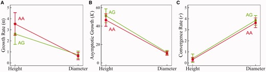
Genotypic differences in growth rate (α), asymptotic growth (K) and convergence rate (r) that determine the pattern of independent growth for stem height and diameter traits in hybrid poplars, explained by QTL GameQ.17. The 95% confidence intervals of each parameter estimate were indicated.
From GLVDE (1), we further tested how each QTL determines different aspects of dependent growth in a developmental module. By plotting the interaction and scale parameters for each genotype, we can virtualize how the two traits interact with each other and how this process is controlled by a QTL. Stem diameter growth affects negatively stem height growth at both genotypes of GameQ.17, but this effect is much more pronounced for genotype AG (–0.58) than its alternative AA (–0.05) (P < 0.01; Figure 6), suggesting that GameQ.17 has participated in the effect of diameter on height growth. Stem height growth affects positively stem diameter growth, although to a lesser extent, with genotype AA being slightly stronger than genotype AG. It was found that the strong negative effect of diameter on height growth weakens with diameter growth (because the scale parameters are negative), and this process is affected by 17, as shown by a remarkable genotype-dependent difference (Figure 6). On the other hand, the small positive effect of height on diameter growth strengthens with height growth.
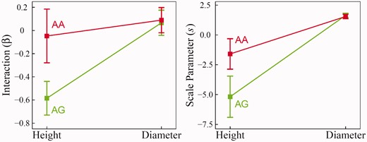
Genotypic differences in interaction (β) and scale parameter (s) that determine the pattern of dependent growth for stem height and diameter traits in hybrid poplars, explained by QTL GameQ.17. The 95% confidence intervals of each parameter estimate were indicated.
Computer simulation
To verify the utility of the game-theoretic model, we performed simulation studies by mimicking the real example of poplar trees described above. We assume two growth traits, 1 and 2, that interact developmentally through cooperation and/or competition. The ODE parameters (α1j, K1j, r1j, α2j, K2j, r2j; β1←2j, s1←2j, β2←1j, s2←1j) estimated for each genotype (j) of a testcross QTL and the SAD(1) parameters for covariance structure from the example were used as true values for simulation. We simulated a full-sib family of size n = 64 (the same as the real example) and 200 under heritabilities of H2 = 0.05 and 0.10. The size of heritability was used to adjust the magnitude of innovative variance.
We analyzed the simulated data using the new model, with results about ODE parameter estimates given in Table 1. As expected, the precision of parameter estimation increases with sample size and heritability. When heritability is small (e.g. 0.05), a small sample size (64) may give reasonable estimates although their precision cannot always be satisfied. This result suggests that the result from the above example should be interpreted with caution. However, when either heritability increases to 0.10 or sample size increases to 200, estimation precision improves dramatically. Thus, in practice, a mapping experiment should have a sample size of about 200 or phenotyping should be adequately precise to minimize noises.
Using the estimated ODE parameters, we drew growth curves for both simulated traits. It can be seen that estimated curves (including the overall, independent and interactive) are broadly in agreement with true curves under heritability of 0.05 and sample size of 64 (Figure 7). This suggests that the genotype-specific curves estimated from the above example are reasonably convincing, but given some degree of deviation from the true curves, these estimated curves should be cautious to be extrapolated. However, when heritability increases to 0.10, the curves can be estimated reasonably well, even if the sample size is still 64 (Figure 7). For those traits with low heritability, the precision of growth curve estimation can be improved by increasing sample size (Figure 8). In general, sample size of 200 is a reasonably good size for QTL mapping using our game-based model.
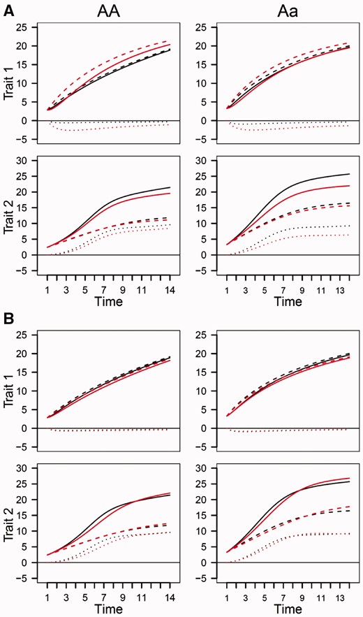
Estimated growth curves (red) of two traits for each QTL genotype, AA and Aa, from the simulated data under sample size 64 and heritabilities 0.05 (A) and 0.10 (B) by the game-theoretical QTL model, in comparison with true curves (black). Solid curves denote overall growth curves, slash curves denote independent growth curves and dot curves denote dependent growth curves.
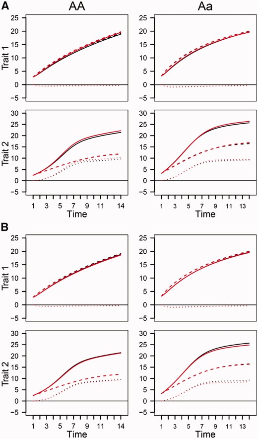
Estimated growth curves (red) of two traits for each QTL genotype, AA and Aa, from the simulated data under sample size 200 and heritabilities 0.05 (A) and 0.10 (B) by the game-theoretical QTL model, in comparison with true curves (black). Solid curves denote overall growth curves, slash curves denote independent growth curves and dot curves denote dependent growth curves.
Discussion
Stem woody production can be regarded as a developmental module composed of internally integrated elements, e.g. apical meristems leading to the lengthening of stem height and lateral meristems leading to the enlargement of stem width, which function as a whole to face environmental change [8, 50]. As such, it is reasonable to treat stem growth as an ecological system, from which to construct a new theory that quantifies the organization and function of the stem. Using game theory, we develop a conceptual framework to characterize how the underlying elements of the stem interconnect to modulate its function through competition and cooperation. We implemented GLVDE into systems QTL mapping, which can not only describe the overall growth of stem height and diameter growth, but also dissect the growth into independent and interactive parts, thus quantifying the impact of cooperation and competition on stem growth. This implementation, in conjunction with game theory, leading to allometry game theory, is particularly powerful to detect QTLs that participate in the biological coordination of competition and cooperation. By using allometry game theory to analyze stemwood growth data from a mapping experiment of poplar, the new model has successfully identified several such interaction QTLs for stem growth, such as GameQ.17 on chromosome 17 that determines commensalistic height–diameter relationship. Many of these QTLs have been observed to residue in the proximity of candidate genes with clear biological functions [48, 49].
The current model for allometry game theory focuses on analysis and modeling of the first 14 year growth which is a small portion of the long growth process of trees. Previous work on growth models shows that tree growth involves multiple phases from juvenile, adult and senescence, each of which can be fitted by a logistic curve [30]. Thus, the current model of two coupled GLVDE should be extended to include multiple phases that can characterize a complete ontogeny of tree growth. Although such extension will dramatically increase the complexity of the model and ODE parameter estimation, increasing computing efficiency through multiple tandem-driven computers can make it feasible. In our early analysis, we used traditional bivariate functional mapping to map allometry QTLs that modulate the developmental relationships of height and diameter growth using the first 24 year growth data of the same family [51]. Different sets of QTLs were identified by the traditional approach and allometry game theory model although QTL discoveries from both studies can be interpreted through gene annotations. This may be attributed to two reasons. First, the two studies used different amounts of growth data. Second, the two models may complement each other. The traditional model characterizes how one trait varies genetically with the phenotypic change of the other, whereas allometry game theory focuses on the difference of independent growth and dependent growth for a particular trait. In practice, we recommend the use of both models to dig out any possible genetic machineries underlying stem allometry.
Allometry game theory proposed in this article provides a general framework for dissecting stem allometry. By modeling allometry data from multiple environments, this theory can be extended to study how stem height growth interacts with stem diameter growth in response to environmental change. Stem growth is responsive to resource supply not only for the amount of growth but also in the allometric form of growth. Thus, by growing the same mapping population under resource-rich and resource-deficient conditions, the extended allometry game theory can characterize the discrepancy of the physiological mechanisms underlying stem height–diameter relationship in these two contrasting environments [19, 25]. This theory can further identify specific genetic loci that govern the evolutionary change of the trade-off relationship of height and diameter growth that competes for resources.
Modern genetic mapping studies have reached a point at which its permeation into various disciplines of biology has become highly essential to maximize its use [40]. Such permeation, which can be made feasible through synthesizing the common aspects of different disciplines, can shed light on fundamental biological questions, which cannot be addressed at ease. For example, developmental allometry [52] and evolutionary game model [29] are two historically disjointed concepts, but both share a common language—internal interaction. Systems mapping founded on a web of interactions within a dynamic system [40] plays a bridging role in connecting these two concepts and has been shown to be powerful for studying the genetic origin of developmental modularity through evolutionary game theory. Although the model focuses on stem allometry, its underlying principle applies to many other aspects of allometry studies, including vegetative growth versus reproductive growth, wing length versus body mass and body surface area versus body mass among others. A detailed procedure for ODE parameter and covariance-structuring parameter estimation has been implemented into a computing platform, which can be downloaded at http://ccb.bjfu.edu.cn/program.html or requested from the corresponding author.
Key Points
Stem allometry, i.e. the scaling relationship between stem height and diameter, is an important trait to ecological research and tree breeding.
The mechanistic basis for stem allometry can be investigated through modeling how primary growth interacts and coordinates with secondary growth.
We propose allometry game theory to study the ecological mechanisms of stem allometry.
The game-theoretical model provides new insight into quantifying the genetic architecture of stem allometry.
Supplementary Data
Supplementary data are available online at http://bib.oxfordjournals.org/.
Acknowledgments
We thank the three anonymous reviewers for their constructive comments, which have improved the presentation of this manuscript.
Funding
Fundamental Research Funds for the Central Universities (BLX2013011), Beijing Nova program (Z161100004916074), National Natural Science Foundation of China (31401900), grant from the State Administration of Forestry of China (201404102), the Changjiang Scholars Award and ‘One-thousand Person Plan’ Award.
Liyong Fu is working with the Center for Computational Biology at Beijing Forestry University, China. He is an associate professor in forest management in the Institute of Forest Resource Information Techniques at Chinese Academy of Forestry, Beijing, China.
Lidan Sun is a lecturer in Beijing Key Laboratory of Ornamental Plants Germplasm Innovation & Molecular Breeding, National Engineering Research Center for Floriculture, School of Landscape Architecture at Beijing Forestry University, Beijing, China.
Han Hao obtained her PhD in the Department of Statistics at The Pennsylvania State University, USA, and is currently an Assistant Professor in the Department of Mathematics at the University of North Texas, Denton, USA.
Libo Jiang is a PhD candidate in the Center for Computational Biology at Beijing Forestry University, Beijing, China.
Sheng Zhu is a lecturer in Jiangsu Key Laboratory for Poplar Germplasm Enhancement and Variety Improvement at Nanjing Forestry University, Nanjing, China.
Meixia Ye is a lecturer in the Center for Computational Biology at Beijing Forestry University, Beijing, China.
Shouzheng Tang is a professor in Forest Management in the Institute of Forest Resource Information Techniques at Chinese Academy of Forestry, Beijing, China. He is member of the Chinese Academy of Sciences.
Minren Huang is a professor emeritus in Jiangsu Key Laboratory for Poplar Germplasm Enhancement and Variety Improvement at Nanjing Forestry University, Nanjing, China.
Rongling Wu founded the Center for Computational Biology at Beijing Forestry University, Beijing, China. He is Distinguished Professor of Public Health Sciences and Statistics and Director of the Center for Statistical Genetics at The Pennsylvania State University, Hershey, USA.
References
Author notes
Liyong Fu, Lidan Sun and Han Hao authors contributed equally to this work.
