


Abstract
Statements on how the internal-to-external-dose (IED) relationship looks like are often based on qualitative toxicokinetic arguments. For example, the recently proposed kinetically derived maximum dose (KMD) states that the IED relationship must have an inflection point, due to saturation of underlying processes like metabolism or absorption. However, such statements lack a solid quantitative foundation. Therefore, we derived expressions for the IED relationship for a number of scenarios based on a generic compartmental model involving saturation. The scenarios included repeated or single dose, and saturable metabolism or saturable absorption. For some of these scenarios, an explicit expression for the IED relationship can be derived, for others only implicit expressions can be established, which need to be evaluated numerically. The results show that saturable processes will lead to an IED relationship that is nonlinear over the whole dose range, ie, it can be approximated by a linear relationship at the lower end, whereas the approximation will become gradually poorer with increasing doses. The finding that saturation does not lead to an inflection point in the IED relationship, as assumed in the KMD, implies that the KMD is not a valid approach for selecting the top dose in toxicological studies. An additional use of our results is that the derived explicit expressions of the IED relationship can be fitted to IED data, and, possibly, for extrapolation outside the observed dose range.
Toxico-(pharmaco-)kinetics is an important determinant of the final dose-response of chemicals (pharmaceuticals), which reflects the magnitude of the effect as a function of dose. When kinetic data are available, kinetic models may help in evaluating dose-response data and even be used to estimate what may happen in situations not measured (eg, human exposures). The latter is assumed to be more warranted for models with a biological basis, usually denoted as physiologically based models.
Typically, kinetic models are used to predict internal dose as a function of time. Therefore, our understanding of how internal doses may change over time is well developed, based on ample experience with toxicokinetic modeling of data for many compounds. However, the question of how internal dose may change with external dose is less often based on examination of data or on their evaluation using kinetic models. Often, the shape of the relationship between internal and external dose (briefly, the IED relationship) is based on assumptions. For example, it is usually assumed that at low doses saturation cannot play a role, and hence kinetics will be first order, resulting in the internal dose being proportional to the external dose, also denoted as linear. Only at higher doses, where saturation does play a role, linear kinetics will turn into nonlinear. In kinetic modeling, this idea is often used as a condition for simplifying the model: As long as doses are low enough the model can be based on first-order kinetics, which makes the model simpler (ie, fewer parameters).
The idea of an IED relationship that changes from linear to nonlinear due to saturation of underlying processes has recently found a specific application: The kinetically derived maximum dose (KMD) to be used as the top dose in toxicity studies. The assumption is that doses where saturation occurs are not relevant for humans, as human exposure is typically too low for reaching saturation, and hence it would not be needed to test these doses. Authors discussing the KMD (eg, Barton et al., 2006; Creton et al., 2012; Saghir et al., 2013; Sewell et al., 2017; Terry et al., 2016) further assume that the IED relationship has an “inflection” point, ie, the dose where the internal dose stops to increase in proportion with external dose, due to saturation. The existence of an inflection point, as in Figure 1, is based on qualitative thinking, whereas the underlying processes are quantitative. In particular, the inflection point is imagined to occur at a dose where saturation occurs. However, saturation of enzymes will be some quantitative value within the range of 0% and 100%, which depends on dose, whereas 0% does not exist (there will always be ligand molecules that bind to the enzyme), nor does 100% (there will always be enzyme molecules that just released their ligands). Therefore, the alleged inflection point in the IED relationship is based on a qualitative (binary) simplification of the quantitative phenomenon saturation. Predicting by mental imagination how interacting dynamic processes work out is virtually impossible: The human mind falls short here. A reliable understanding of how internal dose may change with external dose can only be achieved by using a well-defined kinetic model, which reflects the main dynamic processes of interest or relevance. For the purpose of examining the shape of the IED relationship, the model does not need to be a full physiologically-based model, as the interest is not to get a reliable extrapolated internal dose for a single specific compound. All we want is a better understanding of the shape of the IED relationship, in a general sense, and for some of the main scenarios occurring in toxicity testing. Therefore, we will take the most simple kinetic model possible as the starting point; the simpler the model, the more likely it is that an explicit expression for the IED relationship can be found. An explicit expression has the advantage of giving generic insight in the shape of the relationship, and further, that it can be fitted to a given dataset (as illustrated below).
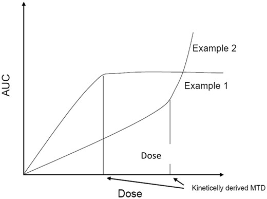
The hypothetical relationship between internal dose (eg, AUC) and external dose which, according to some authors, has an inflection point (indicated by the vertical lines) due to saturation, where the lower linear part of the relationship changes into nonlinear (ie, internal dose is no longer proportional to external dose). One curve (example 1) is assumed to follow from saturation of absorption and the other (example 2) from saturation of metabolism of the parent compound. Figure adapted from ECHA (2017).
DEFINITION OF MODELS
We defined 2 models for evaluating 4 scenarios: a model with saturable metabolism (Figure 2) and a model with saturable absorption (Figure 3). The model with saturable metabolism was used for 3 different dosing scenarios: long-term (constant) dosing (scenario 1), single intravenous dose (scenario 2), and single oral or intraperitoneal dose (scenario 3). The other model was used for a single oral dose (scenario 4). Because our aim was to derive explicit expressions for the IED relationships, we did not consider more complicated scenarios: Already some of these simple scenarios turned out to result in implicit expressions that could not be further solved.
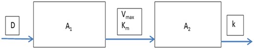
The basic compartmental model, with A1 reflecting the amount of the parent, and A2 the amount of one of its metabolites.
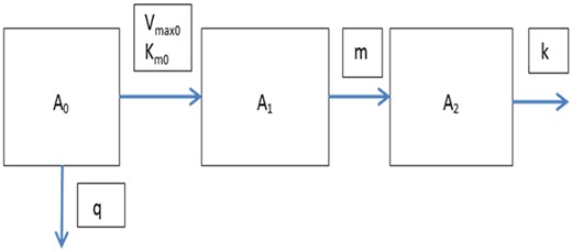
The basic model extended with a gut compartment, with A0 reflecting the amount of the parent in the gut. Absorption is assumed to be subject to saturation described by Vmax0 and Km0. Further, excretion from the gut is assumed to be first order with rate parameter q.
The model with saturable metabolism is illustrated in Figure 2. It consists of a compartment reflecting the amount of the parent compound (A1) and a compartment reflecting the amount of its metabolite (A2). The 2 compartments may be envisaged as a specific organ (eg, the liver), or as the whole body. As long as the concentration (C) in the whole body (body burden) is proportional to that in each individual organ, this makes no difference for the shape of the IED relationship. The volume of each of the 2 compartments (physically the same) is denoted as V, and assumed to be constant in time (no growth). The metabolism of the parent (with amount A1) into its metabolite (with amount A2) is governed by parameters Km and Vmax, the typical Michaelis-Menten constants for saturable metabolism. The metabolite is assumed to be excreted with a constant (first-order) rate k. In principle, excretion or further metabolism may be saturable as well, but it is often assumed that phase II enzymes are available in excess and that the first metabolic step is rate limiting.
The model with saturable saturation is illustrated in Figure 3. It is used for scenario 4, where it is assumed that a single dose is absorbed by a saturable mechanism in the gut. To mimic this scenario, an additional compartment is included in the model, reflecting the gut. The absorption occurs at a rate which is restricted by the level of saturation of the absorption mechanism. We describe the absorption by a Michaelis-Menten relationship, with constants Vmax0 and Km0. In this case, it will be assumed that the metabolism of the parent can be approximated by first-order metabolism with a single rate constant m. This should be a reasonable assumption if absorption is the rate-limiting process. In the opposite case, where metabolism is rate limiting, absorption can probably be approximated by a first-order process, which amounts to the third scenario already discussed.
RESULTING IED RELATIONSHIPS
This section discusses the resulting IED relationships for each of the 4 scenarios consecutively. Table 1 summarizes the resulting expressions. The underlying mathematical derivations are shown in the Appendices 1–4.
IED Relationships for the 4 Scenarios
| Saturable Process | Parent Compound | Metabolite | |
|---|---|---|---|
| Scenario 1: Long-term constant dose | Metabolism (elimination) | ||
| Scenario 2: Single IV dose | Metabolism (elimination) | ||
| Scenario 3: Single oral or IP dose | Metabolism (elimination) | Cannot be proven, but probably similar to scenario 2 | |
| Scenario 4a: Single oral dose | Absorption |
The relationships given here are the first-order approximations. As Figure 6 shows, with higher dose this approximation will get worse.
Scenario 1: Repeated Dose With Saturable Metabolism
We first consider the situation of repeated dose, by assuming a constant dose rate over time (denoted by D). A constant dose rate could reflect continuous intravenous administration, or the inhalation of a constant concentration over a longer period of time. Under these conditions, the internal dose will reach a steady state at some point in time. In oral repeated dose studies, the dose is usually administered in one (eg, gavage) or a few time periods (eg, meals) on each day, so that the dose rate is, strictly speaking, not really constant (ie, at smaller time intervals). However, as long as half-life is relatively long, the internal dose will reach a (pseudo) steady state, ie, with levels fluctuating around the steady state. Therefore, we will approximate the situation with one or various dose events per day as a constant dose rate, if the chemical has a relatively long half-life (and similar dose amounts per day). For chemicals with a relatively short half-life, the internal concentration just before the next dose event will be close to 0, and the repeated dose scenario may be treated as a single dose scenario (see scenario 2 or 3 below). In scenario 1, we consider the steady-state internal concentration as the internal “dose” in the IED relationship. The AUC is less useful in this case, as it will keep increasing when exposure continues. Further, we define D as a constant (external) dose rate, expressed as amount per time unit.
As C1 cannot be negative, it follows that Vmax > D/V, which equals the steady-state condition (see Appendix 1). Figure 4 (upper panel) illustrates the relationship for C1 for specific values of the parameters. Here, the parameter values as mentioned in the figure legend, as well as the scales of the plot, have no dimension, as they are not directly relevant for the shape of the relationship. The lower panel of Figure 4 shows the dose-adjusted internal dose, ie, the internal dose divided by the external dose D, as a function of dose. It shows that the dose-adjusted internal dose increases as soon as external dose is larger than 0. This can also be seen directly from expression (1): dividing by D results in an increasing function without a horizontal plateau. This shows that there is no horizontal plateau which would be needed to have linearity at low doses.
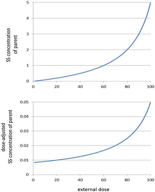
Internal-to-external-dose (IED) relationships for scenario 1. Upper panel: steady-state (SS) concentration of the parent according to theoretical relationship (1), for Km = 1, Vmax = 0.12, and V = 1000 (arbitrary units). Other values for these parameters result in other relationships, but with similar shapes. In this case, steady state will be reached for doses lower than V × Vmax = 120. Lower panel: same relationship after dose adjustment (= steady state divided by external dose). Even at very low doses, this relationship is increasing.
Scenario 2: Single Intravenous Dose
When a single dose is administered intravenously, the dose can be considered as being systemically available instantaneously. This scenario can be modeled by changing the initial conditions for the model equations used in the previous case (see Appendix 1). For single dose scenarios, the AUC is a relevant measure of internal dose, defined as the area under the curve of the relationship between internal concentration and time. For mechanisms of action where the peak concentration is considered a more relevant measure of internal dose, it may be noted that the AUC and the peak concentration are strongly correlated, and the shape of the IED relationship will not be substantially different.
Figure 5 shows the shapes of the IED relationship according to expression (3), as well as that of the dose-adjusted IED relationship. From expression (3), it follows directly that the dose-adjusted AUC is a linearly increasing relationship with dose D (also see Figure 5, lower panel).
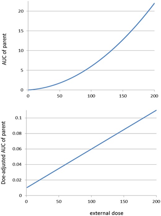
IED relationships for scenario 2. Upper panel: AUC of the parent according to theoretical relationship (3), for Km = 0.01, Vmax = 1, and V = 1000 (arbitrary units). Other values for these parameters result in similar shapes. Lower panel: same relationship after dose adjustment (= AUC divided by external dose D). The relationship is increasing as soon as the external dose D > 0. The dose-adjusted AUC value at dose 0 is Km/Vmax, derived as the limit of expression (3) divided by D for D -> 0.
Scenario 3: Single Oral or Intraperitoneal Dose
When a single dose D is administered orally or intraperitoneally (IP), there will be a time delay before the complete dose becomes systemically available. This is usually modeled by multiplying the dose by an exponential function which decreases over time to 0 (asymptotically).
Scenario 4: Single Oral Dose With Saturable Absorption
As Appendix 4 shows, this scenario does not allow for an explicit solution for the AUC of the parent, nor of the metabolite. Therefore, the IED relationship can only be calculated numerically. Figure 6 shows a numerically calculated IED relationship, which is nonlinear for both the parent and the metabolite. When other parameter values were used to calculate the IED relationship its shape did not fundamentally alter, ie, it was always nonlinear without infection point. In Table 1, approximate expressions are given for the IED relationships of the parent and the metabolite.
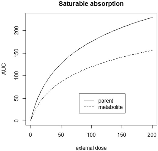
IED relationship for scenario 4. Note that the shape is nonlinear over the whole dose range. Parameter values used: Km0 = 0.1, Vmax0 = 1, V = 50, q = 0.5, m = 0.1, and k = 0.1 (see Figure 3, or Appendix 4, for notation).
APPLICATION TO A REAL DATASET
Saghir et al. (2013) and Saghir and Dorato (2016) published an extraordinarily large dataset of AUCs established in an extended one-generation reproductive toxicity study with the compound 2,4 Dichlorophenoxyacetic Acid (2,4-D). The animals were exposed to repeated dietary doses during around 3 months, starting 2 weeks before mating. AUCs were estimated at the end of the exposure period based on 3 blood samples (on the same day). The authors plotted the estimated AUC values against external dose (as reproduced in Figure 7, left panel) and visually drew a straight line at the lower end, which they considered to represent the linear relationship between AUC and external dose at lower doses. Next, they claimed an inflection point at around 50 mg/kg/day. However, interpreting a visual pattern when doses and AUCs are plotted on the original scales is misleading. For example, in such plots, the distance between an AUC of 1 and 2 units is considered equivalent to the distance between 7001 and 7002 units. Clearly, this is not reasonable. For a biologically reasonable interpretation, a double-log-plot is more appropriate, as on log-scale ratios between numbers are considered equivalent (see the Discussion section for a more extensive discussion on linearity and plotting data). A first point to note is that the scatter between the points in the right plot of Figure 7 (double-log-scale) does not increase with higher AUCs, as in the left plot of Figure 7 (original dose-scale). This means that the scatter, expressed as a coefficient of variation, is homogenous over the whole dose range. More important, the right panel of Figure 7 shows that there is in reality no point of inflection. The point of inflection that seems to exist in the left plot is just a visual artifact resulting from the apparent increase in the scatter when the data are plotted on the original dose-scales. Because a difference between 1 and 2 dose units is biologically not the same as between 7001 and 7002 dose units, the original dose-scale is inappropriate for visual interpretation. On log-scale, a difference between 1 and 2 dose units is considered equivalent with that between 1000 and 2000 dose units.
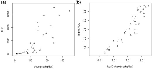
Plot of observed AUCs of 2,4-D against external dose, as (numerically) reported by Saghir and Dorato (2016). In the left panel, both AUCs and external doses are plotted on the original scales. Saghir and Dorato (2016) derived a kinetically derived maximum dose (KMD) from a similar plot by drawing a straight line through the points at the lower end, claiming an inflection point at around 50 mg/kg/day. In the right panel, both AUCs and external dose are plotted on log-scales, showing that in reality there is no point of inflection. The left plot is misleading (see main text and Heringa et al., forthcoming).
The chemical 2,4-D is rapidly eliminated (T1/2 = 2–3 h) without or hardly being metabolized (Hayes and Wayland, 1982; Milby, 1980). Furthermore, the elimination of 2,4-D in the kidney is saturable (Saghir et al., 2013). Although not evident at first sight, scenario 2 (single instantaneous dose, with saturable metabolism), resulting in relationship (3), would be (approximately) appropriate for these data, for the following reasons. Although Saghir et al. applied repeated dose (for various weeks), the scenario of a single dose seems to apply in this case, as the internal dose will start at virtually 0 on every new day of exposure, due to the very short half-life. Further, the scenario of a compound not being metabolized but excreted via a saturable process is quantitatively similar to the scenario of being metabolized by a saturable enzyme. And, finally, although the dose was administered via the food, we use the scenario of intravenous administration as an approximation, which has the advantage of resulting in an explicit expression for the IED relationship. As already noted, the retardation in scenario 3 as compared with scenario 2 will hardly have an impact on the AUC. Therefore, we fitted expression (3) to the observed data, using the PROAST software (https://www.rivm.nl/en/proast; last accessed June 15, 2020), where expression (3) is implemented as model 55.
Saghir et al. used various experimental groups (2 generations, 2 genders, various ages), for which the parameters Km, Vmax, and V in expression (3) might be different. PROAST allows to fit the model to all experimental groups combined, while assuming that one of the parameters depends on the experimental group. We found that the best fit was obtained by letting PROAST estimate different subgroup-specific values for parameter V, representing the volume of the organ that metabolizes or eliminates the compound (the estimated values for V appeared to be roughly in line with age and sex of the experimental groups). The 2 other parameters, Vmax and Km, were assumed to be the same for all groups. These 2 values could not be separately estimated (identified), ie, one of them could be fixed at any arbitrary value before fitting the model, without resulting in a poorer fit. As Figure 8 shows, the fit was remarkably accurate. The fluctuations of some of the data around the fitted curves can be explained by the expectation that the observed AUCs are subject to considerable estimation errors, as they were based on only a limited number of measured internal concentrations in time.
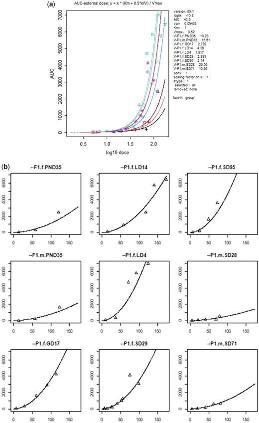
Expression (3) fitted to AUC data (Saghir et al., 2013) as a function of dose, using experimental group as a covariate. In the left plot, the fit is shown for all 9 experimental groups in one plot. In the right plot, they are shown separately. Note that in the left plot, the data and the model are plotted against log-dose, in the right plot against dose (but they both show the same data and fitted curves; the different shapes are just a matter of scales used). Parameter Km was fixed at the arbitrary value 1 in fitting the model, as it could not be estimated independently from Vmax.
DISCUSSION
One of the reasons of examining the IED relationship with a toxicokinetic model was to answer the question whether or not the alleged existence of an inflection point, at the point where saturation occurs, stands scrutiny. We doubted that assumption, as saturation is not an event, which switches “on” at a given dose, but a quantitative phenomenon, with a value that can be anything between 0% and 100%. The results from our kinetic models unambiguously show that an inflection point, as a result of saturation, does not exist. Clearly, the conclusion on the nonexistence of an inflection point has consequences for the recently proposed method of the KMD (eg, Creton et al., 2012; Domoradzki and Boobis, 2018; Saghir et al., 2013; Sewell et al., 2017), which relies on the existence of an inflection point. Our conclusion undermines the very basis of the KMD approach, as it follows that this approach tries to estimate a point that does not exist. Apart from the nonexistence of an inflection point, there are various other reasons why the KMD approach is not recommendable, as discussed in a critical review by Heringa et al. (forthcoming).
One of the arguments behind the KMD method is that it is not useful to test doses where the internal dose no longer changes, as in IED relationships that level off (see example 1 of Figure 1). One of the alleged mechanisms underlying a leveling-off IED relationship is saturated absorption. However, as Figure 6 shows, in this scenario, the internal dose does keep increasing with higher doses, be it at gradually decreasing speed. An IED relationship that levels off was also claimed to occur for a metabolite with saturated metabolism of the parent. However, as expressions (2) and (4) show, the IED relationship of the metabolite was found to be linear, as long as saturation of excretion (or further metabolization) of the metabolite itself can be ignored. If such cannot be ignored, the IED relationship of the metabolite will become nonlinear, obviously not with an inflection point, but with a shape similar to that shown in Figures 4 and 5 (upper panels), ie, the curve increases even more rapidly at higher doses. In our analyses, we show that the IED relationship does not level off (to an asymptote) in any of the scenarios. Therefore, the associated argument that there would be no need to test at doses higher than the KMD—where the internal dose no longer increases—cannot be maintained.
Our findings illustrate that it is difficult to qualitatively describe toxicokinetic processes or even qualitatively predict a generic thing like the shape of the IED relationship, based on mental imagination alone. Although “mental models” can easily be misleading in general, this particularly holds for kinetics: The human mind is not fit for imagining how dynamic processes like kinetics work out without the aid of a mathematical model. Next to the intuitive illusion of an inflection point, another example that intuition can be easily misleading is given by the linear relationship of the metabolite in expressions (2), (4), and (5). How can this relationship be linear when the IED relationship of the parent slows down? The answer is that intuitive thinking tends to overlook relevant factors, in this case the factor of time. In scenario 1, the explanation is that saturation will have an impact on the time at which steady state is reached, but not on the level of the steady state itself. In scenario 2, the shape of the internal dose profile will change (become more flat), but the area under the curve remains the same.
Our analysis of the data from Saghir et al. (2013) illustrated that the definition of linearity and the visual interpretation of plotted data may need some further discussion. Linearity is often defined by visual inspection of the data: When the plotted data follow a straight line the relationship is called linear. However, the visual shape of a relationship strongly depends on the scales that are used. For example, internal doses that follow a straight line when plotted against external dose on the original dose-scales will show a sublinear pattern when plotted against log-dose. Or, nonlinear relationships on the original scales may turn into (visually) linear on double-log-scale. On other scales, the relationship will again show other visual shapes (eg, Slob, 2007), even though the relationship itself does not change. Therefore, the visual shape of a relationship can be easily misleading (Slob and Setzer, 2014). A more sound definition of a linear IED relationship is: the internal dose increases in proportion to the external dose. As the internal dose will be 0 when the external dose is 0, this definition results in a straight line when plotted on the original dose-scales. So, in the case of IED relationships, a visual straight line on the original dose-scales coincides with the definition of linearity in terms of proportionality (note that this property is lost as soon as a straight line does not go through the origin). However, equating a visual straight line (through the origin) with proportionality only holds for a theoretical relationship derived from a mathematical model (as in Figures 4–6). As soon as linearity is evaluated based on experimental data, a complication arises that needs to be taken into account: Experimental data show scatter, and usually in a way that is poorly represented by the original dose-scales. For example, on the original scale scatter in the range between 1 and 2 mg/kg is, visually, the same as scatter between 1001 and 1002 mg/kg. However, this does not reflect biological interpretation where the former scatter will be regarded as much larger than the latter scatter. Related to this notion, biological data tend to be lognormally distributed rather than normally, whereas SDs tend to proportionally increase with the mean (see eg, Slob, 2017, Supplementary Material, for extensive experimental evidence). The proportional increase of the SD with the mean implies that data will show more scatter with increasing values, when plotted on the original scale. However, in terms of coefficients of variation, the scatter does not increase with increasing values. Or, when plotted on log-scale, the scatter does not visually increase with increasing values. For these reasons, visual interpretation of data on the original scales can be misleading, and data should always be plotted on log-scales before drawing conclusions based on visual patterns. More appropriately, the data should be analyzed statistically, so that the role of sampling error is taken into account based on a plausible assumption on scatter. For example, one may fit the power model (y = axb), assuming the data to be lognormally distributed, and then evaluate if the confidence interval of parameter b includes the value of 1. Note that parameter b is the slope of the line on double-log-scale or the power parameter on double-original scale. When the slope of the line on double-log-scale deviates from unity, the relationship on the original scales will be nonlinear (nonproportional).
Our analyses show that the IED relationship is nonlinear over the whole dose range. This is in contrast to the way the impact of saturation on the IED relationship is often expressed by experts in toxicokinetic modeling: as being linear at low doses and changing into nonlinear at higher doses. A linear IED relationship would imply that the slope does not change with external dose, and hence, that the dose-adjusted internal dose (reflecting the slope of the IED relationship) would not change at lower doses. However, the dose-adjusted internal dose increases already at low dose (see lower panels in Figures 3 and 4). This seems to contradict the intuitive notion that at low doses saturation can hardly have any impact, and hence the IED relationship should be linear at the lower end of the curve. The point here is that a plot where the x-axis represents dose in the original units is easily misleading, as just discussed. For instance, the lower panel of Figure 5 suggests that a dose of 1 dose units is close to 0. However, a dose of 1 dose units (eg, mg/kg) is at least 20 orders of magnitude away from doses consisting of a few molecules, and in that huge range the change in slope of the IED relationship is indeed very small. Thus, it can be seen that saturation does have a negligible impact at low doses and the IED relationship is indeed close to linear in that dose range. However, just like saturation is not a yes/no phenomenon, a transition between linear and nonlinear does not exist. In reality, the IED is approximately linear (proportional) at low doses, and the approximation to linearity (proportionality) becomes worse with increasing doses. Hence, a better way of phrasing the impact of saturation is: The IED relationship is approximately linear at low doses, and the approximation will get gradually worse when larger dose ranges are considered (and vice versa).
DECLARATION OF CONFLICTING INTERESTS
The authors declared no potential conflicts of interest with respect to the research, authorship, and/or publication of this article.
FUNDING
Dutch Ministry of Agriculture, Nature and Food Quality.
ACKNOWLEDGMENTS
We are grateful to Peter Bos and Bas Bokkers for their valuable comments.
APPENDIX 1: REPEATED DOSE WITH SATURABLE METABOLISM
So, the necessary condition for the existence of an equilibrium is a > b, or in original parameter terms:
APPENDIX 2: INSTANTANEOUS (IV) DOSE
Explicit Derivation of Y(t)
APPENDIX 3: IP OR ORAL DOSE
So, , and the AUC of the metabolite is .
This formula equals the one that can be derived based on the differential equation for x(t) in case of the instantaneous dose (see Appendix 2). There we found, that X(∞) was nonlinearly dependent on b and thus on dose, so we expect the same dependency in this case.
APPENDIX 4: SINGLE DOSE WITH SATURABLE ABSORPTION
The AUC’s are calculated as , and .
REFERENCES
ECHA. (
Heringa, M., Cnubben, N. H. P., Slob, W., Pronk, M. E. J., Muller, A., Woutersen, M., and Hakkert, B. C. Use of the kinetically-derived maximum dose concept in selection of top doses for toxicity studies hampers proper hazard assessment and risk management. Regul. Toxicol. Pharmacol. (forthcoming).

Comments