


Abstract
A protein superfamily contains distantly related proteins that have acquired diverse biological functions through a long evolutionary history. Phylogenetic analysis of the early evolution of protein superfamilies is a key challenge because existing phylogenetic methods show poor performance when protein sequences are too diverged to construct an informative multiple sequence alignment (MSA). Here, we propose the Graph Splitting (GS) method, which rapidly reconstructs a protein superfamily-scale phylogenetic tree using a graph-based approach. Evolutionary simulation showed that the GS method can accurately reconstruct phylogenetic trees and be robust to major problems in phylogenetic estimation, such as biased taxon sampling, heterogeneous evolutionary rates, and long-branch attraction when sequences are substantially diverge. Its application to an empirical data set of the triosephosphate isomerase (TIM)-barrel superfamily suggests rapid evolution of protein-mediated pyrimidine biosynthesis, likely taking place after the RNA world. Furthermore, the GS method can also substantially improve performance of widely used MSA methods by providing accurate guide trees.
One of the grand challenges in evolutionary biology is the phylogenetic analysis of a protein superfamily that contains remote homologs, proteins that share a very distant evolutionary origin (Rojas et al. 2012). The early evolution of protein superfamilies is of particular interest because it would tell us how the building blocks of life were established or how living things and the earth coevolved in their early histories (Gaucher et al. 2010). Moreover, the recent massive accumulation of sequence data is increasing the need for reconstructing large phylogenetic trees that include remote homologs (Warnow 2013). Whereas protein superfamilies are usually identified based on structural similarity, a sequence-based approach is needed for their phylogenetic analysis because sequence data can be obtained and analyzed in a highly systematic manner (Matsuda et al. 2003). However, the existing widely used molecular phylogenetic methods (e.g., Neighbor-Joining (NJ) (Saitou and Nei 1987), maximum likelihood (ML) (Felsenstein 1981), Maximum Parsimony (MP) (Camin and Sokal 1965), and Bayesian Inference (BI) methods (Yang and Rannala 1997)) show poor performance when applied to protein superfamily-scale data sets (Chan and Ragan 2013).
The most fundamental problem in the phylogenetic analysis of a protein superfamily is that remote homologs substantially increase the difficulty of constructing an informative multiple sequence alignment (MSA) (Ogden and Rosenberg 2006). Accumulating evidence suggests that the quality of an MSA critically affects the performance of the existing methods (Tan et al. 2015). Even classical procedures in phylogenetic analysis, such as constructing and filtering of MSA, are now being critically re-evaluated (Tan et al. 2015). To avoid the problem of the dependence on informative MSA, it has been proposed to use all-to-all pairwise sequence alignment (PSA) for calculating distance matrices and reconstructing phylogenetic trees using the NJ method (Thorne and Kishino 1992). Indeed, the pioneering studies showed that such PSA-based NJ methods (e.g., PhyPA) can outperform the ML and BI methods when data sets contain remote homologs (Xia 2016), suggesting that phylogenetic tree reconstruction based on distance matrices (or sequence similarity graphs [SSGs]) created by all-to-all PSA is promising for estimating protein superfamily-scale trees. It may also be notable that such a graph- or network-based approach has been successfully applied to analyze complex evolutionary histories, such as those of fusion proteins, haplotype genomes, and viruses (Bansal and Bafna 2008; Zhang et al. 2011; Jachiet et al. 2013; Corel et al. 2016). As a graph- or network-based tree reconstruction method, the Buneman tree method was previously proposed (Buneman 1971); however, this method requires large computational cost (Bryant and Moulton 1999) and cannot reconstruct superfamily-scale trees accurately (Besenbacher et al. 2005).
Here, we propose the Graph Splitting (GS) method, which rapidly reconstructs a protein superfamily-scale phylogenetic tree that contains remote homologs. Evolutionary simulation showed that the GS method can accurately reconstruct phylogenetic trees and be robust to major problems in phylogenetic estimation when sequences are substantially diverged. In addition, to statistically evaluate branch reliabilities like the bootstrap values and posterior probabilities do, the Edge Perturbation (EP) values were introduced for the GS method. An application of the GS method to an empirical data set of the triosephosphate isomerase (TIM)-barrel superfamily suggests rapid evolution of protein-mediated pyrimidine biosynthesis, likely taking place after the RNA world. Furthermore, it was also shown that the GS method can substantially improve performance of widely used MSA methods by providing accurate guide trees.
Materials and Methods
Overview
The overview of the GS method is shown in the top panel of Figure 1a. In brief, given a set of protein sequences, the GS method first calculates symmetrical relative sequence similarities by performing all-to-all PSA using MMSeqs2 (Steinegger and Söding 2017) and obtains a weighted and undirected SSG, whose nodes and edges represent the proteins and detected similarities, respectively. Then, the node-set in SSG is recursively split in a top-down manner by the spectral clustering algorithm (Paccanaro et al. 2006) until a tree (dendrogram) is obtained (Supplementary Fig. S1 and Text S1 available on Dryad at http://dx.doi.org/10.5061/dryad.ps0qf4r.). The spectral clustering method was adopted because it shows better performance than other methods, such as component analysis, hierarchical clustering, and the Markov cluster algorithm for protein family classification (Paccanaro et al. 2006). To make the method scalable to huge data sets, we devised an approximate and fast algorithm for minimizing the normalized cut (|$N_{\rm cut})$| values (Shi and Malik 2000), which are used in the clustering algorithm.
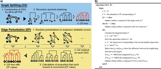
GS and EP methods. a) Schematic diagrams of the methods. The GS method builds an SSG in which nodes and edges represent proteins and sequence similarities, respectively. The SSG is then recursively split by spectral clustering, and its clustering hierarchy produces a phylogenetic tree (dendrogram). The EP method evaluates the reliability of each phylogenetic branch by performing three steps. First, the sequence similarity scores of an SSG are randomly perturbed to produce a large number of SSGs. Second, the GS method is run on each SSG to reconstruct a phylogenetic tree. Third, a recovery rate is obtained for each branch in the original tree. b) The pseudocode of the GS method.
Aside from accurately reconstructing trees, any practical phylogenetic method needs to be able to provide reliability measurements on the estimated branches, such as the bootstrap values and posterior probabilities that are used in existing methods (Felsenstein 1985). These two measures cannot be easily obtained for a method that does not rely on MSA because their calculations require an informative MSA whose columns are independent. To overcome this obstacle, we developed the EP method for statistically evaluating branch reliability (Fig. 1a, bottom). Based on the fact that sequence similarity scores follow the extreme value distribution (Bastien and Maréchal 2008), the EP method repeatedly makes random perturbations to the scores. Subsequently, the GS method is run using the perturbed SSGs, and the proportion of times that each phylogenetic branch is recovered is calculated (this is called the EP value).
GS Method
Based on the theoretical background above, the GS method recursively splits the input node-set |$V $|until a tree (or dendrogram) is obtained by the method that is represented as pseudocode (Fig. 1b). The GS method is implemented in C++ (sources and binary packages are freely available at https://github.com/MotomuMatsui).
EP Method
The EP method provides reliability measures of branches estimated by the GS method and is analogous to the bootstrap values and posterior probabilities used in existing methods. The brief procedure of EP method is that 1) a Gumbel distribution is fitted to the observed distribution of sequence similarity scores, 2) randomized sequence similarity scores are sampled from the distribution, and 3) trees are repetitively reconstructed by the randomized sequence similarity scores using the GS method.
Reconstruct a tree |$T_{0}$| by applying the GS method to |$G$|.
Induce random perturbations to |$W$| according to the extreme value distribution with parameters location=|$w_{ij} $|, scale=|$w_{ij} \left( {1-w_{ij} } \right)/3.5$|, and shape=|$e^{-3w_{ij} }-1$|.
Reconstruct a tree |$T_{EP}$| using the GS method.
Repeat steps 2–3 |$N$| times.
Calculate the recovery rate of each branch of |$T$| in |$T_{EP}s$|.
The EP method is implemented in C++.
Evolutionary Simulation
We generated 2,400 trees that had 20 external nodes. The tree shapes were randomly determined by the backward Yule process with a constant birth rate (one per unit time) using Bio::Tree::RandomFactory in BioPerl 1.6.924 (Stajich et al. 2002). Under this model, the lengths of the edges follow |$1-\ln \left( {\mbox{rand}\left( 1 \right)\times \left( {e-1} \right)+1} \right)$| substitution/site, where |$\mbox{rand}\left( 1 \right)$| represents a uniform random variable between 0 and 1. For each 400 trees, we applied different scaling factors (0.1, 0.2, 0.5, 1.0, 1.5, and 2.0) to shrink or expand the whole trees, and we prepared trees of various sizes. For each tree, the molecular evolution of a 1000 amino-acid protein sequence was simulated using the WAG+|$\Gamma $| substitution model (Whelan and Goldman 2001) with four different indel frequencies that followed the Zipfian (power-law) model (Fletcher and Yang 2009) using INDELible v1.03 (Fletcher and Yang 2009). The scaling parameter of the power-law distribution was set to the default value (1.7). The indel frequencies were set to 0.0, 0.02, 0.05, or 0.1 relative to the substitution rate (note that 600 simulations were performed for each indel frequency). We also performed simulations for different tree sizes (50, 100, and 200 external nodes) and different protein lengths (500 and 2,000 amino acids) with the same settings. For comparison with PhyPA (Xia 2016), we performed simulations with “AABlosumSym,” “AABlosumSymHalf,” “AABlosumAsym,” and “AABlosumAsymHalf” models using INDELible. Here, the comparison was conducted separately because PhyPA is a GUI tool, but under the same conditions of the PhyPA paper. Briefly, evolutionary simulation of 24 amino-acid sequences was conducted under conditions that tree topology and each interior branch length were symmetrical and 0.6 substitutions/site, symmetrical and 0.3 substitutions/site, asymmetrical and 0.3 substitutions/site, and asymmetrical and 0.15 substitutions/site, respectively.
To evaluate the performance of each phylogenetic method in the face of typical problems (biased taxon sampling, heterogeneous evolutionary rates, and long-branch attraction), additional simulations were performed. Because the simulation settings were almost unchanged from the original simulation, only the differences are described here. For simulation under biased taxon sampling, we generated 32-taxon trees that had eight different tree topologies, where topologies 1 and 7 were the most biased among the first seven and topology 8 was a complete pectinate tree (Fig. 4a, b). For each topology, four trees whose branch lengths were 0.1, 0.2, 0.5, or 1.0 substitution/site were prepared. Four indel frequencies were tested as in the original simulation. For each condition, 100 independent evolutionary simulations were performed (i.e., |$8 \times 4 \times 4 \times 100 = 12, 800$| simulations in total). For simulation under heterogeneous evolutionary rates, we used 32-taxon trees whose branch lengths were sampled from a normal distribution (using the rnorm function in R 3.4.3 (R Core Team 2015)) (Fig. 4d, e). For the branch lengths, the mean was set 0.1, 0.2, 0.5, or 1.0, and the standard deviation was set to 0.0, 0.1, 0.2, 0.5, or 1.0. Four indel frequencies were tested as in the original simulation. If negative branch lengths were obtained, they were set to 0. For each condition, 100 independent evolutionary simulations were performed (i.e., |$4 \times 5 \times 4 \times 100 = 8,000$| simulations in total). For simulation under long-branch attraction, we prepared 32-taxon trees that had two long branches (Fig. 4g, h). The lengths of the short branches were set to 0.1, 0.2, or 0.5, and the ratio between the lengths of the long and short branches was set to 1, 1.5, 2.0, 2.5, or 3.0. Four indel frequencies were tested as in the original simulation. For each condition, 100 independent evolutionary simulations were performed (i.e., |$3 \times 5 \times 4 \times 100 = 6,000$| simulations in total).
Phylogenetic Tree Reconstruction
MSA of the amino-acid sequences was conducted using MAFFT (mafft-linsi) v7.273 (Katoh and Standley 2013) with the default options. Distance matrices used in the MSA-with-complete-gap-deletion and the MSA-with-pairwise-gap-deletion approaches of the NJ method were computed using the phangorn 2.4.0 package (Schliep 2011) on R environment with the WAG+|$\Gamma $| substitution model and dist.ml function with parameter exclude=“all” and “pairwise,” respectively. Distance matrices used in the pairwise-gap-alignment approach of the NJ method were calculated based on the sequence similarity score. Phylogenetic reconstruction was conducted using the same package. Bootstrap values were computed using the bootstrap.phyDat function of the same package (bs = 100). For comparison, the NJ+PhyD* (Criscuolo and Gascuel 2008), BioNJ (Gascuel 1997), and BioNJ+PhyD* methods were also tested but showed little difference. In addition, PhyPA in DAMBE v7.0.12 (Xia 2018) was run to reconstruct PSA-based phylogenetic trees with options of gap open = 20, gap extension = 2, substitution matrix = Blosum62, tree-building algorithm = FastME with default options, and genetic distance = PoissonP.
The same MSA was used in the ML, MP, and BI methods. The ML method was conducted using RAxML v8.2.8. (Stamatakis 2014) with options -m PROTGAMMAIWAGX -f d. Bootstrap values were computed with options of -m PROTGAMMAIWAGX -f a -N 100. For comparison with other ML methods, PhyML v20120412 . (Guindon et al. 2010), IQ-Tree v1.6.9 (Nguyen et al. 2015), and FastTree v2.1.10 (Price et al. 2010) were also used with the following options: -d aa -m WAG -f e -a e, -st AA -m WAG+F, and -wag, respectively. The MP method used RAxML v8.2.8 (as the starting tree) and pratchet and acctran functions of the phangorn package. Bootstrap values were computed using the bootstrap.phyDat function of the same package (bs = 100). The BI method used MrBayes v3.2.6 (Ronquist et al. 2012) with options of lset rates = gamma; prset aamodelpr = fixed(wag); mcmcp ngen = 100,000, samplefreq = 1,000, nruns = 1, nchains = 4; and sumt burnin = 20, contype = halfcompat.
The GS method was computed as described above, where MMSeqs2 Release 2-23394 (Steinegger and Söding 2017) was used for the all-to-all PSA. EP values were computed with 100 replicates.
Computations were performed on a Mac Pro 6, 12-Core Intel Xeon E5 (2.7 GHz), with 64 GB memory and a 1 TB SSD (5.0 Giga transfers/s).
Evaluation of Accuracy of Phylogenetic Tree Reconstruction
Data Visualization and Network Analysis
We used iTOL 4.2.1 (Letunic and Bork 2011) and the R package Ape 5.1 (Paradis et al. 2004) to visualize phylogenetic trees. Cytoscape 3.6.1 (Smoot et al. 2011) was used for visualization of the networks. Violin plots were created using vioplot 0.2 in R. The transitivity of the SSGs was calculated using the transitivity function of iGraph 1.0.1 (Csardi and Nepusz 2006) in R.
Empirical Superfamily Data Analysis
Sequence data of 233 TIM-barrel superfamily proteins (ID: 2000031) were downloaded from the SCOP database (Andreeva et al. 2014) (http://scop2.mrc-lmb.cam.ac.uk/, downloaded April 22, 2015). Redundant sequences were removed using CD-HIT v4.6.8 (Li and Godzik 2006) to retrieve 72 protein sequences. Their protein structural data were downloaded from PDB (Berman et al. 2000) (http://www.rcsb.org/pdb, downloaded April 29, 2015). The root-mean-square deviations (RMSDs) and TM-scores of protein structural pairs were calculated using Mican v2013.1.29 (Minami et al. 2013) with the -|$r$| option. Stereo views were produced by rotating structures |$5^{\circ}$| and lining them up side-by-side using UCSF Chimera 1.10.1 (Pettersen et al. 2004). UCSF Chimera was also used to produce movies.
The significance of the clustering of proteins with similar structures in the reconstructed phylogenetic trees was statistically tested in the following steps: First, for each branch in the tree, two sets of external nodes that were divided by the branch were retrieved; second, an average RMSD and TM-score were calculated for every protein pair in each set; third, the differences between distributions of the RMSDs and TM-scores were tested using the two-sided Wilcoxon rank-sum test.
Sequence data for 243 protein superfamilies were obtained from SCOPe 2.07 database (http://scop.berkeley.edu/, downloaded June 17, 2018). Sequence similarity scores were calculated using MMSeqs2.
Application of the GS Method to Improve MSA and Existing Phylogenetic Methods
Using 600 sequence data sets obtained from evolutionary simulation for each indel rate, MSAs were estimated using MAFFT (mafft-linsi) v7.273 (Katoh and Standley 2013) and Clustal|$\Omega $| v1.2.4 (Sievers et al. 2011) with the default options. The accuracy of the estimated MSAs was assessed by modeler’s score (|$f_{M})$| and developer’s score (|$f_{D})$| (Nuin et al. 2006). These scores are defined as |$f_{M}=c$|/|$t$| and |$f_{D}=c$|/|$r$|, where |$c$|, |$t$| and |$r$| are the number of correctly aligned residue pairs in the calculated MSA, whole residue pairs in the calculated MSA and whole residue pairs in the reference (true) MSA, respectively. Then, the GS method was applied to each data set to reconstruct a phylogenetic tree (GS tree). MAFFT and Clustal|$\Omega$| were run again by feeding the GS tree as a guide tree with options treein and guidetree-in, respectively. The accuracy of the estimated MSAs was also assessed by |$f_{D}$|. Differences in |$f_{D}$| of the original MSA and MSA with the GS tree as the guide tree were then examined.
A GS tree was used as an initial tree in the tree search algorithms of the ML (RAxML) and BI (MrBayes) methods, with the startingtree and -|$t$| options enabled, respectively. In addition, the ML and BI methods were run on MSAs that were estimated by MAFFT with the GS tree as the guide tree.
Results
The GS Method Accurately and Rapidly Reconstructs Superfamily-Scale Trees with Reliability Information
The performances of the NJ, ML, MP, BI, and GS methods were evaluated using evolutionary simulation. First, 2400 phylogenetic trees that had 20 external nodes were randomly generated based on the backward Yule process with a constant birth rate (one per unit time). Then, to prepare trees of various sizes, we applied different scaling factors (0.1, 0.2, 0.5, 1, 1.5, and 2) for every set of 400 of the 2,400 trees to shrink/expand the entire trees. On each tree, the molecular evolution of a 1000 amino-acid protein sequence was simulated using the WAG+|$\Gamma $| substitution model (Whelan and Goldman 2001) with four different indel frequencies that followed the power-law model (Fletcher and Yang 2009). Using the generated sequences at the external nodes (i.e., “modern” sequences) as input data, each of the methods reconstructed a tree. For the NJ, ML, MP, and BI methods, the MSA was constructed using Multiple Alignment using Fast Fourier Transform (MAFFT) (Katoh and Standley 2013). For the NJ, ML, and BI methods, the WAG+|$\Gamma $| substitution model was assumed as an evolutionary model. For the NJ method, three different approaches were used for calculating the distance matrices. An MSA-with-complete-deletion approach (NJ|$_{{\rm MSA}\_{\rm c}})$| removed every column in MSA that contained any gap, an MSA-with-pairwise-deletion approach (NJ|$_{{\rm MSA}\_{\rm p}})$| removed gaps only if necessary in the pairwise distance calculation, and a pairwise-sequence-alignment approach (NJ|$_{PSA})$| used similarity scores of PSAs without construction of an MSA (as similar to what PhyPA (Xia 2016) does). Finally, consistencies between the reconstructed and “true” trees were evaluated based on the number of correctly recovered branches (splits). This measure is theoretically equivalent to the Robinson–Foulds distance (Robinson and Foulds 1981) if the reconstructed trees are bifurcation trees (note that the BI method sometimes produces trees with multifurcations).
As shown by a typical example in Figure 2 and by ratios of correctly recovered branches in Figure 3a, the GS method outperformed the existing methods on the simulated data, if the sequences are sufficiently diverged (average sequence similarity scores |$<0.06$| [under frequent indels]–0.09 [under no indels]). Other ML programs (PhyML, IQ-Tree, and FastTree) gave results comparable to those of RAxML (Supplementary Fig. S3 available on Dryad). Indeed, average sequence similarity scores of protein families for which the GS method reconstructed phylogenetic trees with more supported branches (EP values |$\ge 0.9$|) than those reconstructed by the NJ|$_{{\rm MSA}\_{\rm p}}$| method (bootstrap values |$\ge 0.8$|) were smaller than those of the other protein families and fell into this category (Fig. 3b). We found that the GS method outperformed traditional methods when the transitivity of SSG reaches approximately 0.68, regardless of the indel rates (Fig. 3c) and sequence lengths (500 and 2,000 amino acids) (Supplementary Figs. S5 and S6 available on Dryad). Here, transitivity is a measure used in graph theory that quantifies how strongly nodes are clustered in a given graph (Barrat et al. 2004). Assume one sequence A is randomly chosen from a sequence data set and two sequences B and C are randomly chosen from the sequences that were hit by querying A against the data set. Then, transitivity = 0.68 means that B and C directly hit each other at the 68% probability (note that if A, B, and C are similar enough each other, transitivity asymptotically reaches 1). As we saw, this condition is fulfilled when average sequence similarity scores are less than 0.09, which approximately corresponds to 10% amino-acid identities on average, if there are no indels. Our observation indicates that transitivity can be used as a guide for choosing the GS method instead of other methods. The effectiveness of the EP method was also evaluated using the same simulation data set. Overall, branches with EP values |$>0.9$| or 0.8 showed high prediction precision of |$>80\%$| or 60%, respectively (Fig. 3d).

A typical simulation example that the GS method outperformed the existing methods. a) A randomly generated reference tree. The red and blue open circles indicate interior branches that were correctly recovered by the GS and Neighbor-Joining using MSA-with-pairwise-gap-deletion (NJ|$_{{\rm MSA}\_{\rm p}})$| methods, respectively. The NJ|$_{{\rm MSA}\_{\rm p}}$| method was used as an NJ method to obtain bootstrap values. b) A 300-bp portion of the MSA generated. c) Topological comparison between phylogenetic trees reconstructed by the GS (left) and NJ|$_{{\rm MSA}\_{\rm p}}$| (right) methods. The numbers below the interior branches indicate EP and bootstrap values, respectively. The red branches are those supported by large EP (|$\ge $|0.9) and bootstrap (|$\ge $|0.8) values, respectively. The red and blue open circles represent correctly recovered branches by the GS and NJ|$_{{\rm MSA}\_{\rm p}}$| methods, respectively.
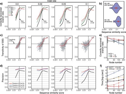
Performance of the GS method in evolutionary simulations. a) Correctly recovered branch ratios of GS and existing methods against average sequence similarity scores. Colored lines are the LOWESS curves (solid black, NJ using MSA-with-complete-gap-deletion; dashed black, NJ using MSA-with-pairwise-gap-deletion; dotted black, NJ using pairwise-sequence-alignment; blue, ML; green, MP; gray, BI; red, GS). Note that the ML, MP, BI and NJ|$_{{\rm MSA}\_{\rm p}}$| lines are heavily overlapped. The vertical lines indicate the average sequence similarity score thresholds where the GS method outperformed the other methods (through c to d). SSS, sequence similarity score. b) Average sequence similarity scores of protein families for which the GS method reconstructed phylogenetic trees with more supported branches (EP values |$\ge $|0.9) than the NJ|$_{{\rm MSA}\_{\rm p}}$| method did (bootstrap values |$\ge $|0.8) (top) and those of the other protein families (bottom). The 243 protein superfamilies data set in total was obtained from the SCOPe database. The violin plots, red points, and gray boxes are the distributions, averages, and standard deviations, respectively. c) Transitivity of SSG against average sequence similarity scores. The gray plots and red lines are the calculated transitivities and LOWESS curves, respectively. The horizontal lines indicate the transitivities where the GS method outperformed the other methods regardless of the indel rate. d) Precision of branches estimated by the GS method under different thresholds of EP values. The colored lines are LOWESS curves of precisions of branches with EP values |$\ge $|0.9 (red), 0.8 (blue), or 0.0 (i.e., all branches, black). e) Correctly recovered branch ratios of the GS and existing methods for different tree sizes. The error bars are standard deviations. For NJ trees, only the one built using pairwise alignment is shown because it performed best. f) Computational times for different tree sizes. The error bars are standard deviations. Dotted purple, MAFFT; dotted orange, all-to-all MMSeqs2; dotted black, NJ with bootstrap analysis (100 replications); and dotted red, GS with EP analysis (100 replications).
![Performance of the GS method in the face of typical problems such as biased taxon sampling (a–c), heterogeneous evolutionary rates (d–f), and long-branch attraction (g–i). a) Schematic figure showing how 32 taxa were selected from a 64-taxon balanced tree for topologies 1–7. Topology 8 was a complete pectinate tree. b) Dendrograms of the topologies 1–7. c) Performance of the GS method in evolutionary simulation under biased taxon sampling (indel rate = 0.02). Violin plots are distributions of correctly recovered branch ratios at different tree topologies (for detailed results, see Supplementary Fig. S7 available on Dryad). Orange, NJ using MSA-with-complete-gap-deletion; yellow, NJ using MSA-with-pairwise-gap-deletion; black, NJ using pairwise-sequence-alignment; blue, ML method; green, MP method; gray, BI method; red, GS method. d) Dendrogram of a 32-taxon tree. The length of each branch ($a)$ was randomly determined based on the normal distribution (mean = 0.5, SD = 0.0, 0.2, 0.5, or 1.0). e) Examples of generated trees at different standard deviation parameters. f) Performance of the GS method in evolutionary simulation under heterogeneous evolutionary rates (indel rate = 0.02). Violin plots are distributions of correctly recovered branch ratios at different SDs (for detailed results, see Supplementary Fig. S8 available on Dryad). g) A phylogenetic tree with two long branches. h) Examples of generated trees at different branch length ratios between the long and normal branches. i) Performance of the GS method in evolutionary simulation under long-branch attraction (in accuracy of the entire tree reconstruction; indel rate = 0.02, branch length [$a$] = 0.5). Violin plots are distributions of correctly recovered branch ratios at different branch length ratios (for detailed results, see Supplementary Fig. S10 available on Dryad).](https://oup.silverchair-cdn.com/oup/backfile/Content_public/Journal/sysbio/69/2/10.1093_sysbio_syz049/1/m_syz049f4.jpeg?Expires=1750199125&Signature=g3QUDiJhxIJBY-ck5F4O7bRSQF-3tlVcSN9gwCDQvn0hZX1BKYvIlKTYqhoRVK7Gl~cVupqInPNW5rveh1YtqFY4tzRSD1PIusylBrWNS~B1-JhQQLQb0VxuBgSBaBbg9YoRJX09IHAID3QDWTozGo-2w9NSNzKRHwxGTWFuCMhnZ4SduEFfMpX4fngbxukw4Tp0xJtdw-BbDzt2-6V4oX25UZ~I1aaI2Kkt7UNSIEjYpw-qh4LtQ1~QuaxtFYEiKoR8y-H5PVVP3VSwezlWwQa1LhWAcv6aNX0Ia7G1euT4FS5p8fsYFIe6AQqaVxMUFUR59hzcznPb-qU3-LO15w__&Key-Pair-Id=APKAIE5G5CRDK6RD3PGA)
Performance of the GS method in the face of typical problems such as biased taxon sampling (a–c), heterogeneous evolutionary rates (d–f), and long-branch attraction (g–i). a) Schematic figure showing how 32 taxa were selected from a 64-taxon balanced tree for topologies 1–7. Topology 8 was a complete pectinate tree. b) Dendrograms of the topologies 1–7. c) Performance of the GS method in evolutionary simulation under biased taxon sampling (indel rate = 0.02). Violin plots are distributions of correctly recovered branch ratios at different tree topologies (for detailed results, see Supplementary Fig. S7 available on Dryad). Orange, NJ using MSA-with-complete-gap-deletion; yellow, NJ using MSA-with-pairwise-gap-deletion; black, NJ using pairwise-sequence-alignment; blue, ML method; green, MP method; gray, BI method; red, GS method. d) Dendrogram of a 32-taxon tree. The length of each branch (|$a)$| was randomly determined based on the normal distribution (mean = 0.5, SD = 0.0, 0.2, 0.5, or 1.0). e) Examples of generated trees at different standard deviation parameters. f) Performance of the GS method in evolutionary simulation under heterogeneous evolutionary rates (indel rate = 0.02). Violin plots are distributions of correctly recovered branch ratios at different SDs (for detailed results, see Supplementary Fig. S8 available on Dryad). g) A phylogenetic tree with two long branches. h) Examples of generated trees at different branch length ratios between the long and normal branches. i) Performance of the GS method in evolutionary simulation under long-branch attraction (in accuracy of the entire tree reconstruction; indel rate = 0.02, branch length [|$a$|] = 0.5). Violin plots are distributions of correctly recovered branch ratios at different branch length ratios (for detailed results, see Supplementary Fig. S10 available on Dryad).
Additional evolutionary simulation with trees that had 50, 100, and 200 nodes also showed that the GS method outperformed the other methods especially for larger trees (Fig. 3e). Finally, the computational times required for phylogenetic analyses using the GS and EP methods are smaller than NJ-method-based approaches and much smaller than those required for ML- and BI-method-based approaches (Fig. 3f).
Finally, we compared the GS method with an existing PSA-based phylogenetic method, PhyPA (Xia 2016), regarding accuracy (including that on diverged sequences) and computational speed using the same simulation procedures. Because PhyPA is a GUI tool, comparison was conducted independently and not thoroughly. While their accuracies were comparable, the GS method ran much faster than PhyPA (0.1 s compared to 2.5 min in case of 24 nodes) (Supplementary Fig. S4, available on Dryad).
The GS Method Is Robust to Major Problems in Phylogenetics
Further simulations were conducted to address major problems in phylogenetic analysis: biased taxon sampling, heterogeneous evolutionary rates, and long-branch attraction. To address biased taxon sampling, eight tree topologies that represented different levels of taxon sampling biases were tested using the same evolutionary simulation framework (Fig. 4a, b). The performance of the GS method was nearly unaffected by the biases and was better than the other methods, especially when the indel rates and branch lengths were large (Fig. 4c and Supplementary S7 available on Dryad). For the second factor, we tested different perturbations to the evolutionary rates in the simulations (Fig. 4d, e). Although strong perturbations worsened the performance of every method, the GS method was the best if the indel rates and branch lengths were large (Fig. 4f and Supplementary S8 available on Dryad). For the last factor, trees with two long branches were considered (Fig. 4g, h). According to the theory of long-branch attraction, those two long branches tend to become close to each other in reconstructed trees (Bergsten 2005). In the simulation analyses, GS method showed similar or less signs of long-branch attraction compared to the other methods (Supplementary Fig. S9 available on Dryad), whereas its performance in accurately reconstructing the entire tree topology was much better than the other methods (Fig. 4i and Supplementary S10 available on Dryad).
The GS Tree of TIM-Barrel Superfamily Proteins Shows Consistency With Their 3D Structures and Suggests Their Early History
As an empirical data set, we applied the GS method to the TIM-barrel superfamily (Copley and Bork 2000), one of the largest superfamilies that contain proteins with diverse and important enzymatic functions and whose “backbone” phylogeny is still under debate (Nagano et al. 2002; Goldman et al. 2016). The sequences of 72 TIM-barrel proteins across the three domains of life were downloaded from the SCOP database (Andreeva et al. 2014), and a phylogenetic tree (GS tree) was reconstructed using the GS method (Fig. 5a). Proteins of similar enzymatic function were properly clustered in the GS tree, and the EP values of many branches were greater than 0.9, showing high statistical robustness. The BI method was also applied to this data set to reconstruct another phylogenetic tree (BI tree), and most of the tree’s branches were supported by small posterior probabilities (Fig. 5b). Specifically, there were several notable topological discrepancies between the GS and BI trees (Fig. 5c). For example, dihydroorotate (DHO) dehydrogenases formed a single cluster in the GS tree but were split into three clusters in the BI tree. To evaluate which topology is more likely, we examined protein 3D structure data, which should reflect the distant evolutionary relationships more sensitively than the primary amino-acid sequences (Thornton et al. 1999). By quantifying structural similarities by RMSDs (Kabsch 1978) and TM-scores (Zhang and Skolnick 2004), we found that proteins with similar structures were more significantly clustered within the GS tree than the BI tree (|$p = 1.55$|e|$^{-9}$| and 5.50e|$^{-10}$| for RMSD and TM-score, respectively; two-sided Wilcoxon rank-sum test) (Fig. 6a). As a typical example, we examined structures of DHO dehydrogenases, dihydropyrimidine (DPY) dehydrogenases, and glutamate synthases (Fig. 6b and Supplementary Movie S1 available on Dryad). Consistent with the GS tree, the structural alignment supported a close relationship between the DHO and DPY dehydrogenases (RMSD 2.81 Å, TM-score 0.78), closer than the relationship between DHO dehydrogenases and glutamate synthases (RMSD 3.71 Å, TM-score 0.59). Secondary structural analysis also supported a closer relationship between DHO and DPY dehydrogenases (Supplementary Fig. S11 available on Dryad). Another example was a specific group of flavin oxidoreductases (denoted by Flavin oxidoreductases [Group 1] in Fig. 5), whose positions were very different in the GS and BI trees. Again, consistent with the GS tree, the structural alignment supported a closer relationship to DHO dehydrogenases (RMSD 3.36 Å, TM-score 0.62) than to another group of flavin oxidoreductases (RMSD 3.64 Å, TM-score 0.68) (Fig. 6c and Supplementary Movie S2 available on Dryad). This result suggests that those two groups of flavin oxidoreductases likely originated independently, and their secondary structures actually show differences (Supplementary Fig. S11 available on Dryad). A comparison to the NJ|$_{{\rm MSA}\_{\rm p}}$|, ML, and MP methods also showed that the GS tree better reflects the structural similarities overall (Supplementary Figs. S12–S14 available on Dryad).
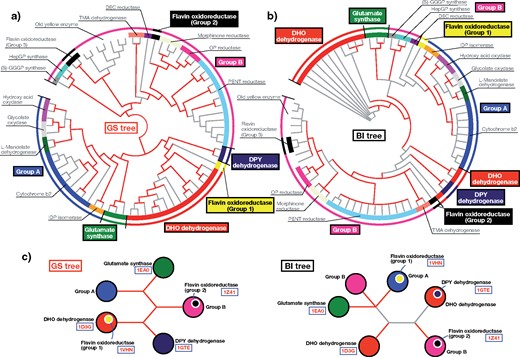
Application of the GS method to TIM-barrel superfamily proteins. a) Phylogenetic tree of TIM-barrel superfamily proteins reconstructed using the GS method. The red branches are those supported by large EP values (|$\ge $|0.9). The inner circle represents functional classes. The outer circle summarizes those classes into several groups for comparison. b) Phylogenetic tree reconstructed using the BI method. The red branches are those supported by large posterior probabilities (|$\ge $| 0.9). c) Summary of topological differences between the GS and BI trees. The PDB IDs of the proteins shown in Figure 6 are presented for reference. (S)-GGGP synthase, (S)-3-O-geranylgeranylglyceryl phosphate synthase; DEC reductase, 2, 4-dienoyl-CoA reductase; DHO dehydrogenase, dihydroorotate dehydrogenase; DPY dehydrogenase, dihydropyrimidine dehydrogenase; HepGP synthase, heptaprenylglyceryl phosphate synthase; IDP isomerase, isopentenyl-diphosphate delta-isomerase; OP reductase, 12-oxophytodienoate reductase; PENT reductase, pentaerythritol tetranitrate reductase; TMA dehydrogenase, trimethylamine dehydrogenase.
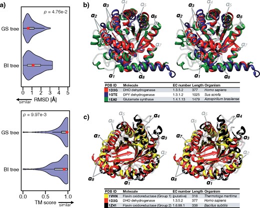
Assessment of the GS tree by 3D structural analysis of TIM-barrel superfamily proteins. a) Violin plots of root-mean-square deviations (top) and TM scores (bottom) averaged over every protein pair in every subtree of the GS and BI trees. The red points and gray boxes indicate the averages and standard deviations, respectively. b) A stereo (parallel) view of 3D structural alignments of a DHO dehydrogenase (red, 4OQV), DPY dehydrogenase (blue, 1GTE) and glutamate synthase (green, 1EA0). Note that |$\alpha $||$_{1}$|–|$\alpha $||$_{8}$| are characteristic alpha-helices of the (|$\beta \alpha $|)|$_{8}$|-barrel structure. Black letters indicate helices that showed particularly large differences in the 3D structural alignment. c) A stereo (parallel) view of 3D structural alignments of flavin oxidoreductase (group 1) (yellow, 1VHN), DHO dehydrogenase (red, 4OQV), and flavin oxidoreductase (group 2) (black, 1Z41).
Discussion
In this era of sequence data deluge, we envision that the GS method will contribute to deciphering the early evolution of various protein superfamilies. In this study, we applied the GS method to the TIM-barrel protein superfamily and obtained a highly resolved phylogenetic tree. DHO and DPY dehydrogenases are involved in pyrimidine biosynthesis. Under the RNA-world hypothesis, protein-mediated pyrimidine biosynthesis is presumed to be one of the most primordial pathways that was needed during a transitional phase from the RNA world to the modern DNA-RNA-protein world (Caetano-Anollés et al. 2007). Both the monophyly of the DHO dehydrogenases and the proximity of the DHO and DPY dehydrogenases would suggest an early appearance of these enzymes with a common origin, consistent with the RNA-world hypothesis. Alternatively, the polyphyly of the flavin oxidoreductases may reflect the universality of flavin as a coenzyme and the importance of oxidation-reduction reactions in various contexts (Walsh and Wencewicz 2013). Although many TIM-barrel proteins are multi-domain proteins and phylogenetic analyses of a single domain cannot decipher the entire evolutionary history of the TIM-barrel protein superfamily, the GS method is a promising scheme for obtaining clues to early evolution of protein superfamilies. To assess how the GS method can be generally applied to other protein superfamilies, we downloaded sequence data from the SCOPe database, which is the extension of the SCOP database and comprehensively and hierarchically classifies proteins by considering structure information. When compared with the NJ trees that are based on the same superfamily data sets, the GS trees have more strongly supported deep branches, which may be further examined using multiple approaches (Fig. 7).
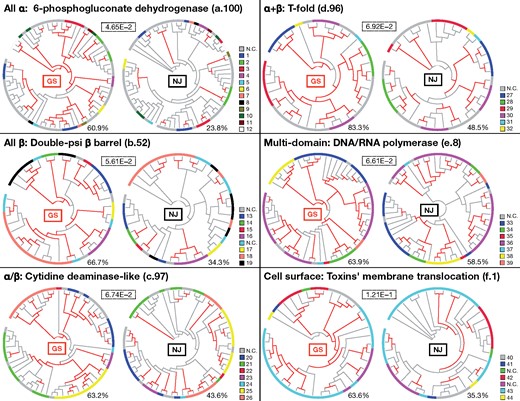
Application of the GS method to protein superfamily data sets obtained from the SCOPe database. Phylogenetic trees of six protein superfamilies were reconstructed using both the GS and NJ|$_{{\rm MSA}\_{\rm p}}$| methods. The red branches of the GS and NJ trees are those supported by large EP (|$\ge $|0.9) and bootstrap (|$\ge $|0.8) values, respectively. The outer circles represent SCOP concise classification strings (functional classes) according to the color legend on each right side (for description, see Supplementary Table S1 available on Dryad). A number in a dotted box indicates an average sequence similarity score of each superfamily proteins. A number below each tree indicates a ratio of interior branches that are supported.
The better performance of the GS method can be regarded as an extension of the previous reports of the good performance of the PSA-based NJ method on data sets that contain remote homologs (Thorne and Kishino 1992; Xia 2016). The reduced performances of the ML, BI, and NJ (except for NJ|$_{\rm PSA})$| methods correlate with the reduced accuracy of MSA (Supplementary Fig. S15 available on Dryad). In addition, the observation that the accuracies of the NJ methods follow the order NJ|$_{\rm PSA} >$| NJ|$_{{\rm MSA}\_{\rm p}} >$| NJ|$_{{\rm MSA}\_{\rm c}}$| also suggests that the deterioration of MSA quality substantially inhibits correct phylogenetic tree reconstruction (Supplementary Fig. S16 available on Dryad) (Xia 2016). Direct comparisons of the alignment accuracies of PSA and MSA were also conducted (Supplementary Fig. S17 available on Dryad). When sequences are substantially diverged, precision of the aligned residues (|$f_{M})$| based on PSA becomes much better than that based on MSA, indicating that MSA tends to “forcibly” align residues too much and introduces substantial noise that impedes downstream analyses. Recall (|$f_{D})$| based on PSA is, in contrast, slightly worse than that based on MSA, probably because information from multiple sequences sometimes helps MSA find correct alignment among several candidates. These results indicate that the former effect is more important than the latter in extracting informative phylogenetic signals from superfamily-scale data sets. It should also be noted that comparisons of the PSA-based and MSA-based GS methods show that the former outperforms the latter, indicating that the algorithm also contributes to the accuracy of the GS method (Supplementary Fig. S18 available on Dryad). A change of |$N_{\rm cut}$| to |$M_{\rm cut}$| (Ding et al. 2001) did not have a significant effect on the accuracy of the GS method (data not shown). A notable difference between the GS method and the other methods is that the GS method accepts only protein sequences as input data. In theory, all-to-all PSA and subsequent spectral clustering can also be applied to nucleotide sequences; however, because extracting remote evolutionary information from nucleotide sequences is thought to be difficult (Zhang and Kumar 1997), the GS method is currently optimized for protein sequences.
In addition to elucidation of the early evolution of protein superfamilies, the GS method can also help us solve “modern” problems, such as the extremely rapid molecular evolution of viruses (Clementi et al. 2004), drug-resistant microbes (Baym et al. 2016), and cancer cells (Gerlinger et al. 2014). As another promising application of the GS method, it can improve the performance of MSA methods by providing guide trees that empower their progressive algorithms (Yamada et al. 2016), because the GS method estimates trees without a precalculated MSA. We actually used the GS method to provide guide trees for MAFFT and Clustal |$\Omega $| (Sievers et al. 2011) and observed improvement in MSA qualities (Fig. 8a). This improvement as guide trees for MSA was similarly observed when PhyPA (Xia 2016) was used if computational speed was ignored (Supplementary Fig. S19 available on Dryad); thus, PSA-based phylogenetic methods can improve MSA performance. Furthermore, the GS method can provide the ML and BI methods with initial trees, which serve as promising starting points for efficiently searching a large space of tree topologies (Ronquist et al. 2012; Stamatakis 2014). Although we did not observe significant improvement in the ML and BI methods using GS-based initial trees, we did find that using MSA with a GS-based guide tree improves performance (Fig. 8b). Because GS trees reconstruct tree topologies without estimating branch lengths, combining GS and ML or BI methods are expected to be especially effective if branch lengths need to be estimated. We have provided a web server for running the GS and EP methods and for downloading the program source codes: http://gs.bs.s.u-tokyo.ac.jp/ and https://github.com/MotomuMatsui.
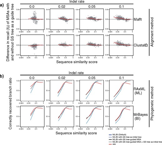
Effects of providing GS tree for phylogenetics as guide and initial trees. a) Effects of providing GS trees as guide trees for MSA. The |$x$|-axis represents average sequence similarity scores. The |$y$|-axis represents differences in accuracies of MSA with and without a GS tree as a guide tree (measured by |$f_{D})$|. Red lines are LOWESS curves. b) Effects of providing GS trees as initial trees in the ML and BI methods. LOWESS curves of correctly recovered branch ratios of phylogenetic trees are plotted against average sequence similarity scores. For the ML (top) and BI (bottom) methods, reconstruction was performed using the default method (blue), using a GS tree as an initial tree (dashed blue), using a GS-tree-guided MSA (black), and using a GS tree as an initial tree and a GS-tree-guided MSA (dashed black). For comparison, the results of the GS method are also shown (red).
Supplementary Material
Data available from the Dryad Digital Repository: http://dx.doi.org/10.5061/dryad.ps0qf4r.
Funding
This work was supported by the Japan Society for the Promotion of Science [15J07743, 16H06154, 17H05834, 18H02493, 18H04136, and 17K07509], the Ministry of Education, Culture, Sports, Science and Technology in Japan [221S0002 and 16H06279], and the Canon Foundation.
Acknowledgments
The authors thank members of the Iwasaki laboratory, the editor, and three anonymous reviewers for helpful comments on this research. Computations were partially performed on the NIG supercomputer at the ROIS National Institute of Genetics and the SuperComputer System, Institute for Chemical Research, Kyoto University. The GS method source code and web server are freely available at the project web site (http://gs.bs.s.u-tokyo.ac.jp/).
