


Abstract
We examine how different spatial compositions affect the educational achievement in mathematics of 16-year-old students in Chile, a Latin American country with high inequality and one of the most segregated education systems in the world. Conceptually, we complement the literature on ‘neighbourhood effects’, which typically addresses the influence of concentrated disadvantage, by focusing on concentrated advantage and its influence on educational outcomes. We construct a panel with all school students who took a national standardized mathematics test in 2010, 2014 and 2016 in the Metropolitan Region of Santiago, Chile. We complement it with survey data for the 52 districts of the Metropolitan Region, clustering the districts based on factors such as unemployment, economic inequality, access to services, experiences of violence and stigmatization. Our different identification strategies consistently show that concentrated poverty and affluence are both relevant for explaining educational achievement in mathematics above and beyond individual and school characteristics.
1. Introduction
The spatial dimension of economic inequality has gained scientific relevance in explaining people’s life opportunities (e.g. Wilson, 1987; Jencks and Mayer, 1990; van Ham et al., 2012; Sharkey and Faber, 2014). A large part of the so-called ‘neighbourhood effects’ literature has focused on studying the influence of residential disadvantage on several educational outcomes including school dropout, level of instruction and standardized test performance (see Nieuwenhuis and Hooimeijer (2016) for a recent review). Studies have found mixed evidence in this regard, often reporting small effects and sometimes even no significant effects at all (e.g. Brooks-Gunn et al., 1993; Bramley and Karley, 2007; Ainsworth, 2010; Owens, 2010; Sharkey, 2010; Wodtke et al., 2011; Caudillo and Torche, 2014; Otero et al., 2017; Wodtke and Parbst, 2017; Howell, 2019; Nieuwenhuis et al., 2019). As such, the potential impact of residential conditions on educational outcomes has been intensely debated, especially due to methodological imperfections but also conceptual aspects.
In terms of conceptual issues, questions have arisen regarding the delineation of scales at which processes take place and the variety of mechanisms that might drive neighbourhood effects (e.g. Galster, 2012; Sharkey and Faber, 2014). Methodologically, there are discussions relating to the heterogeneity of neighbourhood effects (e.g. Galster et al., 2010; Wodtke et al., 2016), the timing and duration of exposure to residential environments (e.g. Wodtke et al., 2011; Musterd et al., 2012), the potential nonlinear shape of neighbourhood effects (e.g. Galster et al., 2015; Galster, 2018), the bias of omitted variables associated with household and school contexts (e.g. Nieuwenhuis and Hooimeijer, 2016; Nieuwenhuis et al., 2019) and the relevance of concentrated advantage for explaining educational outcomes (e.g. Johnson, 2013; Toft and Ljunggren, 2016; Howell, 2019). In this paper, we focus on addressing some of these issues.
The first issue is the relative importance of concentrated affluence. Scholars have proposed a range of theoretical mechanisms through which living in disadvantaged neighbourhoods may affect various outcomes. For instance, collective socialization, neighbourhood cohesion and exposure to violence (see Galster (2012) for an overview). However, examination of how the problems experienced by the most marginalized result in greater educational inequality requires additional reflection upon the privileges of the most advantaged (Toft and Ljunggren, 2016). Some scholars have argued that areas of affluence are likely to be a stronger contributor to educational outcomes than concentrations of poverty (Johnson, 2013). Nevertheless, little is currently known about how living in affluent areas may influence such outcomes, that is the potential mechanisms of action (cf., Brooks-Gunn et al., 1993; Leventhal and Brooks-Gunn, 2000; Howell, 2019). To shed light on this issue, the present study enriches the conceptualization of advantaged neighbourhoods and identifies the kind of mechanism that may theoretically channel the effect of concentrated affluence onto educational outcomes, thus generating further advantage.
The second issue concerns the asymmetrical forms of causation with regard to spatial context. Researchers have based their analyses of the workings of spatial disadvantage on educational outcomes, using several measures to represent the underlying mechanisms, including factors such as neighbourhood poverty, unemployment level, criminal activity, the proportion of migrant/ethnic groups and a lack of access to public services (Nieuwenhuis and Hooimeijer, 2016). However, the different ways in which these spatial characteristics truly operate to affect educational outcomes is still unclear (e.g. Harding, 2011; Sharkey and Faber, 2014). This analytical shortcoming is closely related to two empirical weaknesses: (1) the spatial characteristics used to represent the explanatory principles have rarely been combined in research in order to understand their intersectionalities and (2) few studies have explicitly examined the potential nonlinear and threshold aspects of neighbourhood effects (e.g. see Galster (2018) for an overview). To help alleviate these issues, we focus on representing the spatial structure, that is the various spatial areas that are observable according to a number of characteristics (e.g. income levels, economic inequality and access to services). We then determine the distinctive effect of these spatial configurations on academic achievement.
The third issue relates to the relevance of school context for neighbourhood effects studies. Most studies have focused on testing how spatial characteristics influence educational outcomes after considering students’ socio-economic background. Nevertheless, the school context may also play a relevant role in explanations of school learning, especially given the multiple resources offered by institutions and their particular decisions and practices (Bronfenbrenner, 1979). Joint analysis of these contexts has proved relevant in empirical terms, especially for reducing the omitted variable bias (Nieuwenhuis and Hooimeijer, 2016). Residential segregation appears to play an important role here: studies that have found that neighbourhood conditions predict academic outcomes even after controlling for school characteristics have been conducted, to a great extent, in contexts with relatively pronounced levels of residential segregation, such as Latin America, the UK and the USA (e.g. Owens, 2010; Otero et al., 2017; Wodtke and Parbst, 2017; Nieuwenhuis et al., 2019). Therefore, we jointly test the relevance of school and spatial contexts on academic achievement. We also consider previous individual educational attainment in order to identify more reliable neighbourhood effects.
Against this background, the present study examines the effect of different spatial configurations on mathematics achievement among adolescents. Our inquiry focuses on Chile, a middle-high-income Latin American country with one of the most unequal income distributions in the world. We specifically analyse the Metropolitan Region of Santiago, a highly segregated city and home to nearly 40% of the national population. Our research question reads as follows: To what extent do different spatial compositions (especially concentrated poverty and wealth) predict the academic achievement of Chilean students in mathematics above and beyond family background, school context and individual characteristics?
To answer this question, we used a sample of 50 265 10th graders (aged 15–16 years). We took a panel of administrative data that include information about student performance in a standardized mathematics test, along with household and school characteristics, and combined it with additional survey data providing aggregate information for the 52 districts of the Metropolitan Region of Santiago, Chile.
2. Theoretical background
2.1 Spatial segregation and educational inequality
When trying to understand differences in educational outcomes generated by spatial context, residential segregation is key. Segregation is the spatial expression of economic inequality and refers to the extreme residential concentration of socio-economic groups (Marcuse, 2005). At the macro level, residential segregation is assumed to be the result of advanced large-scale processes of housing commodification involving the increasingly high cost of land, the speculative interests of private developers and the marketization of social housing (e.g. Slater, 2013). Residential segregation is also arguably reinforced by self-selection at the top of the spatial structure, that is, due to the preferences of the upper strata to promote a kind of spatial differentiation and reside among ‘equals’ (see also Massey (1996) and Atkinson and Blandy (2006)).
Residential segregation driven by processes of urban neoliberalization and emerging self-segregation of the wealthy has tended to broaden gaps between the upper and lower classes, especially in the Global South. In Chile, for instance, segregation according to socio-economic status (SES) is now much intense than in the welfare regimes typically found in Western Europe (Agostini et al., 2016). In this context, the affluent might increase their privileges through space, whereas people with scarce capital are likely to be affected by two-pronged exclusion: spatial fixation in vulnerable areas and limited urban accessibility, which in turn increases their disadvantage (see also Otero et al., 2021). This points to spatial inequality as a relational problem whose analysis should consider residential characteristics at both ends of the spatial continuum, especially the privileges enjoyed by those who occupy higher positions within class and spatial structures. Affluent residential areas can, for instance, facilitate educational inequality and the intergenerational transmission of socio-economic advantage by reinforcing positive socialization of students and providing helpful social networks, along with the resources and support needed to comply with school requirements (e.g. Leventhal and Brooks-Gunn, 2000; Johnson, 2013; Howell, 2019). In the following sections, we elaborate further on how segregation, expressed through concentrated poverty and wealth, might foster differential educational achievement at both ends of the spatial spectrum.
2.2 The mainstream mechanisms of neighbourhood effects on educational outcomes
Theoretically, scholars studying ‘neighbourhood effects’ have posited that concentrated disadvantage negatively influences educational outcomes through four main mechanisms: social isolation, social disorganization, lack of institutional resources and environmental hazards.
Social isolation theories suggest that residents of impoverished residential areas are disconnected from the social networks of the middle classes and traditional institutions (Wilson, 1987). It is argued that this generates major obstacles in the socialization processes of children and adolescents, in particular with regard to the stimulation of academic success at school and conveying the advantages of formal education (Jencks and Mayer, 1990; Leventhal and Brooks-Gunn, 2000; Ainsworth, 2010). Other scholars have noted that concentrated disadvantage negatively impacts educational outcomes due to the presence of heterogeneous (competitive and conflictive) cultural models of schooling, which include both ‘middle-class’ dispositions and orientations associated with ‘alternative’ cultures (Harding, 2007). In this context, it is presumed that students have fewer opportunities to act consistently with the aims that they express regarding their educational and occupational future. They may also find it easier to change their path if their social environment provides them with other choices (see also Harding, 2011).
Explanations associated with social disorganization have focused on the internal processes of neighbourhoods. In general, it is assumed that residents of disadvantaged residential areas encounter difficulties in the formation and maintenance of supportive networks and local cohesion (e.g. Sampson et al., 1997; Morenoff et al., 2001). As such, residents experience barriers to closer supervision of children and implement informal social controls in an attempt to reduce potential negative dispositions towards education (see also Leventhal and Brooks-Gunn, 2000). Alternatively, although residents may have plenty of social ties within the neighbourhood, these connections probably do not involve the same social power and prestige as those in more affluent places (e.g. Marques, 2015). Consequently, parents likely find it difficult to challenge the authorities and request better educational facilities, which logically can affect students’ performance.
Scholars who have focused on institutional resources suggest that ‘neighbourhood effects’ are driven by the quality of the services available in residential areas. It is noted that concentrated disadvantage goes hand in hand with lack of access to supermarkets, green areas, healthcare and cultural facilities (Wilson, 1987). Specifically, schools located in marginalized residential areas often encounter serious budgetary obstacles to acquisition of teaching resources, the hiring of highly qualified teachers and the implementation of support programmes (Small and Newman, 2001). In this context, students’ educational aspirations and skills for achieving their academic goals can be severely affected (e.g. Bramley and Karley, 2007; Ainsworth, 2010).
Environmental theories of neighbourhood highlight area-based inequality in exposure to contaminants. It is argued that the most impoverished areas of cities are usually located near motorways, waste sites and manufacturing facilities, and therefore tend to exhibit higher levels of air and water pollution, ambient noise and heavy metals. These problems may be especially harmful to child development (Crowder and Downey, 2010). Children and adolescents living in disadvantaged residential areas are also more likely to be overexposed to dwellings that have fallen into disrepair, which can severely affect their health condition due to the presence of toxins. Indeed, these environmental hazards can lead to a number of diseases, respiratory problems, allergies and mental stress, increasing students’ school absenteeism and thereby decreasing their cognitive skills and educational achievement (e.g. Mohai et al., 2011; Chen et al., 2018).
Another relevant channel through which environmental constraints can affect students’ performance is exposure to violence. There is often a higher risk of criminal behaviour in disadvantaged neighbourhoods, meaning that students are more likely to witness, for instance, a shooting or a stabbing or be threatened with a weapon (Harding, 2009). Direct and indirect exposure to violent situations may be particularly damaging to the cognitive functioning and academic performance of children and adolescents (e.g. Sharkey, 2010; Caudillo and Torche, 2014). In this case, the particular mechanisms associated with poor academic outcomes can involve psychological and motor symptoms, such as post-traumatic stress disorder, experiences of fear, anxiety and depression, and speech impediments (see also Sharkey and Faber, 2014).
Beyond this theoretical core, other complementary mechanisms suggested in the literature include residential stigma and relative deprivation. With regard to the former, scholars have suggested that qualified teachers might not be available to work in schools located in stigmatized residential areas or districts, which can lead local students to receive lower quality education and undervalue educational achievement (e.g. Galster, 2007). With regard to the second mechanism, it is expected that visible economic inequalities and, in particular, polarization within a residential environment may have a negative impact on educational outcomes (e.g. Otero et al., 2017). In part, this can be due to increased distress and status frustration.
2.3 Understanding the ‘privilege’ of those living in wealthy areas in order to explain better educational outcomes
In general, we posit that living in affluent areas may provide further opportunities for the privileged to achieve desirable educational goals. This is precisely the point made by scholars concerned with the schooling and residential strategies of the upper-middle classes in several Latin American and European cities (e.g. Andreotti et al., 2015; Bacqué et al., 2015; Méndez and Gayo, 2019), who have suggested that the upper-middle classes operate to a great extent as social ‘segregators’—as a group that aspires to live ‘among equals’ in order to accumulate different resources and facilitate social reproduction or upwards social mobility for their children. We propose that concentrated advantage may positively affect educational outcomes through three main mechanisms: desirable role models, social cohesion and institutional resources.
The preference of the upper classes for living among ‘equals’ in affluent residential environments has major implications for young people’s collective socialization. When it comes to educational aspirations, residents of affluent areas are expected to be much more homogeneous than those living in other residential environments and to comply with the expectation of completing a bachelor’s degree or higher qualification (Harding, 2011). This value homogeneity might be explained by the type of parenting commonly promoted within privileged groups. Upper-class nurturing more often adheres to what Lareau (2011) calls ‘concerted cultivation’, which tends to be focused on the development of children’s talents and skills. Students are encouraged, for instance, to participate in socio-cultural extracurricular activities in their free time, which arguably increases their motivation and confidence to tackle educational demands. This type of cultural orientation is often widespread within affluent residential environments, so it is expected to reinforce a positive collective socialization towards education (e.g. Lareau and Goyette, 2014).
The experience of living in affluent segregated neighbourhoods can also provide substantial advantages in terms of cementing stronger neighbourhood cohesion, such as place attachment, networked pragmatism and performative practices of place-making (e.g. Savage et al., 2005). Although this type of local togetherness can operate as a form of ‘collective efficacy’ to tackle crime and antisocial behaviours, it mostly represents a set of attitudes focused on working for the neighbourhood and improving residential conditions in a broader sense (e.g. Maloutas and Pantelidou Malouta, 2004; Méndez and Gayo, 2019). As such, neighbourhood cohesion may be understood in part as an instrument that residents of affluent segregated areas can use to increase their class privileges (see also Méndez et al., 2020). When applied to education, neighbourhood cohesion can be helpful in the creation and maintenance of networks of social support in various issues regarding parental involvement and other school demands. It is also expected to increase positive influence among students, since they are more likely to spend time together. In short, affluent segregated areas can be conducive to supportive ties and further normative pressures on students to achieve better academic performance (e.g. Toft and Ljunggren, 2016; Howell, 2019).
It is also common for affluent segregated areas to exhibit a greater endowment of institutional resources when compared with other residential configurations. Indeed, these environments typically have more green spaces and cultural facilities (e.g. museums, theatres and libraries), as well as better public schools (see also Bacqué et al., 2015). Parents who can afford to reside in affluent areas move to such places precisely in order to enjoy access to high-quality institutional resources (Butler and Hamnett, 2007). These pragmatic advantages allow upper-class residents to support their class sociability in a variety of social settings and increase their general wellbeing (Lareau and Goyette, 2014). More importantly, provision of good healthcare for students can result in better child development, while access to privileged educational infrastructure and facilities arguably provides better support for students to achieve educational success (e.g. Leventhal and Brooks-Gunn, 2000; Johnson, 2013).
2.4 Research site and hypotheses
Since the establishment of neoliberal rule in Chile during the military dictatorship (1973–1990), the political economy has been developed within the framework of a subsidiary state (Taylor, 2003). Radical privatization reforms to education and housing have increased class inequality (see e.g. Otero et al., 2021). With regard to the education system, the Chilean neoliberal model has stimulated strong segregation according to SES (Valenzuela et al., 2014). Wealthy parents can afford expensive tuition fees and enrol their children in fully private schools that constitute around 10% of provision, whereas middle-class and lower-class parents are forced to enrol their children in subsidized private schools and public schools that serve approximately 55% and 35% of all students, respectively (Gayo et al., 2019). This unequal access to educational opportunities has resulted in stark differences in educational achievement by school type. In fact, the highest scores in standardized tests of academic performance have systematically been achieved by private school students due to the capability of these institutions to invest in better infrastructure and highly qualified teachers, which has led to increased opportunities for children from privileged family backgrounds to forge successful trajectories (see also Carrasco and Gunter, 2019).
In parallel to the stratification of the education system, there has been an increase in spatial division according to class, especially in the Metropolitan Region of Santiago, the main urban agglomeration in Chile. Over the last three decades, the state has given up urban planning power and deregulation of the private rental sector has produced higher levels of segregation (see Garreton, 2017). Due to lack of choice and the availability of easily accessible and affordable housing, the lower classes have preserved and even reinforced their location in peripheral districts marked by concentrated poverty, overcrowding, lack of public investment and residential stigma (e.g. Otero et al., 2021), whereas the middle classes have concentrated themselves in newly constructed high-rise developments in more central urban areas characterized by high residential density (e.g. López-Morales, 2016). Simultaneously, the spatial divisions between the top and the rest of the social hierarchy have become particularly strong. There has been a clear progressive self-segregation of upper-middle-class families in the north-eastern part of Greater Santiago, accompanied by a radical increase in land values (Méndez and Gayo, 2019). These residential areas have better provision of goods and services such as schools, cultural facilities and green areas, and have achieved the highest levels of neighbourhood cohesion in terms of place attachment, neighbourly trust and local organization (see also Méndez et al., 2020).
In accordance with our theoretical background, we therefore expect that educational achievement can be explained not only by individual characteristics and type of school but additionally by spatial context. In other words, we expect to see additional reinforcement of educational inequality due to spatial segregation. Specifically, we have argued that both concentrated disadvantage and concentrated affluence should influence educational outcomes through different mechanisms. In the Metropolitan Region of Santiago, the spatial divisions of poverty and wealth are particularly visible and might be reinforcing the well-established class inequality associated with family backgrounds and the segregation of the education system. In addition, it is possible that the growing preference for self-segregation among the privileged make neighbourhood effects especially strong at the top compared with the bottom of the spatial structure. After all, it is already clear that the region has become a more unequal place with a marked increase in concentrated affluence.
The following hypotheses are derived from the above discussion:
Hypothesis 1: Spatial context will affect academic performance, even accounting for individual and school characteristics. In particular, exposure to disadvantaged areas will lead to lower educational achievement (H1a), whereas exposure to advantaged areas will result in higher educational achievement (H1b).
Hypothesis 2: Spatial effects on educational achievement will appear stronger in advantaged than disadvantaged areas. In other words, the positive effect of exposure to affluent areas will be greater than the negative effect of exposure to impoverished areas.
In what follows, we describe the data and methods before discussing our findings.
3. Data
3.1 Data
The present study uses panel data from 50 265 adolescent students who took the Chilean Education Quality Agency [Sistema Nacional de Medición de la Calidad de la Educación, SIMCE] standardized test in mathematics in three different school grades: 4th grade (in 2010), 8th grade (in 2014) and 10th grade (in 2016). The database contains the population of students who take the test in a given year, and each year, test scores are standardized so that they always have a mean close of approximately 250 points and a standard deviation of 50 point. To provide detailed information on district-level characteristics, we use the National Socio-economic Characterisation Survey [Encuesta de Caracterización Socioeconómica Nacional, CASEN]. CASEN is a nationally representative survey that covers a random sample of households based on the national census. We use the 2015 wave, which was the first to be representative at the district level and includes 58 142 households.
We merged the district-level information from CASEN with the SIMCE data. We used school district, as students’ district of residence is not available in the SIMCE data. Fortunately, this is not a substantive problem, as over 80% of students attend schools within the same district in which they reside (see e.g. Otero et al., 2017). In our sample, few students changed districts during their time at school. Around 66% of students remained in the same district between 4th and 10th grade, and 77% remained in the same district between 8th and 10th grade. As such, we can assert that neighbourhood effects are persistent over time.
While we do have information on all students who took the test in 2016, we drop a number of observations in the process of creating our dataset. The final number of observations is the result of a combination of choices and data requirements. Table 1 summarizes this process. As shown, 248 158 students were registered to take the 2016 SIMCE test, of which 96 554 registered in the Metropolitan Region. Within the region, 74 120 students took the test. Furthermore, some of the test-takers’ ID numbers are duplicated in the dataset and do not allow for an accurate merge of the information for the same student across years. We therefore restrict our sample to students for whom we can perform a successful match either through their personal ID or through a combination of personal ID, gender and school ID. 60 081 students are correctly identified and merged across all three years. Of these, 59 298 were also in the Metropolitan Region in 2014 and of these, 50 265 were in the region in 2010 as well. Our final sample accounts for 68% of our ‘target’ population (i.e. students from the Metropolitan Region who took the SIMCE test in 2016), 52% of all students in the region and 20% of all students in the country.
Number of observations
| Number of cases | Share of total | Share of MR | Share of MR test-takers | SIMCE score | Share women | Public school | Subsidized private school | Private school | |
|---|---|---|---|---|---|---|---|---|---|
| Total in 2016 | 248,158 | 100% | – | – | . | 50.2% | 36.3% | 55.5% | 8.1% |
| Studies in metropolitan region (MR) in 2016 | 96,554 | 38.9% | 100% | – | . | 50.1% | 24.2% | 62.7% | 13.1% |
| Took SIMCE 2016 test | 74,120 | 29.9% | 76.8% | 100% | 272.7 | 49.3% | 20.9% | 65.2% | 13.9% |
| Correctly merged students | 60,081 | 24.2% | 62.2% | 81.1% | 279.0 | 50.1% | 19.1% | 66.1% | 14.8% |
| Studies in MR in 2014–2016 | 59,298 | 23.9% | 61.4% | 80.0% | 279.2 | 50.1% | 19.0% | 66.2% | 14.8% |
| Studies in MR in 2010–2016 | 50,265 | 20.3% | 52.1% | 67.8% | 283.7 | 51.1% | 18.5% | 66.2% | 15.4% |
Table 1 includes the average test score at each step of the process, as well as other covariates. Average scores increase in size as we restrict the number of observations, from 272.2 to 283.6 points. Overall, this is a small increment of just above 20% of a standard deviation. Although the average score increases, it is safe to say that the overall composition of our final sample does not change substantially from that of our target population. Similarly, the gender and type of schools distributions remain relatively unchanged when focusing in the Metropolitan Region.
Our dataset includes the population of students who took the SIMCE test in the Metropolitan Region in 2010, 2014 and 2016. As such, our focus will be placed on the estimated coefficients rather than statistical inference. However, for transparency, we report standard errors for all estimations, and we provide robustness checks aimed at correcting them when necessary. Using education research for the USA as an example, Gibbs et al. (2017) argue that the use of statistical inference can result in mistaken conclusions when using administrative data, as statistically insignificant estimates can be disregarded despite having ‘substantive’ significance. For that reason, despite including standard errors and P-values, most of our discussion will be based on the sign and size of our estimates.
4. Variables
4.1 Dependent variables
Our variable of interest is the mathematics score of 10th grade students. We build three dependent variables that allow us to explain not only average educational achievement but its distribution across students:
10th grade mathematics score.
Scoring within the top 25% (binary).
Scoring within the bottom 25% (binary).
4.2 Measuring the spatial context
We examine the Metropolitan Region of Santiago, Chile. The region is divided into 52 districts and contains about 40% of the national population—about 7 million inhabitants. We focused on this region not only because it is the most important urban agglomeration in the country but, more importantly, because it clearly reflects the extreme economic inequality of Chile.
Our analyses are focused on the district scale, as it most clearly represents the spatial segregation found in Santiago. In fact, it could be said that spatial inequality is produced to a certain extent by district-scale differences in terms of the financial resources that districts are able to collect through the payment of commercial licences, land tax and other permits and licences. The difference in the financial resources available for districts to spend on security services, cleaning, lighting and street paving is stark. In wealthy districts such as Las Condes, Providencia and Vitacura, local authorities have a per-resident budget of around US$1500 a year, while those of poorer districts like Cerro Navia and El Bosque have only around US$200 per inhabitant. This is in addition to income from healthcare and education services.
We propose a holistic characterization of students’ surroundings. Instead of separately examining the effect of each spatial characteristic on academic performance, we sought to represent spatial clusters of districts with shared characteristics through principal components and clustering methods. The benefits of using a cluster approach are both theoretical and empirical. Although we lose the capacity to account for separate effects, say, to compare the effect of the unemployment rate with access to services, we gain the ability to identify homogeneous areas on an informational basis, especially the spatial divisions of poverty and wealth underlined in our theoretical background. It also enables us to better account for the high correlation between the multiple district characteristics, which often results in multicollinearity issues, and focus on how they combine to represent specific areas.
Specifically, we applied hierarchical clustering on principal components (HCPC). Here, different principal components methods are used as a pre-procedure in order to facilitate a more reliable clustering solution later (see Husson et al., 2011). In our case, the first step of the HCPC approach is a principal component analysis (PCA) to reduce the georeferenced (continuous) data to a smaller set of dimensions. We used 28 spatial characteristics including poverty rate, income inequality and access to green spaces and services (see Table 1). In our analysis, the first two principal components explain 64.4% of the total variance, which is an acceptable portion (Abdi and Williams, 2010). The second step of the HCPC approach uses hierarchical clustering according to Ward’s criterion on the two selected principal components. The last step uses k-means clustering to improve the previous partition. Based on these analyses, we arrived at a six-spatial-cluster solution, with noteworthy differences among groups.
Table 2 briefly describes the spatial clusters identified and Table 2 presents more detailed information regarding the distribution of spatial characteristics between spatial clusters. Similarly, Table 3 highlights the most distinctive differences between spatial clusters by including those variables with the highest departures from the mean. For instance, Cluster 1 has above-average experiences of shootings and fights as well as below-average levels of education. Cluster 6, on the other hand, has higher levels of income and education, and lower levels of fights, trash or plagues.
Summary of spatial clusters
| % | Description | |
|---|---|---|
| Cluster 1 | 17.3% | Low-income districts, with low economic inequality and a low educational level. Also characterized by experiences of violence (e.g. fights, shootings and drug consumption). This cluster comprises 13 districts, including El Bosque, La Pintana, Lo Espejo and Pudahuel. |
| Cluster 2 | 0.5% | Rural districts characterized by low levels of access to services, especially cash machines, supermarkets and community services. High levels of economic polarization. Also characterized by a higher share of people reporting infestations and larger networks. This cluster comprises four districts: Alhue, Calera de Tango, Maria Pinto and San Pedro. |
| Cluster 3 | 13.9% | Rural districts characterized by low levels of access to services, especially parks, educational institutions and pharmacies. High levels of economic polarization. Also characterized by relatively high participation in neighbourhood associations and higher poverty rates. This cluster comprises 12 districts, including Buin, Colina, Pirque and Tiltil. |
| Cluster 4 | 37.8% | Middle-class districts characterized by good access to services such as transport, education and supermarkets. A relatively low level of inequality. It shows a lower share of people with higher education, and relatively low levels of perceived residential stigma. This cluster comprises 14 districts, including Independencia, La Florida, Puente Alto, Quinta Normal and Renca. |
| Cluster 5 | 19.4% | Upper middle-class districts characterized by low levels of poverty and residential stigma. Relatively high levels of economic inequality. Participation in neighbourhood organizations. Acoustic and visual pollution. This cluster comprises five districts: La Reina, Macul, Ñuñoa, San Miguel and Santiago. |
| Cluster 6 | 11.1% | This cluster captures the higher income districts of the Metropolitan Region of Santiago. Also characterized by high levels of education, both in terms of years of schooling and the share of people with tertiary education. Low levels of infestations, trash in public places and fights in the street. It also shows a low poverty rate (less than 1%). This cluster comprises four districts: Las Condes, Lo Barnechea, Providencia and Vitacura. |
Averages for individual and school variables, by cluster
| Cluster 1 | Cluster 2 | Cluster 3 | Cluster 4 | Cluster 5 | Cluster 6 | Total | |
|---|---|---|---|---|---|---|---|
| Students’ characteristics | |||||||
| SIMCE 10th grade | 267.3 | 264.1 | 270.5 | 280.1 | 289.3 | 328.9 | 283.7 |
| SIMCE 8th grade | 265 | 268.5 | 268 | 274.2 | 281.4 | 310.5 | 277.2 |
| SIMCE 4th grade | 274.4 | 277.6 | 279.1 | 280.7 | 290.7 | 307.1 | 284.2 |
| Female | 50.80% | 43.90% | 51.50% | 51.10% | 51.10% | 51.50% | 51.10% |
| School context (type of school) | |||||||
| Public school | 12.60% | 52.00% | 26.70% | 13.40% | 27.10% | 18.00% | 18.50% |
| Subsidized private school | 85.40% | 11.80% | 61.20% | 79.60% | 57.10% | 15.30% | 66.20% |
| Private school | 2.10% | 36.20% | 12.10% | 7.00% | 15.80% | 66.70% | 15.40% |
Figure 1 shows a factor map to represent how the 52 districts of the Metropolitan Region of Santiago are located with respect to the two principal components and their spatial clusters. The first component (dimension 1) makes a clear distinction between districts with poor access to services (clusters 2 and 3, to the left) and districts with medium-good access (clusters 1, 4, 5 and 6, to the right). The second component (dimension 2) shows socio-economic differences, with high-income districts at the top (notably Cluster 6) and poorer districts at the bottom (notably Cluster 1). As shown in Figure 1, Cluster 6 constitutes the most distinct spatial configuration—being the farthest from the rest of the clusters—and clearly represents the condition of living in advantaged areas. In general, the spatial divide identified is visibly consistent with the SES-based spatial segregation patterns reported in previous research focused on the district level (e.g. Agostini et al., 2016; Garreton, 2017).
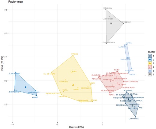
Factor map representing the two principal components and the spatial context (clustered districts).
4.3 Control variables
Our empirical strategy allows us to account for individual-, household- and school-level characteristics. However, we include whether the school is public, subsidized private or fully private in order to control for overarching differences between school type. Individual-level characteristics include gender and SIMCE scores in 4th and 8th grades. Past scores are particularly relevant since they are a central part of our causal identification strategy. Table 3 presents descriptive statistics for individual, household and school variables by cluster and in total.
5. Empirical strategy
To examine how being exposed to a cluster shapes test scores, we need to account for the potential endogeneity between the cluster and test scores. We can group these sources into two categories: time-invariant factors and factors that change over time. The former group includes individual and household characteristics, such as parents’ SES. The latter group includes factors that shape the dynamic aspect of this relationship, such as circumstances that occur ‘along the way’ and require us (or our parents) to adapt and modify our (or their) choices. Estimating the effect of exposure to a particular cluster requires us to control for both sources of bias.
Although several empirical approaches are available for this purpose, the final choice is far from innocuous. Previous research has shown that estimation of neighbourhood effects is highly sensitive to the statistical approaches used to address different sources of bias (see, e.g. Galster and Sharkey, 2017, pp. 13–14). As no single approach addresses all of these issues, the authors argue in favour of a ‘multi-method’ approach to ensure the robustness of estimates. We provide the results for our main approach in the main text while providing multiple robustness checks later in the Online Appendix.
Our main results follow from two identification strategies, the first to account for time-invariant sources of bias and the second to account for dynamic sources. To account for time-invariant sources of bias, fixed effect regressions remain the benchmark when panel data are available. Galster and Hedman (2013) consider fixed effect regression to be among the best approaches to addressing estimation bias, particularly when combined with instrumental variables (given strong and valid instruments). Our data allow us to build a panel dataset of students for three periods of time and thus account for individual and school fixed effects.
Unfortunately, we are unable to complement fixed effect regressions with instrumental variables for two reasons. First, the survey only collects information on household characteristics, which are unlikely to satisfy the exclusion restriction. Second, and perhaps most importantly, the take-up of this survey is not perfect, and using these variables would bias our sample in favour of the most well-off students. While we do not include instrumental variables among our ‘battery’ of estimations, we do consider all other estimation approaches discussed by Galster and Hedman (2013).
To account for dynamic sources of bias, we use a lagged dependent variable estimation (see Ashenfelter and Card, 1985; Bellemare et al., 2017). This approach includes as covariates the same student’s previous test scores. Parents can take action based on previous scores; for example, in the event of a low score, they can decide to move their children to a different school in order to provide a better learning environment. Furthermore, lagged test scores could account for additional parent involvement or investment such as private tutoring if those changes are a result of a previous bad score. Controlling for past scores allows us to account for time-variant factors that cannot be accounted for in standard fixed-effect settings.
Persistence in our spatial clusters is quite high. In our sample, 74% of students remain in the same spatial cluster between 4th and 10th grades, and over 82% do so between 8th and 10th grades. This creates a problem when using a fixed effect estimation. If we were to simultaneously account for spatial clusters and individual fixed effects, we would only estimate the effect for the few students who have changed cluster during our reference period (i.e. between 4th and 10th grades). Conversely, it would be impossible to estimate the effect for the non-movers sample, as the fixed effect encompasses the effect of the cluster. In cases such as these, the standard recommendation is to use an alternative estimation approach, such as random effects. However, as Galster and Hedman (2013) discuss, unobserved time-invariant factors (i.e. those captured by a fixed effects regression) might be a stronger source of selection bias than those captured by a random effects regression.
To account for the fixed effects and for the effect of the spatial clusters, we applied a two-stage process. First, we estimated a fixed effect regression for SIMCE test scores with individual, school and time fixed effects. Second, we estimated the effect of the spatial clusters for a cross-section using the residual from the first stage as our dependent variable. By construction, the residual from the first stage is the SIMCE test score, minus the individual, school and time averages, thus excluding all time-invariant sources of bias.
In the first stage, we estimate a fixed effect regression to account for time-invariant factors that could bias our estimation. For a student i in school , cluster neighbourhood , and time period their standardized score is defined by
where , , and account for individual, school and time fixed effects, respectively.
To account for these fixed effects, we estimate Equation (1) for the three available periods: 4th, 8th and 10th grades. We obtain our dependent variable by subtracting the estimated fixed effects from the standardized test score:
As a result, our dependent variable in all of the following estimations is the residual from Equation (1), that is, the test score clean of individual, school and time averages, as defined in Equation (2).
In the second stage, we estimate the effect of the spatial clusters:
where are individual characteristics in time t, are school characteristics in time t, are district cluster fixed effects, and are standardized past test scores and is an idiosyncratic error term.
6. Results
6.1 Exploratory analysis
We start by analysing the distribution of educational achievement in mathematics for 10th grade students. Figure 2 reports the kernel density estimation for each of the six spatial clusters. Cluster 6 is the most distinct with a distribution that is highly skewed to the left, a median of 335 points and very few students with fewer than 250 points. Clusters 1, 3, 4 and 5 have a clear—albeit small—socio-economic gradient with a median score of 270 points for Clusters 1 and 4, and 290 points for Clusters 4 and 5. Cluster 2 is the only one to report a clear bimodal distribution, with one peak around 220 points and another smaller peak around 350 points. In short, Figure 2 provides a preliminary indication that concentrated advantage might be relevant for explaining higher educational performance.
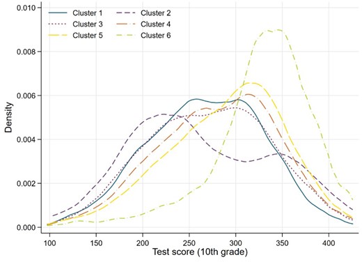
Kernel density of tests scores by cluster.
6.2 Main regression models
Table 4 presents our main estimates for the effect of studying in a given spatial cluster, with Cluster 3 being the reference category. We initially include four linear regression models based on Equation (3). Here, the dependent variable is the residual of a fixed effect regression with individual, school and year fixed effects. The SIMCE score in 10th grade is standardized, thus regression coefficients in the linear models are presented in standard deviations from the mean. In addition, we include two logit regressions: one for the probability of being in the bottom 40% of the distribution of standardized test scores, and one for the probability of being in the top 10% of the distribution. Estimates are presented as odd-ratios. We use the same dependent variable as in models 1–4 to construct our bottom 40% and top 10% binary variables (Table B6 in the Online Appendix presents the logit estimations including covariates one at a time).
Regression models for academic achievement in mathematics
| Residual SIMCE test score in 10th grade (OLS) | Logit bottom 40% | Logit top 10% | ||||
|---|---|---|---|---|---|---|
| Model 1 | Model 2 | Model 3 | Model 4 | Model 5 | Model 6 | |
| Cluster 1 | −0.024*** | −0.021*** | −0.021*** | −0.037*** | 1.156*** | 0.859** |
| (0.007) | (0.007) | (0.007) | (0.007) | (0.041) | (0.051) | |
| Cluster 2 | −0.016 | −0.024 | −0.032 | −0.040* | 1.096 | 0.610* |
| (0.026) | (0.025) | (0.025) | (0.022) | (0.151) | (0.159) | |
| Cluster 4 | 0.001 | −0.000 | 0.008 | 0.000 | 1.004 | 1.067 |
| (0.006) | (0.006) | (0.006) | (0.006) | (0.031) | (0.055) | |
| Cluster 5 | 0.005 | 0.002 | 0.015** | 0.040*** | 0.809*** | 1.217*** |
| (0.007) | (0.007) | (0.007) | (0.006) | (0.028) | (0.071) | |
| Cluster 6 | 0.057*** | 0.017* | 0.043*** | 0.067*** | 0.713*** | 1.283*** |
| (0.008) | (0.009) | (0.009) | (0.008) | (0.031) | (0.099) | |
| Female | −0.053*** | −0.054*** | −0.061*** | −0.007* | 1.056*** | 0.870*** |
| (0.004) | (0.004) | (0.004) | (0.004) | (0.021) | (0.029) | |
| Municipal public schools | −0.099*** | −0.139*** | −0.163*** | 1.965*** | 0.351*** | |
| (0.008) | (0.008) | (0.007) | (0.073) | (0.025) | ||
| Subsidized private school | −0.067*** | −0.104*** | −0.122*** | 1.649*** | 0.508*** | |
| (0.007) | (0.007) | (0.006) | (0.055) | (0.030) | ||
| Lagged test score (T-1) | −0.001*** | 0.002*** | 0.992*** | 1.003*** | ||
| (0.000) | (0.000) | (0.000) | (0.000) | |||
| Lagged test score (T-2) | −0.005*** | 1.023*** | 0.975*** | |||
| (0.000) | (0.000) | (0.000) | ||||
| Constant | 0.024*** | 0.092*** | 0.417*** | 1.170*** | 0.007*** | 85.578*** |
| (0.006) | (0.008) | (0.017) | (0.016) | (0.001) | (12.267) | |
| Observations | 50 265 | 50 265 | 50 265 | 50 265 | 50 265 | 50 265 |
| R-squared | 0.005 | 0.009 | 0.019 | 0.220 | ||
Robust standard errors clustered at the student level in parentheses. Reference category for type of school: private school. Reference category for clusters: Cluster 3. Models 1–4 use the residual from a previous fixed effect regression as dependent variable. OLS coefficients are measured in standard deviations of the SIMCE score. Logit coefficients are odd-ratios.
P < 0.01,
P < 0.05,
P < 0.1.
Models 1–4 incrementally include additional covariates. Model 1 only contains the spatial clusters and gender. Model 2 adds the type of school, that is, the difference in test scores due to attending a public school or subsidized private school as opposed to a fully private school. Model 3 incorporates the first lag, the test score of the same student in the 8th grade SIMCE test (in 2014), whereas Model 4 includes the second lag, the test score of the same student in the 4th grade SIMCE test (in 2010). As such, Models 3 and 4 address dynamic sources of bias through the inclusion of lagged values of the dependent variable.
Estimates for Models 1–4 are consistent. Relative to Cluster 3, both Cluster 1 and Cluster 6 report statistically significant effects. Exposure to the most marginalized districts (Cluster 1) negatively influences educational achievement (an effect of −0.04 to −0.02 standard deviations, depending on the included covariates), whereas exposure to the most privileged districts in the Metropolitan Region (especially Cluster 6) has a positive impact on test scores (an effect of 0.02–0.07 standard deviations). Exposure to areas with relatively poorer access to services (Cluster 2) has a similarly negative effect to exposure to Cluster 1 (−0.04 to −0.02 standard deviations). The effect of an upper-middle-class district (Cluster 5), on the other hand, is positive, albeit smaller than the effect of Cluster 6 (0.02–0.04 standard deviations). Finally, the effect of Cluster 4, a middle-class cluster with good access to services, is indistinguishable from that of Cluster 3. Overall, the effect of spatial context is driven by the extremes: exposure to either disadvantaged or advantaged areas has a significant effect on mathematics test scores. However, the size of these effects is not homogeneous. Relative to Cluster 3, the positive effect of exposure to privileged areas (Cluster 6) is around double the negative effect of exposure to the most marginalized areas (Cluster 1).
While these effects might appear small in terms of standard deviations, they are comparatively relevant and have substantial significance. Model 4 shows that the test score gap between Cluster 1 and Cluster 6 is of 0.104 standard deviations. This is almost two-thirds of the gap between private and public schools and equivalent to a gap of 50 points (a full standard deviation) in the previous SIMCE test. Given the fact that fully private schools represent two-thirds of all schools in Cluster 6 but only 2.1% of schools in Cluster 1 (see Table 3), our results suggest that school and spatial effects complement and reinforce each other, resulting in substantial gaps in test scores.
The logit regressions in Models 5 and 6 complement the previous estimates by analysing effects on top and bottom educational outcomes. Among those exposed to Cluster 1 and relative to Cluster 3, the odds of being in the bottom 40% of the test score distributions are 15.6% higher, while the odds of being in the top 10% are 14.1% lower. At the other end of the spatial distribution, among those exposed to Cluster 6, the odds of being at the bottom 40% are 28.7% lower and the odds of being at the top 10% are 28.3 higher, also relative to Cluster 3. Interestingly, the similarity in the size of the effects for each cluster suggests a homogenous treatment across the test score distribution. As such, Models 5 and 6 point to a polarizing effect: irrespective of individual characteristics and the type of school that adolescents attend, exposure to specific areas (particularly spatial divisions of poverty and wealth) pushes students towards one end of the distribution or the other.
Figure 3 summarizes our results. Panel A depicts the predicted standardized score (measured in standard deviations from the mean) for each cluster based on Model 4. Panel B shows the predicted probability of being in the bottom 40% of the test score distribution based on Model 5. Panel C illustrates the probability of being in the top 10% based on Model 6. Exposure to the most disadvantaged areas (Cluster 1) and those lacking access to services (Cluster 2) implies relatively lower educational performance, with the latter spatial cluster having a much larger confidence interval due to its small size. The areas in the middle (Clusters 3 and 4) report higher predicted outcomes than disadvantaged areas and present similar outcomes between them, consistent with the almost negligible coefficient for Cluster 4 reported in the models. Exposure to the most advantaged areas (Clusters 5 and 6) implies better educational achievement. Overall, and regardless of how we measure educational outcomes, the pattern is the same: exposure to more advantaged areas is strongly associated with higher test scores.1
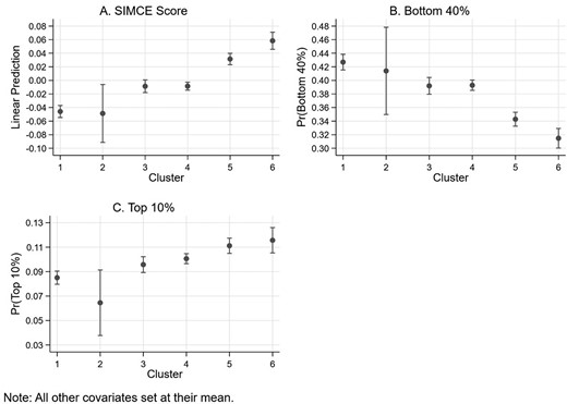
Adjusted predictions by spatial cluster with 95% CIs.
Closer analysis of Figure 3 reveals the differential spatial effects associated with more affluent and impoverished areas. The increase between the most disadvantaged areas (especially Cluster 1) and those in the middle (Clusters 3 and 4) is similar to that between Clusters 3 and 4 and upper-middle-class districts (Cluster 5). In other words, the negative effect of the most impoverished clusters is similar to the positive effect of the upper-middle-class cluster. However, all panels show an additional increment between Cluster 5 and the most privileged areas of the region (Cluster 6). This spatial cluster, which includes the four richest districts in Chile, shows a substantial increase in test scores that is clearly greater than the decrease suffered by the impoverished clusters.
In summary, we find that spatial context significantly affects educational achievement above and beyond the effect of individual and school characteristics. This is particularly true for the clusters representing spatial disadvantage and advantage. The former has a negative impact on educational achievement, whereas the impact of the latter is positive. As such, our results clearly support our first hypothesis. In addition, we find that the spatial effects on educational achievement appear stronger in affluent than marginalized areas, which also supports our second hypothesis. We provide several robustness checks to confirm our main findings in the Online Appendix (Section B).
7. Conclusions
We examined the effects of individual, school and spatial characteristics on the mathematics SIMCE scores of 10th grade students. Specifically, we analysed the effects of exposure to different areas of the Metropolitan Region of Santiago, Chile, the country’s most important and segregated urban agglomeration. Given the limited number of studies of affluent areas, we were particularly keen to explore how the advantages associated with these areas may enhance the educational achievement of adolescents and thus the socio-economic opportunities of the privileged. Instead of analysing separate spatial characteristics (i.e. poverty, density and access to facilities), we identified six major spatial clusters in order to represent spatial context, including concentrated poverty and wealth. We used different empirical strategies, which enabled us to account for bias from dynamic, time-invariant sources and provide several robustness checks. Our main conclusions are as follows.
First, our findings systematically showed that spatial context significantly affects educational achievement, above and beyond the effect of individual and school characteristics. In general, this result is in line with those reported in prior research focused on the influence of neighbourhood characteristics on educational outcomes (e.g. Owens, 2010; Otero et al., 2017; Wodtke and Parbst, 2017; Nieuwenhuis et al., 2019) and clearly supports the main expectation of the study. Specifically, we found that both concentrated advantage and disadvantage affect students’ mathematics test scores. Exposure to disadvantaged areas leads to lower student test scores, whereas exposure to advantaged areas leads to higher scores. Average effects are composed of the effects on high achievement and on low achievement. For instance, the positive impact of affluent areas is explained by both an increase in a student’s odds of being in the top 10% of SIMCE scores and a decrease in their odds of being in the bottom 40%. By contrast, the decrease in average scores in more disadvantaged areas marked by high levels of poverty, criminality and environmental hazards is explained by a strong increase in the likelihood of scoring in the bottom 40%. As such, our results point to a polarizing effect.
Second, we addressed a relevant issue in the literature concerning neighbourhood effects on educational outcomes: the potential role of concentrated advantage as opposed to the traditional emphasis on concentrated disadvantage or neighbourhood poverty (e.g. Johnson, 2013; Howell, 2019). In this regard, we find evidence to support our second hypothesis, that spatial effects on educational achievement would appear stronger in advantaged than disadvantaged areas. Indeed, our results showed that the positive effect of affluent areas is greater than the negative effect of impoverished areas. These differential effects relating to spatial context constitute a relevant issue to which the present paper has contributed. Their existence holds powerful implications for both the literature on neighbourhood effects and policies aimed at reducing spatial inequality (e.g. Galster, 2018). In brief, our results suggest that the problem concerns not only the concentration of poverty, but also the growing trend of concentration of affluence in cities. Residential advantage seems to be particularly relevant for the reinforcement of educational inequality and upper-class reproduction.
Third, it is important to bear in mind that the approach taken in the present study for clustering districts does not enable us to discern the specific way in which various components and thus specific mechanisms separately contribute to the observed variation in student achievement. Rather, our approach allows us to focus on the intersectionalities between different spatial attributes. On the one hand, we demonstrated that residential disadvantage goes hand in hand with low educational level, experiences of violence (e.g. fights and shootings), trash on the streets, pest infestations and drug availability. This may suggest that the effect of disadvantaged areas on negative educational achievement is probably driven by a combination of socialization and institutional mechanisms (e.g. Harding, 2011; Sharkey and Faber, 2014). On the other hand, we showed that concentrated wealth goes hand in hand with high levels of education, access to services and network availability. As such, the positive effect of affluent areas on academic achievement may be channelled not only by a planned, intentional and homogeneous parenting style among affluent residents (Lareau, 2011; Lareau and Goyette, 2014), but also by the existence of residential cohesion. In this regard, social organization and social ties may be operating as tools that the residents of affluent neighbourhoods use as an essential part of their privilege (e.g. Méndez and Gayo, 2019; Méndez et al., 2020). In short, this is an indication that both residential advantage and disadvantage are the result of a combination of specific components that work together, and that the likelihood that some mechanisms act alone to positively or negatively affect educational outcomes is limited. As such, although attempts to separate neighbourhood effects are laudable, they might be somewhat detached from the ‘true’ functioning of the spatial structure.
The present study has some weaknesses that merit acknowledgment. First, although we used a wide range of variables to represent spatial context, we were unable to determine how changes in segregation patterns over time have generated variations in student performance. To do so would require a dynamic characterization of the spatial structure based on spatial indicators for different moments in time. Second, we were unable to establish the degree to which neighbourhood effects on educational achievement vary according to timing (differential effects of early versus late exposure) and duration of exposure (short spells of exposure versus prolonged exposure to surrounding conditions) (e.g. Wodtke et al., 2011; Musterd et al., 2012). To solve these problems, researchers could collect data concerning the time of students’ exposure to residential environments and study the neighbourhood effects at different points in the students’ lives (e.g. Nieuwenhuis et al., 2019). Third, the structure of our data—in particular the fact that most students do not change clusters over time—does not allow us to directly estimate a fixed effect regression model, which is why we proposed a two-step correction to address time-invariant sources of bias.
Finally, we were not able to compare our results at the district level with the effects associated with smaller geographical scales (e.g. census areas and blocks). It is likely that the effects of spatial context are only visible on a larger scale where the gap between rich and poor is generally more apparent. Regarding this, it is also probable that the mechanisms that channel neighbourhood effects become more or less important depending on the spatial scale in question (e.g. Sharkey and Faber, 2014). For example, socialization mechanisms probably operate on smaller scales, while institutional mechanisms are more relevant on wider geographical scales, as they respond to more structural aspects of the urban geography (see also Otero et al., 2017). Researchers could attempt to solve this issue by tackling the following questions: At which spatial scale do we observe larger spatial effects on academic performance? Which spatial mechanisms are the main contributing factors to educational inequality at smaller scales? These are relevant challenges for future research which, if tackled, could improve our understanding of spatial divisions and their effects on various outcomes.
Footnotes
We did not find major differences when re-estimating our models for a men-only or women-only sample, suggesting that gender differences are not statistically significant. While we do not report these findings, they are available by request.
Acknowledgements
The authors are grateful for support from the Centre for Social Conflict and Cohesion Studies—COES. Comments from three anonymous referees have led to substantial improvements in the paper.
Funding
The authors disclosed receipt of the following financial support for the research, authorship and/or publication of this article. This work was supported by the National Agency of Research and Development (ANID) at the Chilean Ministry of Science, Technology, Knowledge and Innovation, grant/award numbers: ANID/FONDAP/15130009; ANID PFCHA/DOCTORADO BECAS CHILE/2017—72180515 and ANID PFCHA/DOCTORADO BECAS CHILE/2016—72170193. This work was also supported by ANID through its Millennium Science Initiative Program, grant/award number: NCS17—015.
Supplementary material
Supplementary material is available at SOCECO Journal online.
Declaration of conflicting interests
The author(s) declared no potential conflicts of interest with respect to the research, authorship and/or publication of this article.
