


Abstract
The Great Recession raised the concern that employment protective institutions that are effective during macroeconomic stability might become counterproductive under growing macroeconomic volatility. We study this question by examining the relationship between employment protection legislation (EPL) and unemployment scars on earnings in 21 countries during the period surrounding the Great Recession. We use harmonized work history data for 21 countries from 2004 to 2014 and combine propensity score matching and multilevel-regression to estimate how earnings losses due to unemployment vary with the strength of labor market regulation and over changing macroeconomic conditions. We find that unemployment scarring is lower in contexts with robust employment protection, both under positive and negative macroeconomic environments. We also show that economic downturns intensify unemployment scarring significantly more in countries with weak EPL, largely because long-term unemployment is more strongly penalized. Taken together, our study finds that the positive effects of employment protection for workers remain robust during economic downturns.
1. Introduction
The dramatic rise in unemployment during the Great Recession reinvigorated the debate about employment protection legislation (EPL; i.e. Palier and Thelen, 2010; European Commission, 2011; Countouris and Freedland, 2013; Muffels et al., 2014). EPL sets standards for how workers can be fired and hired, by mandating severance payments, advanced notice of dismissal or setting limits on contracts through temporary work agencies. EPL ranges in a continuum from low to high (or weak to strong), depending on the required costs and procedures involved in hiring and dismissing workers. Supporters of a strong EPL say that these regulations can successfully generate good quality jobs and shelter workers from severe economic uncertainty without undermining macroeconomic performance (Backer et al., 2005; Gangl, 2006; Baccaro and Rei, 2007; Bauer et al., 2007; Howell et al., 2007; Howell and Rehm, 2009; Vergeer and Kleinknecht, 2012; Countouris and Freedland, 2013; Hastings and Heyes, 2018). Critics say that strong EPL blocks firms’ flexibility and capacity to adapt to changing economic environments, slowing economic growth and innovation (European Commission, 2002, 2007, 2011, 2012; IMF, 2003; Bauer et al., 2007; Bierhanzl, 2008; Kugler and Pica, 2008; Bernal-Verdugo et al., 2012; OECD, 2013). Critiques of EPL have been around for a long time (Palier and Thelen, 2010), but have become more prominent in the context of the Great Recession with the premise that EPL might no longer be effective in a globalized and highly volatile macroeconomic environment (Countouris and Freedland, 2013; Muffels et al., 2014; Hastings and Heyes, 2018). The current wave of criticism stresses that while EPL might have had positive equilibrium effects in previous industrial economies, the rigidities of these policies are increasingly disadvantageous in a context where constant flexibility and innovation is necessary, particularly during economic downturns (European Commission, 2012; Muffels et al., 2014; Hastings and Heyes, 2018).
Our article intervenes in this debate by studying whether EPL accentuates the negative consequences of economic recessions for workers who lose their jobs. Building on previous literature on unemployment scarring on earnings (Farber, 2005; Gangl, 2006), we examine how the degree of EPL and variation in macroeconomic environments shape workers’ post-unemployment earnings losses in the period surrounding the Great Recession. Unemployment scarring on earnings is a useful summary measure that captures how job losses affect the likelihood of re-employment, re-unemployment, post-unemployment job match and quality, and workers’ overall exposure to economic uncertainty and volatility (Farber, 2005). If critics are right, EPL will amplify the negative consequences of economic recessions on labor market conditions and worsen unemployment scarring on workers’ earnings. In other words, earnings penalties to unemployment will increase during a recession more in a context with higher EPL. If EPL supporters are instead right, economic recessions will not worsen unemployment scarring more in contexts with stronger EPL in place.
Previous research on unemployment scarring on earnings examined variation across labor policy regimes and macroeconomic environments separately. Studies concerning labor policy regimes have largely focused on periods of economic stability or growth. These studies find that higher EPL is associated with longer unemployment duration (Gangl, 2004a, 2004b) but smaller earnings scarring (Gangl, 2006). Research on unemployment scarring across macroeconomic environments, on the contrary, has been largely based on single-country studies and has not paid attention to labor market institutions such as EPL. Earlier studies in the USA found that economic recessions do not substantially worsen earnings scarring (Farber, 1997, 2005), but more recent studies find that economic recessions do worsen earnings scarring, showing that workers who lose jobs during a recession experience longer unemployment spells and greater earnings losses (Gangl, 2006; Couch et al., 2010; Couch et al., 2011). Neither of these bodies of research has considered the interaction between labor market institutions and macroeconomic environment, thus leaving open the possibility that high EPL’s seemingly virtuous outcome to reduce unemployment earnings scarring might wash away in a context of growing macroeconomic volatility.
The interaction between EPL and macroeconomic shocks has been examined in an adjacent literature that focuses on aggregate-level unemployment rates, rather than unemployment scarring. Blanchard and Wolfers (2000) proposed the institution-shock framework to argue that the impact of shocks on unemployment rates varies across institutional environments. They used this model to explain changing disparities in unemployment rates between the USA and European countries. This body of research finds that shocks increased unemployment rates more in contexts with strong EPL compared to other contexts (Blanchard and Wolfers, 2000; Bertola et al., 2001; Blanchard and Portugal, 2001; Autor et al., 2007). More recent research, however, has disputed these findings and showed that they are very sensitive to model specification (Avdagic and Salardi, 2013). Related studies on labor market flows, which examine mobility rates and typical length of employment and unemployment, also considered the interaction between labor market institutions and macroeconomic environment, finding that market flows are generally lower in contexts with high EPL and less sensitive to macroeconomic shocks (DiPrete et al., 1997; DiPrete and Nonnemaker, 1997). While informative, the findings from this literature are inconclusive about how the interaction between EPL and macroeconomic environment can affect unemployment scarring on earnings. For instance, high EPL could worsen unemployment scarring through increased long-term unemployment, even if it does not lead to greater increases in the unemployment rate. Alternatively, high EPL might continue to protect workers from experiencing elevated earnings losses despite market flows being less responsive to macroeconomic shocks.
In this article, we examine four possible pathways through which the interaction between EPL and macroeconomic environment can shape unemployment scarring on earnings: employer reluctance to hire, unemployment stigma, labor market segmentation and wage dispersion. We employ harmonized individual-level work history data built from panel survey datasets covering 21 European and North American countries for the years 2004–2014 and we merge it with country-specific time-varying measures of EPL, macroeconomic environment, and other relevant context-level labor market institutions. Our analyses use difference-in-difference (DiD) propensity score matching to estimate unemployment earnings scarring, comparing earnings change between workers who experience job loss with earnings change among similar workers who do not experience job loss. We use multi-level linear regression models to estimate how context-level EPL and macroeconomic environment shape the magnitude of unemployment earnings scarring. Our article makes three contributions to the existing literature. First, we offer an empirical test for the hypothesis that EPL’s effectiveness at protecting workers might be contingent on positive macroeconomic environments. Second, we update existing research on earnings scarring across welfare regimes and across macroeconomic environments with new data and assess whether previous conclusions hold up. Third, we expand the number of countries covered in the analysis thus increasing variation in both institutional characteristics and macroeconomic environment.
The results show that EPL is effective at reducing unemployment earnings scarring even under negative macroeconomic conditions. Workers who lose jobs in countries with higher EPL experience smaller earnings losses than their counterparts in countries with weaker EPL, both in periods of economic growth and during economic downturns. Workers in countries with weaker EPL experience large increases in earnings scarring as macroeconomic conditions deteriorate. This pattern is neither due to differences or differential change in unemployment duration or in the composition of the unemployed workforce, nor it is due to the interaction with other labor market institutions, such as unemployment benefit generosity. Instead, we find this pattern to be driven by substantially higher earnings penalties associated with long-term unemployment in contexts with weaker EPL. Economic recessions increase long-term unemployment across the board, but loss of earnings due to long-term unemployment is much higher in low-EPL contexts than in high-EPL contexts. Thus, contrary to critics of EPL, we find robust evidence that stronger EPL continues to protect workers from severe unemployment earnings scarring even in a context of growing macroeconomic volatility.
2. Background
The literature on economic unemployment scarring shows that losing a job is associated with long-lasting declines in earnings, work quality and often with unemployment reincidence (Ruhm, 1991; Farber, 1993; Gangl, 2004a; Brand, 2015, 2006). Research on unemployment scarring on earnings shows that earnings losses are higher when workers take longer to find a job, when they switch jobs or occupational categories, and when workers are highly skilled or have tenure (Carrington and Zaman, 1994; DiPrete and Nonnemaker, 1997; Stevens, 1997; Kletzer, 1998; Farber, 2005). Studies show that both labor market institutions and macroeconomic environments can substantially accentuate or reduce unemployment scarring on earnings.
Research on labor market institutions has largely focused on unemployment insurance (UI) and EPL. Several studies find that both policies are associated with longer unemployment spells (OECD, 2004, 2006; Lalive, 2007; Kugler and Pica, 2008), suggesting that this translates into greater unemployment scarring on earnings as well. But other studies find that both UI benefits and EPL are associated with higher employment stability after job loss (Wulfgramm and Fervers, 2015), better job matches (Gangl, 2004b) and smaller earnings scarring (DiPrete and McManus, 2000; Gangl, 2006). Recent studies challenge some of these findings for EPL, showing that higher EPL is associated with stronger barriers to enter high-quality jobs after unemployment (Dieckhoff, 2011), particularly for marginalized workers (Kahn, 2007).
Research focused on the macroeconomic environment shows that unemployment scarring on earnings varies across these contexts too. Recent studies estimate that long-term earnings losses increase between 2% and 4% when job losses occur in a context of economic recession (Couch et al., 2010; Couch et al., 2011; Davis and Von Wachter, 2011). This recent set of studies contradicts previous research that had found no substantial differences in unemployment earnings scarring across periods of economic growth and recession (Farber, 1993, 1997, 2005). It is still unclear if this discrepancy in results is indicative of a change in labor market dynamics or due to differences in identification and estimation approaches.
Both sets of literatures on labor market institutions and on macroeconomic environments show that unemployment scarring on earnings is shaped by the types of jobs that are lost, the typical length of unemployment, and the conditions of the jobs unemployed workers eventually find. On average, unemployment scarring is greatest when it affects workers with the best jobs and workers get much lower quality jobs after unemployment. Scarring is the smallest when it is more likely to affect workers with lower quality jobs and workers can easily go back to similar jobs afterward. Building on existing research, we describe four context-based processes that can shelter workers or make them more susceptible to unemployment scarring: employer reluctance to hire, unemployment stigma, labor market segmentation and earnings dispersion.
2.1 Employer reluctance to hire
Standard economic theory argues that constraints on and costs of layoffs (i.e. high EPL) turn employers into conservative hirers and reduce economic dynamism (OECD, 1999, 2004). When employers cannot fire workers at will, every hiring decision becomes potentially costly, and employers only hire when they absolutely need to. This line of argument is consistent with research finding that market flows are lower in contexts with stronger EPL (Bertola and Rogerson, 1997; DiPrete et al., 1997, 2001; Bertola, 1999; Layte et al., 2004), although some recent studies challenge these findings (Bauer et al., 2007; Kugler and Pica, 2008). This argument is also consistent with studies finding that unemployed workers take longer to find a job in a context with stronger EPL (Machin and Manning, 1999; Bernardi et al., 2000; Behaghel et al., 2008; Skedinger, 2010). As longer periods of unemployment aggravate loss of human capital and deteriorate job search networks, they are expected to result in higher unemployment scarring on earnings too.
Because economic recessions increase economic uncertainty, they are also likely to increase employer reluctance to hire, regardless of the institutional environment. Studies show that increases in long-term unemployment were widespread and long-lasting during the Great Recession (Kroft et al., 2016), indicating that employers hesitated to open new positions. However, it is unclear if employers in different institutional environments would react similarly to a shock in economic uncertainty. This perspective raises the possibility that a negative macroeconomic environment might further exacerbate employer reluctance to hire in contexts with higher EPL, producing an echo effect that stalls economic dynamism and worsens long-term unemployment and its associated earnings penalties. It is also possible, however, that when employer reluctance to hire is already high, the added effect of macroeconomic uncertainty might be smaller or not substantially different from its effect in other contexts.
2.2 Unemployment stigma
Signal theory argues that scarring occurs because employers rely on signals to choose their workers and unemployment is seen by employers as a negative sign about workers’ productivity. In their seminal work, Gibbons and Katz (1991) showed that workers who lost jobs in mass layoffs had smaller earnings scarring than those who lost jobs due to regular dismissals, arguing that only in the latter case was unemployment used as a sign about workers’ quality. This theory also poses that the higher the uncertainty and costs to hiring decisions, the more likely employers are to use signals and thus to discriminate against unemployed workers. Indeed, several studies have found evidence in this direction (Canziani and Petrongolo, 2001; Kugler and Saint‐Paul, 2004; Gangl, 2004b; Holden and Rosén, 2014). For instance, Gangl (2004b) finds that workers with long unemployment spells are penalized more severely in protected jobs both in the USA and Germany, and Kugler and Saint-Paul (2004) find that US states with higher firing costs are associated with lower re-employment probabilities for unemployed workers. A recent study challenges this hypothesis showing that workers who were laid off are not more likely to get temporary contracts than those who lost jobs in plant closures (Biegert and Kühhirt, 2018). This perspective suggests that unemployment stigma is worse in contexts with higher EPL due to the higher costs of hiring decisions, but it is unclear how macroeconomic uncertainty might interact with unemployment stigma. Macroeconomic uncertainty could exacerbate unemployment stigma in contexts with higher EPL but, because the levels of stigma might be already relatively higher in those contexts, it is very plausible that unemployment stigma is more cyclical in contexts with lower EPL. Employers in contexts with lower EPL have fewer constraints on setting wages and more discretion in evaluating worker’s characteristics (including unemployment history), which may come into play more strongly in a context of high macroeconomic uncertainty and increase unemployment scarring on earnings.
A different approach on unemployment stigma links its prevalence to social and cultural norms. Researchers show that labor institutions shape the extent to which unemployment is perceived and experienced as the individual’s fault (Newman, 2013; Sharone, 2013). Sharone (2013), for instance, argues that prevailing cultural norms make US workers more likely to blame themselves for job losses than Israeli workers. Further, political economy scholars suggest that EPL is tied to cultural commitments to full-time employment that accentuate structural rather than individual blame for unemployment (Tahlin, 2013). This argument suggests that unemployed workers might be less severely discriminated against in contexts where unemployment is less likely to be seen as the fault of an individual and that in such contexts unemployed workers, even if long-term unemployed, might be less likely to accumulate negative effects of employer discrimination.
2.3 Labor market segmentation
The labor market segmentation approach emphasizes how labor market structure shapes which workers are most likely to lose jobs. Scholars argue that labor market segmentation reduces overall unemployment scarring on earnings by concentrating on unemployment risks among the contingent and often low-skilled workforce (Esping-Andersen, 2000; Kletzer and Fairlie, 2003; Gangl, 2006). Low-wage workers who lose a job are more likely to find a job that pays more or less the same as their previous job and experience generally low unemployment scarring on earnings. At the same time, labor market segmentation protects workers with good jobs through provisions that make their dismissal costlier, and through sectoral boundaries that protect benefits and returns to skills provided that unemployed workers can manage to remain in the same sector after unemployment (Sorensen, 2000; Estevez-Abe et al., 2001; Weeden, 2002). Because higher EPL is tightly connected to segmented labor markets (Biegert, 2017), several scholars argue that this compositional effect is what maintains low unemployment scarring on earnings in these contexts (Gangl, 2006).
This approach raises the possibility that economic shocks could weaken the protection that ‘insider’ workers enjoy as companies are forced to restructure, resulting in higher unemployment scarring on earnings. An economic downturn could also lead to more workers crossing sectoral and occupational boundaries even though the penalties to this form of mobility are typically greater in segmented labor markets, thus increasing earnings scarring (Bertola and Rogerson, 1997; Cha and Morgan, 2010). This set of processes seems plausible particularly during recessions that involve major economic restructuring and displace entire sectors of the economy, e.g. construction sector in the USA, Spain, and Estonia during the Great Recession (Tahlin, 2013). This pattern suggests that economic recessions might worsen unemployment scarring on earnings more in a context with stronger EPL than in contexts with weaker EPL.
An alternative expectation would indicate that ‘insider’ workers might remain protected even during mass layoffs in economic downturns. In fact, ‘insider’ workers might be more protected during a recession than equivalent high-wage and high-tenure workers in contexts with weak employment protection. This is consistent with research showing that highly skilled workers are more protected from unemployment risks in countries with higher EPL, at least during contexts of economic growth (DiPrete et al., 1997; DiPrete and McManus, 2000).
2.4 Earnings dispersion
Unemployment scarring on earnings is partly a function of wage inequality in the labor market, with greater disparity increasing the potential for elevated scarring on earnings. Scholars argue that EPL is often connected to reduced wage dispersion and higher wage floors through diffuse institutional mechanisms related to other labor market legislation, such as minimum wage or unionization (Gangl, 2006; Biegert, 2017). Previous studies suggest that wage dispersion is one potential explanation for the smaller unemployment scarring on earnings in contexts with higher EPL (Gangl, 2006).
Researchers suggest that EPL mechanisms can limit the extent to which companies can resort to lowering wages to adjust to negative macroeconomic conditions (Machin and Manning, 1999; Bernardi et al., 2000; Behaghel et al., 2008; Skedinger, 2010). This reasoning implies that economic downturns might exacerbate earnings dispersion more in contexts with weaker employment protections and potentially accentuate unemployment scarring on earnings as a result. On the contrary, studies have shown that wage inequality grew substantially during the recent Great Recession in contexts with robust EPL too (Grusky et al., 2011). This suggests that the protective effect of compressed wage dispersion associated with higher EPL might disappear in a context of economic volatility and no longer protect workers from severe earnings losses.
2.5 Hypotheses
The previous discussion summarizes four sets of processes that can shape unemployment scarring on earnings. These four types of mechanisms are linked to different theoretical traditions (the reluctance to hire and the uncertainty-related unemployment stigma processes are common in mainstream economic, and the labor segmentation, inequality, and culture-related unemployment stigma are common in institutional economics or sociology), but they are not mutually exclusive and several mechanisms could be empirically operating at the same time. Our discussion has centered on describing the implication of each of these mechanisms for the relationship between unemployment scarring on earnings and EPL, macroeconomic conditions, and the interaction between the two.
This discussion presents various processes whereby negative macroeconomic conditions could be expected to increase unemployment scarring more in contexts with lower EPL than in contexts with higher EPL, as well as various processes whereby the negative macroeconomic conditions could be expected to increase unemployment scarring more in contexts with higher EPL than contexts with lower EPL. We summarize these expectations in two hypotheses:
H1: Economic recession will worsen unemployment scarring on earnings more in contexts with high EPL. This outcome could result because:
EPL’s higher costs to hiring and firing will accentuate employer reluctance to hire and result in longer unemployment spells and higher earnings losses.
EPL’s higher costs to hiring and firing will accentuate unemployment stigma and result in longer unemployment spells and higher earnings losses.
Increased layoffs of ‘insider’ workers and/or increased mobility across sectors and industries in segmented labor markets contexts with high EPL will increase the prevalence of large earnings losses.
Increased earnings dispersion in contexts with robust EPL will increase the prevalence of large earnings losses.
H2: Economic recession will worsen unemployment scarring on earnings more in contexts with weak EPL. This outcome could result because:
Employer reluctance to hire will increase more in lower EPL contexts than in higher EPL contexts where this reluctance is already high.
EPL is associated with stronger barriers to employers’ ability discriminate based on workers’ (un)employment history as well as with cultural values that lower unemployment stigma and mitigate large penalties associated with long-term unemployment.
EPL continues to protect ‘insider’ workers in segmented labor markets while high-skilled and high-paid workers in weak EPL contexts face increased risks of losing their job, thus increasing the prevalence of large earnings losses.
Increased earnings dispersion in contexts with weak EPL will increase the likelihood of large earnings losses.
3. Data, measures and methods
3.1 Data
We use panel data for workers’ employment and earnings history in 21 countries for the years 2004–2014. We harmonized five major panel surveys: the US Survey of Income and Program Participation (SIPP), the European Union Statistics on Income and Living Conditions (EU-SILC), the German Socioeconomic Panel (GSOEP), the British Household Panel Study (BHPS) and the Understanding Societies Survey (UKHLS). All these are household surveys containing the most high-quality longitudinal information on work and employment in the USA and Europe. Because there are some differences in survey design, we harmonized all datasets to reflect the EU-SILC design that offers the maximum common denominator. The EU-SILC has a 4-year rotating panel structure and conducts interviews once per year. Respondents report monthly employment information and annual earnings from the year prior to the interview. The Online Appendix includes more detailed information about the harmonization steps.
Our sample is comprised of 130,414 workers 16–60 years of age and employed at the time of the first interview and report positive earnings for the year before the first interview. This means that, like other studies (Farber, 2005; Gangl, 2006), our sample represents adults who are already attached to the labor market. Our treatment group is made up of workers who lose jobs between the second and third interview and our control group is made up of workers who remain employed in that period. This identification choice allows us to have a treatment group for whom we observe earnings around 2 years prior to job loss and earnings from jobs after unemployment. Based on prior research finding that unemployed workers’ earnings start declining right before job loss (Ruhm, 1991; Stevens, 1997), we want to match the treated and control groups on worker and job characteristics over a year before job loss. See the Online Appendix for more information about the construction of the analytic sample.
3.2 Measures
Job losses are transitions from employment to unemployment. We identify these shifts in employment status using respondents’ monthly records on economic activity. Employment status is defined as having a job even if not currently at work, this definition makes sure that workers on holidays or on leave are classified as employed. A job loss is identified when respondents move from having a job to not having a job, which could be due to layoffs, end of contract or quitting a job, our data cannot distinguish between these various forms of job loss. Our measure includes job losses that result in at least 1 month of unemployment and it includes unemployment spells of varying duration. This means that our treated group includes workers who lose jobs and regain employment anytime between 1 month after the job loss to more than 1 year after the job loss.
Monthly earnings are estimated using the worker’s annual earnings reports divided by the number of months in employment in that year. Earnings are harmonized to 2005 EUR. All earnings measures are logged, thus a change in this earnings measure can be interpreted as percentage change. Ideally, we would prefer to calculate hourly wages, but the EU-SILC does not include information on usual work hours corresponding to the income reference period. Our measure is also imperfect because it does not allow for a perfect fit between jobs and wages, e.g. a worker who switches jobs during the year will be given the value of the average wage instead of the wage corresponding to each job. While better information is available in some panel surveys (SIPP, GSOEP, BHPS), detailed information is not available in the EU-SILC. We adjusted the analytic design to this feature of the data so that it does not pose a problem for our analyses. The unit of analysis in our study is the year and our measures of pre- and post-unemployment wages are taken from separate calendar years before and after unemployment. This guarantees that our wage measure does not average over pre- and post-unemployment jobs. See the Online Appendix section ‘Analytic Sample’ for more details on the construction of this variable.
Employment protective legislation (EPL) is a country-level time-varying measure that captures the rigidity of employment regulations. We use the OECD synthetic index of strictness of employment protection in individual and collective dismissals. The index compiles information on three main dimensions: procedures and costs involved in individual dismissal of workers on regular contracts, additional costs for collective dismissals and regulation of temporary contracts.1 In our sample, this index ranges from 0.25 to 3.21, with higher values indicating stronger employment protection. For instance, a country with high penalties for firing senior workers will score higher than a country with low penalties for firing senior worker, all else being equal. It is important to note that measuring EPL in a single index necessarily simplifies the existing policies and does not capture all variations and dimensions of this body of social policy. This measure, for instance, does not distinguish between temporary and permanent workers. Notwithstanding these caveats, the measure we use is the best harmonized synthetic measure to compare countries in the relative strength of employment protection.
Unemployment rate change (UR) is the country-level time-varying measure that we use to capture the macroeconomic environment,2 with growing levels of unemployment indicating a negative macroeconomic environment and declining levels of unemployment indicating an improving and positive macroeconomic environment. We use Eurostat statistics on year-to-year changes in the annual average unemployment at the country level. The main substantive reason to use the unemployment rate as a macroeconomic indicator is to measure directly the state of the labor market, so that our estimates compare workers in different institutional contexts but similar labor market conditions. Additionally, using changes in the unemployment rate as our key indicator means that our estimates set aside the macro-level relationship between EPL, economic recession and unemployment rate explored in adjacent literatures (i.e. Blanchard and Wolfers, 2000; Avdagic and Salardi, 2013).
3.2.1 Other individual-level variables
Our models include standard control variables for workers’ human capital, occupation and job characteristics. Age is coded as a continuous variable. Education level is summarized in three categories (1 = high school or less; 2 = post-secondary no college degree; 3 = college degree and above). Work hours are coded as a continuous variable, ranging from 1 to 80 hours per week. Job tenure is a dummy variable that indicates whether the worker had the job for over a year. Occupation specific characteristics are measured using dummy variables for each of the ISCO-08 single-digit occupations.
3.2.2 Other country-level control variables
Our models also include controls for country-level characteristics that could confound the relationships of interest. Drawing on previous research on the institutional policies that correlate with EPL and with the consequences of job loss (Gangl, 2006; Biegert, 2017), we include measures for unemployment insurance benefits (UI) and union density (UD). We use OECD data to construct both measures. Including a measure of UI benefits is crucial because previous research has shown it can prolong the duration of job search (Gangl, 2004a, 2004b) and it is a common policy instrument in contexts that also have higher EPL. Failing to control for UI benefit generosity could lead our employment protection measure to pick up this correlation and over-estimate its correlation with unemployment duration and earnings scarring. A similar logic motivates the inclusion of UD. Higher UD correlates with EPL and is related to labor market processes that can result in lower unemployment scarring, such as collective wage agreements that constrain employers’ ability to make wage offers dependent on previous (un)employment history.
Separating the independent effects of different labor market institutions is challenging because certain combinations of policies are more common than others and because policies have different effects in different contexts (Hall and Soskice, 2004; Hall and Thelen, 2008). A reasonable estimation requires, for instance, sufficient variation in unemployment benefits across contexts that have similar levels of EPL. Table 1 provides a summary of all key macro-level variables. The country with the highest EPL score is the Czech Republic at 3.21, while the USA has the lowest score at 0.26. The average change in unemployment rates is positive, denoting general increases in unemployment rates across this period. Variation in UI generosity ranges from a high of 6.47 in Denmark to a low of 1.13 in Poland, whereas variation in UD ranges from a high of 73% in Sweden to a low of 8% in France. Figure 1 illustrates the changes in the unemployment rate for our sample of countries between 2003 and 2014. This figure shows that although the vast majority of countries experienced substantial increases in the unemployment rate during the Great Recession, countries were not all hit equally hard nor exactly at the same time or for the same length of time. It is due to this pattern of heterogeneity that it is particularly appropriate to use country-specific time-varying measures to identify levels of labor market stress (in our case the unemployment rate) instead of relying on cruder measures such as pre-/post-recession dummies.

Changes in annual unemployment rate around the great recession.
Notes: Changes in annual unemployment rate measure year-to-year differences in annual unemployment rate. For instance, a value of 1 indicates that the unemployment rate in that year is 1 percentage point higher than in the previous year.
Source: OECD Statistics
Descriptive statistics for key macro-level variables
| (1) | (2) | (3) | (4) | |||||
|---|---|---|---|---|---|---|---|---|
| UR | EPL | UI | UD | |||||
| Unemployment Rate (annual change) | EPL | Unemployment Insurance Generosity | Union Density | |||||
| Mean | SD | Mean | SD | Mean | SD | Mean | SD | |
| POOLED | 0.04 | 1.56 | 2.05 | 0.90 | 2.74 | 1.39 | 25.03 | 16.01 |
| AT | −0.08 | 0.60 | 2.37 | 0.00 | 4.87 | 0.36 | 30.21 | 2.04 |
| BE | −0.16 | 0.66 | 1.92 | 0.07 | 3.34 | 0.12 | 54.34 | 0.47 |
| CZ | −0.54 | 1.05 | 3.21 | 0.12 | 2.85 | 0.12 | 18.88 | 1.53 |
| DE | −0.72 | 0.56 | 2.68 | 0.00 | 4.38 | 0.26 | 19.82 | 1.47 |
| DK | 0.49 | 1.23 | 2.13 | 0.00 | 6.47 | 0.32 | 68.57 | 1.51 |
| EE | 0.52 | 3.92 | 2.62 | 0.32 | 1.52 | 0.07 | 8.53 | 1.09 |
| EL | 1.69 | 2.58 | 2.80 | 0.00 | 1.19 | 0.14 | 23.87 | 0.25 |
| ES | 2.47 | 2.23 | 2.36 | 0.00 | 3.63 | 0.05 | 16.13 | 1.26 |
| FI | −0.14 | 0.78 | 2.17 | 0.00 | 4.97 | 0.22 | 69.86 | 0.93 |
| FR | 0.27 | 0.62 | 2.42 | 0.04 | 4.44 | 0.23 | 7.68 | 0.07 |
| HU | 0.48 | 0.76 | 2.00 | 0.00 | 2.75 | 0.24 | 15.65 | 1.35 |
| IE | 0.10 | 0.08 | 1.38 | 0.08 | 3.36 | 0.41 | 34.05 | 0.82 |
| IT | 0.34 | 1.01 | 2.76 | 0.00 | 3.53 | 0.10 | 34.25 | 0.79 |
| LU | 0.03 | 0.35 | 2.25 | 0.00 | 3.59 | 0.10 | 36.26 | 1.58 |
| NL | 0.06 | 0.66 | 2.86 | 0.03 | 3.91 | 0.30 | 19.85 | 0.82 |
| PL | −1.18 | 2.26 | 2.23 | 0.00 | 1.13 | 0.09 | 16.29 | 1.56 |
| SE | 0.11 | 1.04 | 2.61 | 0.00 | 2.41 | 0.20 | 73.99 | 2.93 |
| SI | 0.49 | 0.94 | 2.65 | 0.00 | 3.04 | 0.17 | 30.10 | 5.07 |
| SK | −0.87 | 1.93 | 2.22 | 0.00 | 1.37 | 0.01 | 20.16 | 2.69 |
| UK | 0.10 | 0.31 | 1.26 | 0.00 | 1.58 | 0.03 | 27.19 | 0.30 |
| USA | 0.05 | 0.38 | 0.26 | 0.00 | 1.19 | 0.02 | 11.93 | 0.05 |
Notes: (1) UR uses Eurostat statistics on annual changes in the aggregate country-level unemployment rate, the mean reports the average annual change in the unemployment rate between 2003 and 2014 in each country; (2) EPL uses OECD Statistics on strictness of employment protection individual and collective dismissals; (3) UI is an index computed using OECD Statistics data on UI coverage (UCOV) and spending on unemployment benefits (UBEN) and on a subset of active labor market policies that focus on income protection (ALMPT), the index is calculated as follows UCOV × (UBEN + ALMPT) × 10/2; (4) UD uses UvA ICTWSS database on UD calculated as the net union membership as a proportion of wage and salary earners in employment.
Sources: OECD Statistics, Eurostat Statistics and UvA ICTWSS database.
3.3 Methods and analysis plan
We combine DiD propensity score matching with multi-level regression to model how institutions and macroeconomic conditions shape the consequences of job loss. Our analysis involves three steps: (a) balancing our treated and control sample with propensity score matching to estimate DiD within-person changes in monthly earnings associated with job loss (this is our measure of unemployment scarring on earnings), (b) modeling the relationship between unemployment scarring on earnings across EPL and macroeconomic environments, and (c) examining the mechanisms that drive this relationship.
The goal of the first step is to obtain an estimate about the amount of monthly earnings workers lose as a result of job loss. Following common practice in this literature (i.e. Gangl, 2006), we use propensity score matching to balance the distributions of treatment and control groups to obtain a causal estimate of the consequences of job loss. Given that we base the analysis on panel data, we are able to employ a DiD matching estimator that conditions the analysis on all (observed or unobserved) stable characteristics of individual respondents (see Heckman et al., 1997, 1998). The dependent variable in our analysis is the log monthly earnings change observed for individual respondents between time points T1 and T3 (survey Waves 2 and 4), and we construct the DiD estimate of earnings loss associated with job loss by comparing earnings change among workers who lost their jobs between T1 and T2 (survey Waves 2 and 3) to the counterfactual earnings change estimated for the matched sample of workers without the experience of job loss between T1 and T2, thus workers who have otherwise similar characteristics to those in the treated group. The propensity score model includes the following variables (all referring to the time of the first interview except when noted otherwise): potential years of experience, gender, highest level of education, logged monthly earnings in the year before the first interview, weekly hours of work, occupational level and job tenure. The propensity score model is stratified by country and by year, this means that workers who lose a job in Germany in 2004 can only be matched with workers who do not lose a job in Germany in 2004. We employ Kernel matching algorithm, which uses inverse weight probabilities to match the control sample with the treatment group (for similar applications, see Gangl, 2006; Gebel, 2009). The Online Appendix and Supplementary Table S2 present more details about the propensity score model and matching quality statistics. Our results are robust to alternative propensity score matching algorithms (e.g. nearest neighbor), and we discuss these results in the additional sensitivity tests section below.
We estimate three sets of models. The baseline model provides the estimate for the average penalty across all countries. The second set of models analyzes how this penalty is shaped by context-level characteristics, importantly by EPL, macroeconomic environment, and their interaction. The third set of models, also the third step in our analysis, examines various mechanisms through which EPL and macroeconomic environment are expected to shape unemployment scarring on earnings. These models successively add controls for (a) individual-level worker characteristics to capture the labor market segmentation processes that shape the composition of job losses,3 (b) unemployment duration to capture the compositional implications of the reluctance to hire and uncertainty-related unemployment stigma mechanisms, (c) the interaction between unemployment duration and EPL to capture uncertainty-related and cultural-related unemployment stigma mechanisms, and (d) the GINI coefficient to capture earnings dispersion mechanisms. These models examine whether any of the mechanisms laid out above mediates the macro-level associations between unemployment scarring on earnings, EPL and macroeconomic environment. For instance, if EPL is associated with lower earnings scarring because it concentrates unemployment risks among low-skilled workers, controlling for cross-country and over-time differences in the composition of unemployed workers should partly mediate the correlation between EPL and earnings penalty. Similarly, if negative macroeconomic environments increase unemployment scarring on earnings because they prolong unemployment duration, controlling for this variable should mediate this correlation.
Taken together, the analysis provides a comprehensive picture to assess whether and how EPL interacts with the macroeconomic environment. Employment protection regulations will prove robust if they succeed in protecting workers similarly well in contexts of both high and low unemployment. Employment protection regulations will be counterproductive if they fail to protect workers in a context of increased macroeconomic volatility and elevated unemployment.
4. Results
Table 2 shows descriptive statistics for our analysis sample, pooled and by country. Our sample includes 130 414 workers 16–60 years of age at the time of the first interview, and we observe 5944 job losses between focal interviews 2 and 3 (5% of the sample). Out of these job losses, 71% find a job before the end of the observation window and we can thus observe their post-unemployment wage. A little over half of our sample are women, workers’ average age is 42 years and the average monthly wage in the first observation is 1913 Euros.
Sample descriptive statistics
| N | T | Women | Age | Education | Monthly earnings at T1 | Monthly earnings at T3 | |
|---|---|---|---|---|---|---|---|
| POOLED | 130 414 | 5944 | 0.56 | 42.02 | 3.02 | 1913.12 | 2099.06 |
| AT | 4384 | 266 | 0.53 | 41.71 | 3.10 | 2553.52 | 2841.06 |
| BE | 4577 | 105 | 0.51 | 41.87 | 3.25 | 2671.78 | 2906.84 |
| CZ | 9137 | 273 | 0.54 | 42.53 | 3.07 | 671.27 | 792.49 |
| DE | 14 060 | 469 | 0.47 | 42.35 | 2.96 | 2418.11 | 2655.02 |
| DK | 2348 | 39 | 0.54 | 45.04 | 3.26 | 3678.96 | 3972.07 |
| EE | 4081 | 182 | 0.64 | 42.89 | 3.25 | 571.04 | 659.73 |
| EL | 3329 | 311 | 0.45 | 40.42 | 2.90 | 1415.82 | 1443.01 |
| ES | 6155 | 546 | 0.57 | 42.61 | 2.91 | 1708.49 | 1822.79 |
| FI | 4255 | 277 | 0.53 | 41.31 | 3.31 | 2731.43 | 3009.30 |
| FR | 1540 | 53 | 0.62 | 42.67 | 3.10 | 2023.46 | 2177.24 |
| HU | 6832 | 458 | 0.64 | 42.36 | 3.08 | 481.72 | 520.70 |
| IE | 387 | 17 | 0.62 | 44.35 | 3.01 | 2707.54 | 3030.28 |
| IT | 8866 | 362 | 0.50 | 42.51 | 2.75 | 1863.68 | 1968.14 |
| LU | 1236 | 32 | 0.53 | 41.21 | 2.75 | 3432.14 | 3702.46 |
| NL | 6108 | 129 | 0.54 | 43.19 | 3.22 | 2868.97 | 3090.51 |
| PL | 8731 | 370 | 0.61 | 40.98 | 3.12 | 604.46 | 695.58 |
| SE | 3114 | 121 | 0.52 | 40.55 | 3.25 | 2492.13 | 2684.75 |
| SI | 2868 | 70 | 0.93 | 42.31 | 3.16 | 1399.76 | 1563.58 |
| SK | 5688 | 161 | 0.52 | 40.97 | 3.16 | 513.96 | 629.33 |
| UK | 13 122 | 179 | 0.57 | 41.41 | 2.66 | 2538.36 | 2764.42 |
| USA | 19 596 | 1524 | 0.59 | 41.98 | 3.02 | 2555.95 | 2797.09 |
Notes: Education variable is measured in four categories; 1 = less than high-school; 2 = high-school; 3 = post-secondary education, non-tertiary; 4 = college or above.
Sources: Survey of Income and Program Participation (SIPP), European Union Statistics on Income and Living Conditions (EU-SILC), British Household Panel Survey (BHSP), UK Understanding Societies (UKUS), German Socioeconomic Panel (GSOEP).
We begin this section assessing the quality of our data and sample to examine the questions of interest. If economic recessions tighten the labor market, we should observe more unemployment events and longer unemployment spells in our sample. Figure 2 offers a descriptive picture by plotting unemployment events and duration by macro-level change in the unemployment rate. These summary estimates are computed by collapsing the data by country and year and estimating the percent of workers who experience an unemployment event and the average cumulative duration of unemployment. We observe a clear positive relationship between the unemployment rate measure and the incidence and duration of unemployment in our sample. Where the unemployment rate is rising, we observe a greater proportion of our sample experiencing job loss and longer exposure to unemployment. The regression analyses presented next will formally examine how the macroeconomic environment and EPL shape the earnings consequences associated with those job losses.
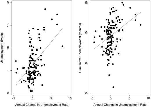
Unemployment events and duration in our analysis sample by business cycle (UR).
Notes: These summary estimates are computed by collapsing the dataset by country and year and estimating the percent of workers who experience an unemployment event and the average cumulative duration of unemployment.
Source: EU-SILC, BHPS, UKHLS, GSOEP, SIPP, 2004–2014.
Table 3 presents regression results for our main models. We start reporting the estimated average unemployment scarring on earnings in our sample. This coefficient should be interpreted as the average earnings loss among workers who lost jobs in this period; more specifically, the difference between within-person earnings change among workers who lost jobs and within-person earnings change among similar workers who did not lose jobs. We find that workers lose about 11% of earnings due to unemployment; their earnings change would have been 11% higher had they not experienced job loss. This estimate is comparable to what previous studies have found (e.g. Gangl, 2006).
Associations between unemployment scarring, EPL and business cycle (UR)
| Variables | Model 1 | Model 2 | Model 3 | Model 4 |
|---|---|---|---|---|
| Constant | −0.114*** | −0.192*** | −0.186*** | −0.170*** |
| (0.0156) | (0.0110) | (0.00773) | (0.0158) | |
| EPL | 0.0374*** | 0.0354*** | 0.0436*** | |
| (0.00830) | (0.00725) | (0.0160) | ||
| UR | −0.00256 | −0.0388** | −0.0398* | |
| (0.00365) | (0.0183) | (0.0209) | ||
| EPL##UR | 0.0154** | 0.0157* | ||
| (0.00736) | (0.00854) | |||
| UI | −0.00299 | |||
| (0.0156) | ||||
| UD | −0.00106 | |||
| (0.00112) | ||||
| Random intercepts | Yes | Yes | Yes | Yes |
| Observations | 130 414 | 130 414 | 130 414 | 130 414 |
| Number of groups | 21 | 21 | 21 | 21 |
Notes: The dependent variable is the estimated individual-level treatment effect from the DiD propensity score matching algorithm, expressed as the difference in logged earnings change between T1 and T3 between the treatment and control group.
Source: EU-SILC, BHPS, UKHLS, GSOEP, SIPP, 2004–2014.
Standard errors in parentheses.
P < 0.01,
P < 0.05,
P < 0.1.
Model 2 adds the two key variables of interest, EPL and UR, and Model 3 adds the interaction term that tests whether the effectiveness of EPL changes under different macroeconomic conditions. Consistent with previous research, we find that EPL protects workers’ earnings losses. A one-unit increase in the EPL scale (EPL scale median is 2, min 0.26 max 3.3), lowers earnings loss by 3%. This translates into a substantial drop from 18% to 15% if we move from 0 to 1 on the EPL scale. Workers who lose jobs in countries with robust employment protection experience lower unemployment scarring than workers who lose jobs in countries with little employment protection. In Model 2, the coefficient for unemployment rate is initially not statistically significant, but Model 3 suggests this is because its effect systematically varies across countries. Model 3 shows that rising unemployment worsens earnings losses especially in weakly regulated labor markets, where a one-unit increase in the unemployment rate is increasing workers earnings losses by as much as 3.5% in the most liberal environment in the sample (in our sample, the lowest EPL level is 0.26 and the model shows the effect when EPL level is set to 0), but this cyclical effect declines in magnitude the more regulated the national labor market.
Model 3 shows that the rate at which macroeconomic conditions affect unemployment scarring is moderated by countries’ EPL level. We find that unfavorable macroeconomic conditions increase unemployment earnings scarring more in countries with weaker employment protections than in countries with stronger employment protections. This result is consistent with the idea that EPL continues to perform well and to protect workers from severe earnings scarring even under deteriorating macroeconomic conditions. This result does not support the critical approach suggesting that EPL is no longer effective in contemporary economies exposed to growing macroeconomic volatility.
It could be that results in Model 3 are biased because they do not account for country differences in UI policies and unionization (UD), both variables that have been previously shown to affect unemployment outcomes (i.e. Gangl, 2006). In Model 4, we add UI and UD as controls and find that EPL and UR main effects and interaction remain largely intact. This bolsters our confidence in the results. Model 4 also shows that neither UI nor UD appears to be associated with unemployment scarring. This is inconsistent with previous studies, which show that UI reduced unemployment scarring (Gangl, 2006). We examined this finding further and concluded that this discrepancy is likely due to the fact that our data represent monthly wages, instead of hourly wages. In supplementary analyses with a subsample where hours of work are available, we find that UI is associated with lower unemployment scarring as previous studies have shown. Sensitivity analyses assessing the robustness of our findings to different matching specifications and methods also confirm our findings. Models including country-fixed effects to assess the sensitivity of our results to unobserved fixed heterogeneity at the country-level also corroborate our findings. We further discuss these results in the additional sensitivity tests section below. In all these analyses, we find that EPL lowers unemployment earnings scarring and that negative macroeconomic conditions increase earnings scarring more in contexts with weak employment protection.
Figure 3 illustrates the interaction between EPL and UR, comparing high- and low-EPL contexts. We select two cutoff points to present the results, the low-EPL scenario represents the lowest EPL level observed in our dataset corresponding to the USA (EPL = 0.26) and the high-EPL scenario corresponds to the highest EPL level observed in our dataset corresponding to Czechia (EPL = 3.3). In countries with robust EPL, unemployment scarring is largely insensitive to changes in macroeconomic conditions. By contrast, in countries with weaker EPL, unemployment scarring is cyclical and becomes larger as macroeconomic conditions deteriorate. In a country with weak EPL, it makes a big difference whether workers lose a job in a context of rising unemployment or not. In a country with robust EPL, the penalty to unemployment does not substantially change when macroeconomic conditions deteriorate.
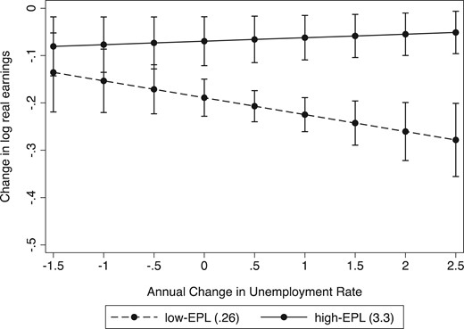
Predicted earnings losses by EPL and business cycle (UR).
Notes: The low-EPL scenario represents the lowest EPL level observed in our dataset corresponding to the USA (EPL = 0.26) and the high-EPL scenario corresponds to the highest EPL level observed in our dataset corresponding to CZ (EPL = 3.3).
Source: EU-SILC, BHPS, UKHLS, GSOEP, SIPP, 2004–2014.
Why is unemployment scarring worse in negative macroeconomic conditions in countries with weak employment protection? Table 4 presents results for the four mechanisms discussed above: reluctance to hire, stigma (uncertainty-related and culture-related), labor market segmentation and wage dispersion. We begin testing the labor segmentation mechanism, which concerns differences in the composition of the unemployed workers across countries that vary by EPL and the possibility that macroeconomic shocks would shift the composition of unemployed workers differently in contexts with strong and weak EPL. For instance, if strong EPL continues to protect ‘insider’ workers in a context of recession because its associated firing costs remain high, a negative macroeconomic environment might increase job losses among highly skilled and high-wage workers relatively more in contexts with weak EPL than in contexts with strong EPL, resulting in greater deterioration of unemployment scarring on earnings in contexts with weak EPL than in contexts with strong EPL. Model 5 tests for this explanation by adding controls for the characteristics of the jobs that are lost including skill level, occupation, job tenure and work hours. The results show that differences in composition do not explain why unemployment scarring deteriorates more in countries with low unemployment protection; EPL and UR main coefficients and the interaction remain largely unaltered. If anything, the interaction is slightly strengthened after controlling for these compositional differences. It is possible in principle that our covariate controls are insufficiently detailed to capture some more nuanced patterns and that we fail to capture how specific compositional shifts play a role in deteriorating unemployment scarring in a context of weak EPL. However, as our empirical results rest on a DiD matching estimator that controls for both observed and unobserved time-constant individual characteristics in a very general way, it seems fair to argue that systematic bias in time-varying unobservables, i.e. in covariates not already incorporated in the analysis, would have to be on some very particular empirical pattern to overturn our fundamental conclusions. Naturally, we have no way of ascertaining more than data limitations permit, and we emphasize that it is possible in principle that some time-varying unmeasured characteristic could affect our inferences on the interaction between EPL and UR. But given the safeguards already implemented in our hierarchical DiD design, we would argue that unobserved compositional mechanisms are very unlikely the primary driver of the interaction between EPL and macroeconomic environment reported here.
Determinants of unemployment scarring, structural and individual-level mechanisms
| Variables | Model 5 | Model 6 | Model 7 | Model 8 |
|---|---|---|---|---|
| Constant | −0.259*** | −0.102** | −0.0853** | −0.129** |
| (0.0376) | (0.0453) | (0.0422) | (0.0624) | |
| EPL | 0.0392** | −0.00166 | −0.0185 | −0.00937 |
| (0.0171) | (0.0139) | (0.0151) | (0.0286) | |
| UR | −0.0468** | −0.0298* | −0.0313* | −0.0327* |
| (0.0192) | (0.0181) | (0.0174) | (0.0194) | |
| EPL##UR | 0.0169** | 0.00857 | 0.00940 | 0.0117 |
| (0.00769) | (0.00698) | (0.00674) | (0.00785) | |
| UI | −0.00524 | −0.00999 | −0.00560 | −0.00198 |
| (0.0161) | (0.0155) | (0.0143) | (0.0150) | |
| UD | −0.000992 | −0.00147* | −0.00146* | −0.000795 |
| (0.00124) | (0.000759) | (0.000858) | (0.00131) | |
| Cumulative unemployment | −0.00757* | −0.0309*** | −0.0317*** | |
| (0.00399) | (0.00514) | (0.00406) | ||
| ##EPL | 0.0107*** | 0.0114*** | ||
| (0.00253) | (0.00224) | |||
| Wage inequality | 0.00421 | |||
| (0.00450) | ||||
| Education | ||||
| Secondary | 0.0158 | 0.0148 | 0.0136 | 0.0154 |
| (0.0233) | (0.0258) | (0.0254) | (0.0260) | |
| College | 0.0299 | 0.0282 | 0.0280 | 0.0294 |
| (0.0206) | (0.0222) | (0.0218) | (0.0213) | |
| 0.0811 | 0.0753 | 0.0754 | 0.0758 | |
| (0.177) | (0.183) | (0.182) | (0.176) | |
| Work hours | 0.00015** | 0.000145** | 0.000148** | 0.000170** |
| (7.43e-05) | (7.37e-05) | (7.40e-05) | (7.59e-05) | |
| Job tenure | −0.000165** | −0.000154** | −0.000156** | −0.00017** |
| (6.86e-05) | (7.33e-05) | (7.38e-05) | (7.09e-05) | |
| Women | 0.0133 | 0.00963 | 0.0103 | 0.0123 |
| (0.0156) | (0.0168) | (0.0166) | (0.0166) | |
| Random intercepts | Yes | Yes | Yes | Yes |
| Random slopes | Yes | Yes | Yes | Yes |
| Observations | 130 414 | 130 414 | 130 414 | 130 414 |
| Number of groups | 21 | 21 | 21 | 21 |
Notes: The dependent variable is the estimated individual-level treatment effect from the DiD propensity score matching algorithm, expressed as the difference in logged earnings change between T1 and T3 between the treatment and control group. All models control for dummy variables for single-digit ISCO occupation codes.
Source: EU-SILC, BHPS, UKHLS, GSOEP, SIPP, 2004–2014.
Standard errors in parentheses.
P < 0.01,
P < 0.05,
P < 0.1.
A second plausible mechanism is related to behavioral responses to job loss from employers that prolong unemployment duration and exacerbate unemployment scarring on earnings (Stevens, 1997). Both the reluctance to hire approach as well as the uncertainty-related unemployment stigma approach suggest this process. If negative macroeconomic environments prolong unemployment duration more in contexts with weak EPL than in contexts with strong EPL, either because the reluctance to hire or the uncertainty-related unemployment stigma being more elastic and increasing relatively more in those contexts, this could explain the greater deterioration of scarring on earnings in contexts with weak EPL. Although long-term unemployment is typically associated with contexts with robust EPL, recent research shows that during the Great Recession long-term unemployment increased across a wide variety of countries (Kroft et al., 2016). Model 6 examines these possibilities by adding a control variable for cumulative unemployment duration that captures both length of unemployment and re-unemployment incidence. We find that the interaction coefficient between EPL and UR loses statistical significance and drops in size, suggesting that cumulative unemployment plays a role in this interaction. The coefficient for cumulative unemployment shows that workers with greater exposure to unemployment also experience greater earnings scarring.
To disentangle whether cumulative unemployment mediates or moderates the relationship between EPL and UR, Model 7 adds an interaction term between EPL and cumulative unemployment. Mediation would imply that the interaction is mainly produced through a compositional effect, i.e. a larger increase in long-term unemployment associated with negative macroeconomic conditions in contexts with low-EPL because unemployed workers become relatively less likely to be rehired in low-EPL countries (either related to reluctance to hire or uncertainty-related unemployment stigma reducing hiring rates and increasing unemployment length). The interaction term addresses the additional possibility that EPL moderates the relationship between long-term unemployment and unemployment scarring by producing higher penalties to long-term unemployment in low-EPL contexts. This could result from either uncertainty-related unemployment stigma mechanisms lowering wage offers to unemployed workers and/or the cultural environment with higher unemployment stigma. EPL can safeguard workers against elevated earnings losses, even when they remain unemployed for a long time, by constraining employers’ bandwidth to set individual wages and discriminate or stigmatize based on workers’ employment history. This is consistent with prior research finding that EPL increases unemployment spell duration but results in better job matches (Gangl, 2004b). Consistent with a moderation mechanism, we find that cumulative unemployment is associated with higher scarring in contexts with weak EPL. This result suggests that the reason why cumulative unemployment explains the interaction between EPL and UR is because the greater prevalence of long-term unemployment associated with periods of high unemployment are more negatively penalized in labor markets with weak EPL than in contexts with robust EPL.
Model 8 examines the final mechanism concerning earnings dispersion, the idea being that higher inequality increases the likelihood of elevated earnings scarring. We find that general wage compression does not change the observed patterns, and it does not notably change the interaction between cumulative unemployment and EPL. Consistent with previous research (Gangl, 2006), these results suggest that it is not general wage compression in the labor market whereby EPL lowers earnings scarring among the unemployed, but, as discussed before in conjunction with Model 6, the fact that stricter EPL indirectly prevents employers to penalize workers for unemployment spells when making wage offers (or offering job conditions more broadly) at reemployment.
Figure 4 illustrates the finding that penalties to cumulative unemployment duration produce a large difference across EPL contexts. We compare workers with short and long cumulative unemployment durations in contexts with low- and high-EPL and across the business cycle. Among workers with short unemployment exposures, increasing unemployment rates worsen unemployment scarring similarly in contexts with weak and robust EPL. Among workers with long exposure to unemployment, however, deteriorating macroeconomic conditions augment earnings scarring in countries with weak EPL but not in countries with robust EPL.
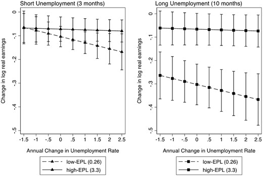
Predicted earnings losses by EPL, unemployment rate (UR) and unemployment cumulative duration.
Notes: The low-EPL scenario represents the lowest EPL level observed in our dataset corresponding to the USA (EPL = 0.26) and the high-EPL scenario corresponds to the highest EPL level observed in our dataset corresponding to CZ (EPL = 3.3).
Source: EU-SILC, BHPS, UKHLS, GSOEP, SIPP, 2004–2014.
4.1 Additional sensitivity tests
We test the sensitivity of our results to alternative measures of macroeconomic conditions and matching estimators. Table 5 replicates key findings substituting the macroeconomic indicator for a measure of change in GDP indexed to pre-recession levels (Models 9 and 10) and using nearest neighbor matching instead of Kernel matching (Models 11 and 12). Our conclusions are robust to these sensitivity analyses using different measurement and matching specifications. Table 5 shows robust evidence of the interaction between EPL and macroeconomic environment, showing that the association between unemployment scarring and macroeconomic environment is stronger in contexts with weak EPL. It also shows robust evidence that cumulative unemployment interacts with EPL and plays a key role explaining the interaction between EPL and macroeconomic environment. Both alternative specifications provide robust evidence that penalties to long-term unemployment are larger in contexts with weak EPL. Once cumulative unemployment is added to the models, the interaction between EPL and the macroeconomic environment is no longer statistically significant.
Sensitivity tests using alternative measures of macroeconomic environment and alternative matching algorithm
| Variables | Model 9 Macroeco indicator = GDP change; Matching = Kernel | Model 10 Macroeco indicator = GDP change; Matching = Kernel | Model 11 Macroeco indicator = UR_CH; Matching = nearest neighbor | Model 12 Macroeco indicator = UR_CH; Matching = nearest neighbor |
|---|---|---|---|---|
| Constant | −0.142*** | −0.158*** | −0.173*** | −0.167*** |
| (0.0247) | (0.0588) | (0.0161) | (0.0514) | |
| EPL | 0.0419*** | 0.00418 | 0.0418** | 0.00725 |
| (0.0157) | (0.0225) | (0.0164) | (0.0218) | |
| UR | −0.0256*** | −0.00740 | −0.0385* | −0.0240 |
| (0.00944) | (0.00841) | (0.0212) | (0.0171) | |
| EPL##UR | 0.00526* | 0.00379 | 0.0153* | 0.00676 |
| (0.00314) | (0.00281) | (0.00863) | (0.00682) | |
| UI | −0.0125 | −0.00234 | −0.00140 | −0.000940 |
| (0.0172) | (0.0138) | (0.0162) | (0.0139) | |
| UD | −0.00113 | −0.000643 | −0.000929 | −0.000728 |
| (0.00108) | (0.000839) | (0.00113) | (0.000786) | |
| Cumulative unemp. | −0.0301*** | −0.0303*** | ||
| (0.00538) | (0.00555) | |||
| ##EPL | 0.0102*** | 0.0103*** | ||
| (0.00254) | (0.00259) | |||
| Wage inequality | 0.00825** | 0.00825*** | ||
| (0.00334) | (0.00303) | |||
| Education | ||||
| Secondary | 0.0193 | 0.0190 | ||
| (0.0276) | (0.0274) | |||
| College | 0.0291 | 0.0305 | ||
| (0.0227) | (0.0225) | |||
| Work hours | 0.000114 | 0.000130** | ||
| (7.49e-05) | (6.55e-05) | |||
| Job tenure | 0.0708*** | 0.0715*** | ||
| (0.0230) | (0.0231) | |||
| Women | 0.0111 | 0.0111 | ||
| (0.0170) | (0.0171) | |||
| Random intercepts | Yes | Yes | Yes | Yes |
| Random slopes | No | Yes | No | Yes |
| Observations | 130 414 | 130 414 | 130 414 | 130 414 |
| Number of groups | 21 | 21 | 21 | 21 |
Notes: The dependent variable is the estimated individual-level treatment effect from the DiD propensity score matching algorithm, expressed as the difference in logged earnings change between T1 and T3 between the treatment and control group. All models control for dummy variables for single-digit ISCO occupation codes.
Source: EU-SILC, BHPS, UKHLS, GSOEP, SIPP, 2004–2014.
Standard errors in parentheses.
P < 0.01,
P < 0.05,
P < 0.1.
In supplementary analyses available in the Online Appendix, we tested the sensitivity of our findings to survey design and interview timing (Supplementary Table S3), we included country fixed effects to examine sensitivity to country-level fixed unobserved heterogeneity (Supplementary Table S4), and we reran the analyses excluding key countries from our analysis sample (i.e. the USA and Germany; Supplementary Table S5). With few minor discrepancies in tests of statistical significance, all these results replicate the substantive patterns presented here and confirm the robustness of our findings. The results show that the interaction between cumulative unemployment and EPL is key to explain the negative interaction between EPL and the macroeconomic environment; in other words, that unemployment scarring in deteriorating macroeconomic conditions is worse in a context with weak EPL and that this is because long-term unemployment is more strongly penalized in these contexts.
5. Discussion
The Great Recession renewed interest in critiques of EPL, arguing that EPL curtails much-needed flexibility necessary to adjust to an increasingly volatile macroeconomic environment, hurting workers’ economic prospects as a result. This article has focused on unemployment scarring on earnings to examine this claim. By studying how unemployment scarring on earnings varies across EPL and macroeconomic environments, we update results from previous research that analyzed these two context-level variables separately and provide a novel test about the interaction between the two. Contrary to critics of EPL, we find that negative macroeconomic conditions worsen unemployment scarring on earnings more in contexts with weak EPL, while workers in contexts with robust EPL remain protected. Our research also confirms previous studies showing that unemployment scarring on earnings is smaller in contexts with EPL and higher under negative macroeconomic conditions. Taken together, our study finds no evidence that EPL is detrimental for workers, neither in a context of economic growth, nor in a context of macroeconomic turbulence.
Our results show that severe penalties to long-term unemployment are a central mechanism worsening unemployment scarring during economic recessions in contexts with weak EPL. We find that earnings scarring for long-term unemployed workers are much higher in contexts with weak EPL. Thus, although the Great Recession increased the prevalence of long-term unemployed workers across the board (Kroft et al., 2016), only in contexts with weak EPL did unemployed workers experience large increases in earnings losses and earnings scarring. To the extent of our knowledge, no prior research has directly reported systematic variation in penalties to long-term unemployment across policy contexts. While research has focused on how EPL generates barriers to reemployment (Dieckhoff, 2011), only a few studies have emphasized that this delay does not come with increases in earnings losses (Gangl, 2004a, 2006). The finding that EPL is associated with lower unemployment scarring for those who experience long-term unemployment is consistent with approaches that emphasize both structural and cultural features of EPL, in particular, the constraints on employers’ ability to set individual wages and discriminate based on workers’ prior work history as well as a cultural environment that lowers unemployment stigma. All of these structural components offer plausible explanations for how EPL lowers earnings scarring even among the long-term unemployed and in a situation of macroeconomic uncertainty.
Although critics of EPL stress the potentially adverse effects of employment rigidity in a context of macroeconomic volatility (i.e. European Commission, 2012), the finding that workers fare worse under market volatility in contexts with weak EPL is entirely consistent with research reporting greater market exposure and vulnerability under liberal policy regimes (DiPrete et al., 1997). Our results add to the skepticism that scholars raise about mainstream economic policy lines critical of EPL without robust evidence (i.e. Avdagic and Salardi, 2013; Hastings and Heyes, 2018). Some mainstream economic theories frame unavoidable tradeoffs between economic performance and market coordination institutions, often ignoring evidence about multiple equilibrium regimes that provide a more complex picture about socioeconomic outcomes (Estevez-Abe et al., 2001). This speaks to the importance of conceptual frameworks that integrate multiple processes and examine the interrelationship between them (Gangl, 2006; Biegert, 2017). The four mechanisms analyzed here are interrelated and are not mutually exclusive. Employer reluctance to hire or uncertainty-related unemployment stigma, for instance, are related to labor market segmentation in that hiring costs will systematically differ between insider and outsider workers. Wage inequality, too, can shape employer hiring costs assessments and hiring decisions. Our analysis has sought to provide a comprehensive framework and operationalize each mechanism separately, but future research should further examine the relationship between these mechanisms.
There are several limitations to the analyses presented here. First and foremost, our analyses can only speak to unemployment earnings scarring in the short-term and among attached workers who lose jobs. This limited scope excludes labor market entrants and long-term earnings scarring, both of which may have different implications for the interaction between EPL and macroeconomic environments. Data limitations, in particular the 4-year rotating panel structure, make it impossible for us to examine long-term earnings scarring. Prior research found that countries differ more in short-term penalties than in long-term penalties, with long-term penalties attenuating the cross-country variation (DiPrete and McManus, 2000; Gangl, 2006). This suggests that our conclusions might not change dramatically if we included long-term scarring. More research is necessary to investigate how long-term penalties vary with the macroeconomic environment. Similarly, more research is needed to investigate how the interaction between EPL and macroeconomic environment operates for labor market entrants. Second, our research design prioritized coverage (countries and years) and this comes with costs for measurement precision. We estimate monthly earnings measures from annual earnings reports and this introduces measurement error into our estimates. We face similar challenges to measure job characteristics, like detailed occupation or tenure length. Data availability also limits the kinds of macro-level variables we can incorporate in our models; for instance, we are unable to use more specific macroeconomic indicators, such as vacancy rates, because they are not available for most countries and years in our dataset. These measurement limitations can have a negative impact on both our matching analysis as well as on our regression analyses. While improvements in these measurement issues would definitively refine our estimates, sensitivity tests with alternative measurement and specification make us confident that our findings are robust. Also, because we implement a DiD matching estimator, our analyses control for both observed and unobserved fixed individual characteristics and these measurements limitations only apply to time-varying characteristics.
The results in this article have implications for contemporary debates about labor market institutions and economic performance. We find robust evidence that EPL lowers unemployment earnings scarring both in a context of economic downturn as well as in a context of economic growth. These findings challenge critics’ hypothesis that EPL would amplify the negative consequences of economic downturns on workers, and favors continued support for EPL. It is possible, however, that EPL amplifies other negative consequences of economic downturns that are not examined here. Future research should investigate the interaction between labor market institutions and macroeconomic environment for additional populations and outcomes to contribute to this debate.
Supplementary material
Supplementary material is available at Socio-Economic Review Journal online.
Footnotes
For more information, see http://www.oecd.org/employment/emp/oecdindicatorsofemploymentprotection-methodology.htm
In sensitivity analyses reported in Table 4, we confirm the robustness of our conclusions to an alternative indicator of macroeconomic environment measuring change in GDP indexed at pre-Great Recession levels.
Some of the control variables entered in this model are also variables included in the propensity score model. While the propensity score model step aims to obtain an average treatment effect (i.e. a weighted regression estimate based on the matched treatment and control sample), these subsequent regression models aim to describe the distribution of treatment effects, or treatment heterogeneity, across individual characteristics (Xie et al., 2012).
Acknowledgements
This research was carried out in part using the facilities of the University of Pennsylvania Population Studies Center (R24 HD044964). We thank Eurostat, the United States Census Bureau, the Institute for Social and Economic Research (ISER) at the University of Essex and the German Institute for Economic Research (DIW) for making available the EU-SILC, SIPP, BHPS, UKHLS, and SOEP datasets used in this research. Of course, the data providers are not responsible for any aspect of our analysis or for our interpretation of results. An earlier version of this article was prepared for presentation at the 2016 meetings of the American Sociological Association in Seattle, Washington. We are grateful to Kristina Lindemann, Carlotta Giustozzi, Jan Brülle, Timo Lepper, Rona Geffen, Anne Kronberg, Fabian Ochsenfeld, and the SER reviewers for their helpful comments and suggestions on earlier drafts. The authors are not aware of any conflict of interest that would affect the conclusions expressed in this research.
Funding
This research has been supported by the European Research Council under the European Union’s Seventh Framework Programme (FP7/2007-2013, ERC grant agreement n° ERC-2013-CoG-615246-CORRODE). Of course, the data providers are not responsible for any aspect of our analysis or for our interpretation of results.
References
European Commission (
European Commission (
European Commission (
European Commission (
OECD (
OECD (
