


Abstract
We exploit a variation in organizational hierarchy induced by a reorganization plan implemented in roughly 2,000 bank branches in India. We do so to investigate how organizational hierarchy affects the allocation of credit. We find that increased hierarchization of a branch induces credit rationing, reduces loan performance, and generates standardization in loan contracts. Additionally, we find that hierarchical structures perform better in environments characterized by a high degree of corruption, highlighting the benefits of hierarchies in restraining rent-seeking activities. Overall, our results are consistent with the view that valuable information may be lost in hierarchical structures.
Received May 4, 2018; editorial decision April 30, 2018 by Editor Itay Goldstein. Authors have furnished an Internet Appendix, which is available on the Oxford University Press Web site next to the link to the final published paper online.
Over recent years, there has been a substantial change in the lending landscape, with banks becoming larger, more globalized, and more complex (Mester 2012; Herring and Carmassi 2012). While there is evidence that banks might benefit from economies of scale (Focarelli and Panetta 2003), it is argued that hierarchical structures may be inferior when it comes to granting loans to small and medium sized enterprises (Stein 2002). Given the importance of small and entrepreneurial firms for innovation and economic growth, it is plausible that the shift toward hierarchical organizations hampers growth. In this paper, we examine how organizational hierarchy affects the allocation of credit.
There is now growing recognition that organizational design matters (Radner 1993; Bolton and Dewatripont 1994; Aghion and Tirole 1997; Garicano 2000; Dessein 2002). However, despite the abundance of theoretical literature on this topic, empirical research has been rather scant.1 Two obstacles hinder empirical research in this area. The first impediment comes from the paucity of good micro-level data. A researcher not only needs detailed data on the organizational design of banks, but also requires comprehensive information on outcome variables, to identify the effect of changes in organizational design. The second problem relates to the classic endogeneity problem. Even if one is fortunate enough to gain access to organizational-level micro data, one still has to grapple with the fact that the choice of organizational design is not random. While cross-sectional studies are informative about the plausible relationship, they are plagued by the problem of omitted variables. To make any causal claims, the researcher has to seek some exogenous variation in the organizational hierarchy.
In this paper, we use micro-level data from a large bank in India with roughly 2,000 branches, to examine how organizational hierarchy affects lending. The data set offers not only comprehensive information on financial contracts of individual borrowers but also micro-details on the organizational design of all branches of the bank. In particular, it provides a measure of organizational hierarchy: the number of managerial layers within a bank branch, where more layers capture a greater degree of hierarchization.
We exploit changes in the organizational design, brought about by a bank-level, predetermined reorganizational rule, and a difference-in-differences (DID) research design. Specifically, a branch receives an upgrade if its total business (deposits and loans) exceeds a certain threshold for eight quarters in a row. The reverse is true for a downgrade. The upgrade adds a new managerial layer to a branch office – the branch is now headed by a more senior manager, who by virtue of her seniority in the bank can approve larger loans. Thus, the upgrade generates two simultaneous affects. The addition of a new layer increases the hierarchical distance for smaller loans. The opposite is true for larger loans that can be approved internally after an upgrade due to the higher loan approval limit of the more senior manager. To allow for comparability, our experiment examines whether the lending behavior for loans that can be approved in the lowest managerial layer changes with the addition of another managerial layer.2
The following example illustrates the empirical strategy of the paper. Consider a level 2 branch that is upgraded to a level 3 branch. Further assume that the level 1 branch has the authority to approve loans below USD 5,000, the level 2 branch has the power to approve loans up to USD 10,000 and the level 3 branch has an approval limit of USD 20,000. Any loan above these limits would have to be sent to a higher level regional office3 for its approval, as it falls outside the branch’s loan approval limits. We compare how the lending behavior of a bank branch changes with the hierarchization for loans that are below the USD 5,000 threshold. To control for time trends and other omitted factors, our control group is another bank branch of the same bank in the same district in the same quarter.4
Existing theories posit that the cost of communicating and transmitting information increases with hierarchization (Radner 1993; Bolton and Dewatripont 1994; Aghion and Tirole 1997; Garicano 2000; Dessein 2002; Stein 2002). To the extent that hierarchy impedes information production (Stein 2002), it is natural to expect implications on bank lending. While the effect of information on lending can be rather subtle, the canonical models of credit argue that improving information in credit markets facilitates lending and broadens access to finance (Stiglitz and Weiss 1981). Because decentralization in decision-making increases banks’ ability to generate information, we expect there to be more lending (i.e., less credit rationing) in decentralized structures. In a similar vein, it is natural to expect that better information would allow banks to target credit to more profitable projects and away from less profitable ones, thus increasing the overall profitability of their portfolio. Furthermore, to the extent that better information allows the banks to discriminate between borrowers, one would expect a greater dispersion in loan contract terms (Cornell and Welch 1996; Cerqueiro et al. 2010; Rajan et al. 2015).
We find that organizational hierarchy affects both the quantity and the quality of loans originated by the bank. Specifically, we observe that an increase in hierarchy results in a 9.9% decline in total new loans issued by the bank branch and a 5.4% decline in the average loan size. Furthermore, we find that an increase in organizational hierarchy leads to a 4.5% reduction in the number of small retail borrowers. On examining the performance of these loans, we find that there is a substantial drop in the quality of loans after a branch becomes more hierarchical. Delinquencies of loans are 30% higher, and returns 15% lower. Overall, our results support the view that better information is generated in more decentralized branches.
To further sharpen our analysis, we examine the second moment of contract terms on loan agreements, in a similar spirit to Rajan et al. (2015).5Rajan et al. (2015) argue that an increase in information should increase the variance of the contract terms, as it allows banks to discriminate amongst borrowers. With better information, banks can target credit to more profitable borrowers and away from less profitable ones (to weed out bad borrowers). Consistent with this prediction, we find that a new layer in the hierarchy reduces the variance of contract terms (loan size) and generates contract standardization.
As pointed out above, higher level branches are headed by more senior managers, who have the authority (granted by the central office) to approve larger loans. Thus, these “large” loans are approved internally after an upgrade. We find that after hierarchization, a branch issues more of the “large” loans and generates more information on them. Given that these loans underwent a reduction in organizational distance, the results provide additional support for the view that an increase in organizational hierarchy reduces the information produced on loans.
This generates an interesting trade-off for the branch. While the upgraded branch loses out on small loans, it gains on larger loans that are now processed inside the branch. Interestingly, however, we find that the gains in large loans do not offset the losses on small loans. To assess the overall effect of branch-level reorganizations, however, one has to evaluate the profitability of the bank. Because upgrading a branch frees up resources at regional or higher level offices, these offices can be more effective in other bank-level assignments, such as business development and risk management. Our analysis focuses on only branch-level profitability, and not on the overall profitability of the bank. It should be noted, however, that during our sample the profitability of the bank increased. In addition, the bank opened new branches in 43 previously unbanked districts, thereby allowing it to access new markets. Thus, the overall effect for the bank is likely to be positive. Because we do not have a control group for the bank-level analysis, we refrain from making any causal claims on the overall profitability of the bank.
Next, we investigate how organizational hierarchy interacts with corruption. Delegation in the presence of corruption may be a double-edged sword (Tirole 1986; Banerjee et al. 2013). Delegation provides an extra incentive for an agent to perform a task. However, when the agent’s incentives are not aligned with those of the principal, it may be worthwhile taking this discretion away. To understand how organizational hierarchy interacts with rent extraction, we compare the effects in more corrupt states to those in less corrupt ones. Our proxy for corruption is provided by Transparency International. The index is particularly useful for our study, because it examines corruption in banking services. It measures the fraction of respondents who actually paid a bribe for obtaining these services. The study points out that the majority of these bribes were paid to secure a loan.6 Our estimates indicate that for corrupt states the effects of hierarchization are significantly reduced, highlighting the benefits of hierarchical structures in corrupt environments.
Results thus far are consistent with the view that an increase in organizational hierarchy adversely affects lending. However, it is plausible that other contemporaneous changes may have affected lending. As a first check, we confirm that our results remain strong after controlling for local shocks to credit demand within the same district and the same city.7 We also verify that our results are not driven by changes in branch managers. We carry out many other robustness tests and discuss some alternative stories in Section 6.
This paper adds to the literature on organizational hierarchy and information production. Theories in this area can be broadly categorized into one of two strands. The first one deals with information transmission in teams with incentive conflicts (Aghion and Tirole 1997; Stein 2002). The second one examines information processing in teams without incentive problems. These theories argue that hierarchy might be inferior, when communicating and processing information is very costly (Bolton and Dewatripont 1994; Garicano 2000). Both sets of theories predict that organizational hierarchy might lead to difficulties in processing and communicating information. This paper documents that organizational hierarchy leads to distortions in information production, but it is silent about which of the two classes of theories generates our results.
Our work is closest to Liberti and Mian (2009) and Liberti (2017), who show that more hierarchical organizational structures tend to rely more heavily on objective rather than subjective information.8Liberti et al. (2015) examine how banks change their organizational design in response to a change in external information with the introduction of a credit registry. Canales and Nanda (2012) document that banks with less discretionary power at branch offices are less responsive to the competitive environment. Qian et al. (2015) find that when the loan approval is delegated to an individual rather than a committee, the information quality improves. Finally, Cerqueiro et al. (2010) study whether higher dispersion in interest rates is consistent with more discretion in loan approval.9 We complement these papers by examining how a change in organizational hierarchy affects banks’ ability to generate information and to allocate credit. Furthermore, we provide new insights by highlighting some of the benefits associated with hierarchies in corrupt areas.
Our paper also contributes to the literature on distance in credit markets. These studies argue that the proximity between the borrower and the lender mitigates the information asymmetry (Petersen and Rajan 1995; Petersen and Rajan 2002; Degryse and Ongena 2005; Mian 2006; Liberti and Mian 2009; Alessandrini et al. 2009; Agarwal and Hauswald 2010; Brown et al. 2012; Berg et al. 2013; Fisman et al. 2017). The key distinction here is that we focus on hierarchical distance, as opposed to geographical distance (Petersen and Rajan 2002) or cultural distance (Fisman et al. 2017).
1. Theoretical Motivation
In this section, we briefly discuss the main theories with implications on organizational hierarchy and information. The first set of models considers information processing and communication in teams without incentive problems. Generally, these theories argue that organizational hierarchy is less attractive when communication costs are large. Bolton and Dewatripont (1994) consider an environment where a firm trades off gains from specialization against costs of communication.10 In their model, specialized agents collect information that is then communicated to the decision maker. If the costs of communication are high, specialization becomes less attractive. Similarly, Garicano (2000) considers knowledge based hierarchies. In his model, higher layers are solvers of complex problems, while lower layers are routine problem solvers. He proposes a trade-off between the cost of communication (matching a problem with the problem solver) and the cost of acquiring knowledge (the front line can pick up necessary skills and problem solvers are not necessary). If the costs of communication outweigh the costs of acquiring information, hierarchy is less attractive.
The second set of models analyzes information processing in teams with incentive problems. Aghion and Tirole (1997) and Stein (2002) argue that organizational hierarchy creates an ex ante disincentive to collect information. In their model, the subordinate is responsible for collecting information to be transmitted to the manager. Because the manager makes the final decision, there is a positive probability that the suggestion of a subordinate will be overruled. This likelihood of interference dulls the subordinate’s incentive to exert effort in collecting information ex ante. A similar point is raised by cheap talk models (most notably, Crawford and Sobel, 1982, Dessein, 2002). The informed agent sends a signal to a principal who will act on it and affect the welfare of both. If their incentives are misaligned, the agent is prone to misreport the true quality of their project. In this spirit, Harris and Raviv (1998) exploit the cost of auditing the information that is submitted by a subordinate. If the audit costs are very high, the decision will be delegated to the subordinate. In other words, hierarchy becomes less attractive in the presence of high audit costs and misaligned interests.
The effect of information on lending is rather complex. The cannonical models of credit predict that better information on borrowers facilitates lending and broadens access to finance (Stiglitz and Weiss 1981).11 However, the effect of information on overall profitability is less ambiguous. Better information on borrowers allows a bank to target loans to more profitable projects and away from less profitable ones, thereby increasing overall profitability. In addition, Cornell and Welch (1996) and Rajan et al. (2015) argue that better information is likely to increase the variance on loan contract terms, because the bank can use the extra information to increase lending to creditworthy borrowers and reduce lending to riskier borrowers.
In this paper, we document that organizational hierarchy affects lending. It should be noted that while we interpret our results through the lens of the two sets of organizational theories described above, the paper is not a horse race between them.
2. Data
The data for this study come from a large, state-owned Indian bank operating over 2,000 branches. The data set is rich in detail. It contains detailed information not only on all loan contracts but also on the organizational design of all of the bank’s branches.12 At the contract level, it includes the loan balance outstanding, the interest rate, the maturity, the type of collateral, the collateral value, and the number of days late in payment, among other information. On the organizational front, it provides us with information on the number of managerial layers in each branch office, the overall seniority of each manager and their loan approval limit. The sample spans 29 quarters from 1999 Q1 to 2006 Q1.
2.1 Loans and borrowers
We focus on first-time, individual (retail) borrowers. During our sample, the bank issued 1.75 million such contracts. For the purposes of this study, we aggregate the loan-level information and obtain 54,079 branch-quarter observations. In Table 1, we present means, medians, standard deviations, and the 1st and the 99th percentiles for the main variables of interest. The loan amounts are expressed in rupees.13
Summary statistics
| Mean | SD | p1 | p50 | p99 | |
|---|---|---|---|---|---|
| Branch-quarter statistics (N=54,079) | |||||
| New credit (1,000s of rupees) | 1,175.1 | 2,063.4 | 31.0 | 726.4 | 6,650.1 |
| Mean loan amount (1,000s of rupees) | 56.0 | 43.5 | 7.8 | 42.8 | 216.5 |
| # of borrowers | 24.5 | 39.1 | 2.0 | 15.0 | 143.0 |
| Fraction of borrowers delinquent within a year | 0.050 | 0.111 | 0.000 | 0.000 | 0.500 |
| Fraction of debt delinquent within a year | 0.042 | 0.111 | 0.000 | 0.000 | 0.570 |
| Return on loans (value-weighted) | 0.070 | 0.079 | -0.244 | 0.083 | 0.150 |
| Interest rate | 0.11 | 0.018 | 0.082 | 0.116 | 0.158 |
| Maturity (years) | 4.15 | 2.26 | 0.60 | 4.00 | 11.11 |
| Collateral-to-loan (median) | 6.75 | 406.98 | 0.00 | 1.42 | 19.12 |
| SD debt (1,000s of rupees) | 57.6 | 44.7 | 2.3 | 47.9 | 184.1 |
| IQR debt (1,000s of rupees) | 54.6 | 66.8 | 0.7 | 28.2 | 309.8 |
| Branch level | 1.4 | 0.6 | 1 | 1 | 3 |
| Branch level (treated) | 1.7 | 0.7 | 1 | 2 | 3 |
This table reports branch-quarter summary statistics of new individual loans. The variable Branch level is a number between 1 and 3, where the lowest value (level 1) and the highest value (level 3) characterize the least hierarchical branches and the most hierarchical branches, respectively. We report the mean, standard deviation, the 1st percentile, median, and the 99th percentile for all the variables.
In a quarter, the average branch lends to 24 new retail borrowers, with a mean loan size of 56,000 rupees (roughly USD 1,300). Furthermore, the equally weighted delinquency rate, defined as 60 or more days late in repayment within a year after the origination of the loan, is 5.0%. In comparison, the value-weighted delinquency rate is only 4.2%, suggesting that larger debt is less likely to be late in repayment and is issued to better quality borrowers. In addition, the average value-weighted return on loans is 7.0%. Moreover, 90% of all loans are secured with a median ratio of collateral to loan value of 1.42. Finally, the average maturity and interest rate are 4.2 years and 11.4%, respectively.
2.2 Organizational design
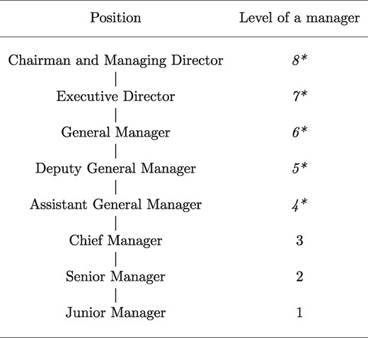
Figure 1 provides an illustration of the managerial hierarchy of the bank. In total, there are eight management levels. Employees in each layer are comparable in terms of their responsibilities, discretionary power as defined by their maximum loan approval limit, experience, and salary. The top five layers, starting with Assistant General Manager, constitute the senior management team. While they are mainly involved in business development, they also originate large loans. The lower ranked employees consist of junior managers, senior managers and chief managers who focus more on the operation side of lending as managers in branch offices. Every ranked employee has a credit origination limit, and that limit increases with the rank of the official.
Organizational design
The bank’s organizational design consists of the eight layers described in the figure. A higher-ranking manager has more decisional power and authority. The top-five layers, marked with an asterisk, are the senior management team, mainly involved in business development. The lower three focus on the operational side of lending.
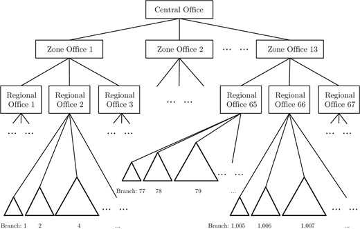
The organizational chart of the bank is as follows (see Figure 2): The Chairman and the Executive Directors of the bank operate from the central office and set all bank-wide policies, which are then executed in other lower-level branches. Zonal offices, which represent distinct geographical zones across the country, operate under the central office. Within each zone, several regional offices are responsible for business development in different regions of a zone. Finally, under each regional office, a large number of standardized branch offices (2,000+) exist and are headed by different levels of managers.
Internal organizational design
The figure shows a schematic illustration of the bank and its branches. Each level has a specified approval limit on the size of the loan. If the loan falls outside of the branch manager’s limits, it is sent to the regional, the zonal, or the head office for approval, depending on the size of the loan.
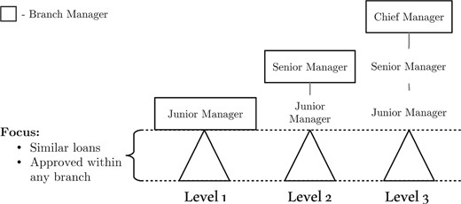
For the organizational design of branches, the branch head can be seen as the chief executive of the branch. They are responsible for the whole business of the branch, within the policy guidelines that are set by the central office. The branch manager can decide on whether to grant a loan and has considerable discretion over the terms of the loan contract, with the exception of the interest rate, which is set by the central office. For instance, all home improvement loans have the same interest rate as car loans with a maturity of up to 5 years (see, for example, Internet Appendix Table A1). In total, there are three branch structures (see Figure 3). The smallest branch (level 1) is typically headed by a junior branch manager, the next branch up (level 2) is headed by a senior branch manager, and finally the branch on level 3 is overseen by a chief manager. Higher-level branches have more layers of hierarchy associated with them. For example, in level 1 branches, branch managers directly interact with the borrowers. However, a level 3 branch would have three layers: junior managers, senior managers, and a chief manager. It should be noted that while the loan officers (or junior managers in our setting) in a branch can approve loans that are within their approval limit, the senior-level manager (if there is one in that branch) can overrule those decisions.
Branch office design
The figure shows a schematic illustration of the bank’s branches. Each level has a specified approval limit on the size of the loan. If the loan falls outside of the branch manager’s limits, it is sent to the regional, the zonal, or the head office for approval, depending on the size of the loan. Our sample consists of three organizational designs: decentralized (level 1), medium hierarchy (level 2), and centralized (level 3). The more hierarchical the branch, the higher the approval limits of its manager. Our analysis focuses on all new individual loans eligible for approval at any organizational design, that is, the loans that fall below the limit of the least hierarchical branch (the triangles at the bottom of the chart).
The lending process is relatively simple (see Figure 4). The borrower approaches the bank and fills in the application form. The application may be rejected by the loan officer, which ends the whole process. If not, the loan officer evaluates the loan application to assess the borrower’s credit risk. The loan officer and the borrower then meet to discuss the needs, collateral requirements and other possibilities. Once a loan officer and a borrower agree on the loan terms, the loan is approved by the loan officer (junior manager) if the agreed size of the loan falls within their discretionary powers (i.e., below 500k rupees). If the loan exceeds the loan officer’s approval limit, it goes to the next authority up for approval. If the requested loan is above the discretionary powers of the branch manager, the loan application, along with the branch’s assessment, is forwarded to a more senior manager in a regional, a zonal, or a central office. Nevertheless, the decision on whether to reject the application or send it for approval outside the branch remains with the head of the branch. On average, a loan application is assessed within 10 days when approved within a branch. The assessment period increases to 2 months when evaluated externally, because the credit files were mailed using postal services during our sample period.

Loan approval process
The flowchart describes the loan approval process. It starts with a loan application at the branch office and continues until the loan is approved or rejected at either the branch or another external office.
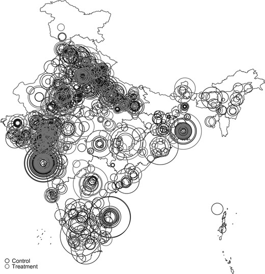
In terms of the geographic distribution, the bank is highly dispersed across India (Figure 5). We created a spatial map and calculated distances between branches, to better understand the market structure. Specifically, for a level 1 branch, the closest levels 2 and 3 branches are 23 and 90 kilometers away, respectively (see Table 2). For a level 2 branch, the closest level 3 branch is 73 kilometers away. On average, there are 1.67 branches per city. Out of all cities, 52% (or 1,396) have only one branch of the bank. Similarly, we find that there are 1.38 branches per ZIP code and 1.38 branches per banking area, as defined by the Reserve Bank of India.14 57% of ZIP codes (1,527) and 66% of banking areas (1,844) have a single branch of this bank. It is worthwhile to note that transportation in India, particularly in rural areas, is not very well developed. The 20-kilometer distance can come at a considerable travel cost.15 As a rule borrowers have to apply at their nearest branch.16
Geographical distribution of branches, weighted by total lending
The center indicates the location of the branch by postal code. The size corresponds to the total amount lent in the branch in 2006.
Distance to the closest branch within the bank
| Branch hierarchy | Regional office | Zonal office | ||||
|---|---|---|---|---|---|---|
| 1 | 2 | 3 | ||||
| Hierarchy | ||||||
| 1 | 12.08 | 22.79 | 90.03 | 131.46 | 204.48 | |
| 2 | 15.47 | 18.18 | 73.82 | 116.25 | 193.08 | |
| 3 | 7.23 | 6.70 | 28.12 | 54.14 | 178.38 | |
| Branch hierarchy | Regional office | Zonal office | ||||
|---|---|---|---|---|---|---|
| 1 | 2 | 3 | ||||
| Hierarchy | ||||||
| 1 | 12.08 | 22.79 | 90.03 | 131.46 | 204.48 | |
| 2 | 15.47 | 18.18 | 73.82 | 116.25 | 193.08 | |
| 3 | 7.23 | 6.70 | 28.12 | 54.14 | 178.38 | |
The table reports the average spatial distance in kilometers to the closest branch, regional office, or zonal office of the same bank. The location of branches is at the ZIP code level. Each row corresponds to the hierarchy of each branch from which the distance is calculated. For instance, for a branch with hierarchy 1, the closest branch with hierarchy 2 is 22.79 kilometers. For a branch with hierarchy 1, the average distance from regional and zonal offices is 131.46 and 204.48 kilometers.
Table 3 reports the summary statistics by branch level. As can be seen from panel A, more hierarchical branches originate larger loans, serve fewer customers, and their loan book performs better, as measured by both delinquencies and returns. Hierarchical branches, however, are more likely to be located in metropolitan areas. Because borrowers might differ in terms of their size and profitability across geographical locations, a simple cross-sectional analysis could capture the heterogeneity of clientele, degree of competition, or other omitted variables rather than organizational design. In panel B, we restrict the sample to only metropolitan areas and find that branches are fairly similar across all levels.17 Our empirical strategy employs a difference-in differences research design to control for these omitted factors.
Summary statistics: Cross-section
| Fraction of debt | ||||||||
|---|---|---|---|---|---|---|---|---|
| Mean loan amount | # of borrowers | del. within a year | Return on loans | |||||
| Branch level (# Obs) | Mean | SD | Mean | SD | Mean | SD | Mean | SD |
| A. All areas | ||||||||
| Level 1 (34,068) | 46,303 | 35,698 | 24.65 | 30.48 | 0.046 | 0.116 | 0.066 | 0.083 |
| Level 2 (17,139) | 70,231 | 48,438 | 25.27 | 52.53 | 0.039 | 0.105 | 0.074 | 0.073 |
| Level 3 (2,872) | 85,918 | 57,944 | 17.94 | 35.20 | 0.024 | 0.083 | 0.078 | 0.067 |
| B. Metropolitan areas | ||||||||
| Level 1 | 90,169 | 60,584 | 13.65 | 14.89 | 0.034 | 0.107 | 0.084 | 0.067 |
| Level 2 | 87,127 | 59,267 | 13.31 | 13.76 | 0.034 | 0.104 | 0.081 | 0.078 |
| Level 3 | 92,702 | 63,363 | 12.06 | 15.27 | 0.022 | 0.083 | 0.080 | 0.071 |
This table reports branch-quarter summary statistics of new individual loans across organizational designs. Panel A considers all geographic areas, and panel B considers only metropolitan areas. The variable Branch level is a number between 1 and 3, where the lowest value (level 1) and the highest value (level 3) characterize the least hierarchical branches and the most hierarchical branches, respectively. We report the mean and the standard deviation for all the variables.
2.3 Employee incentives
Managers are evaluated annually, based on a range of criteria. These include quantitative measures such as the amount and profitability of lending, as well as qualitative considerations such as employee skill development and effective customer communication. These managers are held accountable for loan defaults even after moving branches, on average up to 3 years. After that the responsibility is transferred to a manager at the branch where the loan was originated.
While there is limited incentive pay, managers are motivated through the possibility of promotion to a higher rank or a better posting. Successful managers may be sent to locales with more or better perks such as higher pay (overseas), a larger house, a company car, or control over a larger portfolio (large branches). In a similar vein, poor performers might be moved to less desirable places, which have a weak infrastructure and poor schools. Accordingly, managers have strong incentives to issue profitable loans and score high on other qualitative dimensions that affect their annual evaluations.
3. Empirical Specification
Our identification strategy employs a branch restructuring policy that is driven by predefined rules. A given branch is upgraded (downgraded) if over the last 2 years, the average outstanding balance of the combined loans and deposits exceeds (falls below) a fixed cutoff. In the event of an upgrade, a branch is allocated more resources, including more personnel to meet the rising demand for services in that district, and vice versa. The branch’s organizational hierarchy is also changed to resemble other branches on the same organizational level (see Figure 6). Because managers in a more senior level can approve larger loans, we focus on loans that are below the lowest approval limit, that is, that of junior managers. Therefore, our experiment examines whether the lending behavior for loans that can be approved in the lowest managerial layer changes with the addition of another managerial layer. During our sample period, roughly 500 of all branches were reorganized.
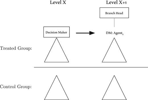
Identification strategy
The figure describes our difference-in-differences (DID) identification strategy. We estimate the effect of organizational design on a set of loans eligible for approval both before and after the treatment. Each quarter, the treatment group consists of all branches that are reorganized. Then we compare our estimated effect on the treatment group with the results of similar branches whose organizational design was left unchanged (control group).
We wish to highlight a few points about the reorganization of branches. First, these cutoffs were fixed in the central office by a new CEO of the bank, before the start of our sample. Thus, from the perspective of a single borrower, the organizational design of a branch is exogenous. Second, we again stress that we are examining the loans that are eligible for internal approval within all branches, that is, we are looking at loans of under 500,000 rupees (approx. USD 11,000). This allows us to analyze a similar set of loans across all types of organizational levels, ensuring that the approval limit does not interfere with the loan decisions. It is important to emphasize that most of the branches that we examine have loan approval limits that are significantly above this cutoff (more than double), so this constraint is not binding for most of the loans that we examine.
Our empirical strategy attempts to identify the effect of organizational hierarchy on the parameters of interest (e.g., contract standardization, delinquencies, or return on loans). We employ a difference-in-differences (DID) strategy and compare branches that were subject to a change in their organizational design against a control group of branches that were not affected by these reorganizations. Thus, the empirical specification is given by
where the dependent variable (e.g., defaults) is measured at the branch-quarter level; |$q$| and |$b$| index the quarter and the branch, respectively. |$Branch~level_{bq}$| stands for the organizational design of branch |$b$| in quarter |$q$|. It is a number between 1 and 3, where the lowest and highest values describe decentralized and hierarchical (i.e., four-layer) branches, respectively. The branch fixed effects |$\left(\tau_{b}\right)$| absorb any time invariant branch characteristics. The quarterly dummies |$\left(\tau_{q}\right)$| control for aggregate time trends. This strategy identifies the effect of organizational structure on the credit market outcomes, controlling for time and branch invariant effects. The coefficient |$\delta$| is our DID estimate of the effect of organizational hierarchy on, for example, the default rates.
A concern might be that some credit demand shocks coincide with the reorganization of branches. We control for this by including district-quarter fixed effects.18 In such a specification, one compares the default rates of a reorganized branch against a branch that was not reorganized in the same district and in the same quarter. If there is any aggregate change in the default rates at the district-quarter level, this specification would control for that. For robustness, we have saturated our model with city-quarter fixed effects and find similar results.19 With a dynamic specification, we show that there are no pretreatment trends to any of our results.
4. Results
4.1 Lending
We begin by reporting the effect of the organizational design on new credit quantities for new borrowers in Columns 1 to 3 in Table 4, estimated using the difference-in-differences methodology (specification 1). The estimated coefficient of interest is that on Branch level, a number between 1 and 3, where 1 stands for a decentralized branch and 3 for a hierarchical branch. Both columns include quarter and branch fixed effects. We find that an increase in organizational hierarchy reduces the total lending to new borrowers by 9.9% (Column 1) and the number of new borrowers by 4.5% (Column 2). The difference between the two values implies that the average loan declined by 5.4% (Column 3).
Credit rationing, number of borrowers, and total lending
| Dependent variable | |${\ln}\left(\mbox{new ind.}\right.$| | |${\ln}\left(\mbox{# of}\right.$| | |${\ln}\left(\overline{\mbox{loan}}_{b,q}\right)$| | |${\ln}\left(\mbox{new ind.}\right.$| | |${\ln}\left(\mbox{# of}\right.$| | |${\ln}\left(\overline{\mbox{loan}}_{b,q}\right)$| | |${\ln}\left(\mbox{new ind.}\right.$| | |${\ln}\left(\mbox{# of}\right.$| | |${\ln}\left(\overline{\mbox{loan}}_{b,q}\right)$| |
|---|---|---|---|---|---|---|---|---|---|
| |$\left.\mbox{debt}_{b,q}\right)$| | |$\left.\mbox{brwrs}_{b,q}\right)$| | |$\left.\mbox{debt}_{b,q}\right)$| | |$\left.\mbox{brwrs}_{b,q}\right)$| | |$\left.\mbox{debt}_{b,q}\right)$| | |$\left.\mbox{brwrs}_{b,q}\right)$| | ||||
| (1) | (2) | (3) | (4) | (5) | (6) | (7) | (8) | (9) | |
| Branch level | −0.099*** | −0.045* | −0.054*** | −0.083** | −0.031 | −0.052*** | |||
| (0.030) | (0.025) | (0.017) | (0.033) | (0.026) | (0.018) | ||||
| |$\mbox{Before}^{-2}$| | 0.032 | 0.039 | −0.006 | ||||||
| (0.040) | (0.032) | (0.024) | |||||||
| |$\mbox{Before}^{0}$| | −0.037 | 0.014 | −0.051** | ||||||
| (0.041) | (0.033) | (0.024) | |||||||
| |$\mbox{After}^{2}$| | −0.123*** | −0.055 | −0.068*** | ||||||
| (0.043) | (0.034) | (0.026) | |||||||
| |${\rm After}^{4+}$| | −0.123*** | −0.058* | −0.065*** | ||||||
| (0.039) | (0.033) | (0.022) | |||||||
| Observations | 54,079 | 54,079 | 54,079 | 54,079 | 54,079 | 54,079 | 54,079 | 54,079 | 54,079 |
| Adj-|$R^{2}$| | 0.396 | 0.450 | 0.403 | 0.464 | 0.539 | 0.444 | 0.396 | 0.450 | 0.403 |
| Branch FEs | Y | Y | Y | Y | Y | Y | Y | Y | Y |
| Quarter FEs | Y | Y | Y | N | N | N | Y | Y | Y |
| Quarter-district FEs | N | N | N | Y | Y | Y | N | N | N |
This table reports the effect of organizational design on total new lending to small individual borrowers (Columns 1, 4, and 7), the number of new individual borrowers (Columns 2, 5, and 8), and loan size (Columns 3, 6, and 9), using specification (1). The unit of analysis is a branch-quarter. The variable Branch Level is a number between 1 and 3, where the lowest value (level 1) and the highest value (level 3) characterize the least hierarchical branches and the most hierarchical branches, respectively. |${\rm Before}^{-2}$| is a dummy variable that equals 1 (|$-1$|) if the branch was upgraded (downgraded) in one or two quarters. |${\rm Before}^{0}$| is a dummy variable that equals 1 (|$-1$|) if the branch was upgraded this quarter or one quarter ago. |${\rm After}^{2}$| is a dummy variable that equals 1 (|$-1$|) if the branch was upgraded (downgraded) two or three quarters ago. |${\rm After}^{4+}$| is a dummy variable that equals 1 (|$-1$|) if the branch was upgraded (downgraded) four quarters ago or more. The standard errors are reported in parentheses and clustered at the branch level. * significant at 10%; ** significant at 5%; and *** significant at 1%.
A concern regarding the above might be that our results are affected by simultaneous credit demand shocks. To account for this and other similar concerns, we saturate our main specification by including interacted quarter with district fixed effects. This specification controls for all time variation within those districts. As a result, we exploit the within-district variation between treated and nontreated branches. To the extent that local shocks affect all branches at a district level, such shocks are differenced out in our specification. As Columns 4 through 6 show, saturating the specification does not affect the qualitative nature of our results.20
In Columns 7 through 9, we investigate the dynamic effects of the organizational change. This test allows us to rule out differential pretreatment trends between treated and control branches. We replace the Branch level with four variables to track the effect of organizational design before and after the change: |$\mbox{Before}^{2}$| is a dummy variable that equals 1 (|$-1$|) for a branch that will be upgraded (downgraded) in one or two quarters; |$\mbox{Before}^{0}$| is a dummy variable that equals 1 (|$-1$|) if the branch was upgraded this quarter or one quarter ago; |$\mbox{After}^{2}$| is a dummy variable that equals 1 (|$-1$|) if the branch was upgraded (downgraded) two or three quarters ago; and |$\mbox{After}^{4+}$| is a dummy variable that equals 1 (|$-1$|) if the branch was upgraded (downgraded) four or more quarters ago. The variable |$\mbox{Before}^{2}$| allows us to assess whether any effects can be found prior to the change. In fact, the estimated coefficient on the |$\mbox{Before}^{2}$| is economically small and statistically insignificant. Furthermore, we find that the coefficient on the |$\mbox{Before}^{0}$| is smaller than those on the |$\mbox{After}^{2}$| and |$\mbox{After}^{4+}$|, suggesting that the effect increases over the two quarters. In terms of the timing of the reorganization, we find that the effect on total lending is permanent after two quarters (Column 7), whereas the effect on average loan starts at the quarter of reorganization. The effect on the number of borrowers is slightly delayed and appears after four quarters. All in all, these results provide support to the view that information frictions generated by hierachization adversely affect lending quantities (see, e.g., Stiglitz and Weiss 1981). In the next section we examine how organizational hierarchy affects the quality of loans originated by a branch.
4.2 Loan repayment
If organizational hierarchy introduces information frictions, then one may expect a lower quality of originated loans (Stiglitz and Weiss 1981). To examine the effect of organizational hierarchy on future loan repayment, we estimate specification 1. We classify a loan as delinquent if it is more than 60 days past due within a year since origination. As before, we aggregate the loan-level default measure and obtain a branch-quarter delinquency rate.
We find that an increase in hierarchy increases loan delinquencies. The coefficients on the Branch level in Table 5 are economically large and statistically significant at 1%, for both equally weighted and value-weighted default rates in Columns 1 and 2, respectively. The absolute increase of value-weighted default rates is 1.4%, implying a 33% increase in the default relative to the mean value-weighted default rate of 4.2%. In comparison, the effect on the equally weighted measure is 1.0%, corresponding to a 20% increase relative to the mean. Moreover, the effects remain strong after controlling for local demand shocks through quarter-district fixed effects (Column 3).21 We also find a significant difference between the estimated value-weighted and equally weighted measures (Column 4). This is consistent with the view that less hierarchical branches are better informed and can allocate funds to more profitable projects. Finally, the dynamic effects of the change in organizational design (Columns 5 and 6) indicate that there is no pretreatment trend.
Effect of organizational design on loan repayment
| Defaults (60+ days late) | |||||||
|---|---|---|---|---|---|---|---|
| Equally weighted | Value weighted | Value weighted | Difference (2)-(1) | Equally weighted | Value weighted | ||
| (1) | (2) | (3) | (4) | (5) | (6) | ||
| Branch level | 0.010*** | 0.014*** | 0.009*** | 0.004*** | |||
| (0.003) | (0.003) | (0.003) | [0.008] | ||||
| |${\rm Before}^{-2}$| | 0.003 | 0.001 | |||||
| (0.004) | (0.004) | ||||||
| |${\rm Before}^{0}$| | 0.010*** | 0.013*** | |||||
| (0.004) | (0.004) | ||||||
| |${\rm After}^{2}$| | 0.009** | 0.013*** | |||||
| (0.004) | (0.003) | ||||||
| |${\rm After}^{4+}$| | 0.012*** | 0.015*** | |||||
| (0.004) | (0.003) | ||||||
| Observations | 54,079 | 54,079 | 54,079 | 54,079 | 54,079 | ||
| Adj-|$R^{2}$| | 0.234 | 0.183 | 0.271 | 0.234 | 0.183 | ||
| Branch FEs | Y | Y | Y | Y | Y | ||
| Quarter FEs | Y | Y | N | Y | Y | ||
| Quarter-district FEs | N | N | Y | N | N | ||
This table reports the effect of organizational structure on loan repayment (Columns 1, 2, and 3) and its dynamics (Columns 5 and 6), using specification (1). Column 3 reports the effect on value-weighted default rates after controlling for local demand shocks through quarter-district fixed effects instead of quarterly fixed effects. Column 4 reports the difference between the estimated coefficients on equally weighted and value-weighted default rates. Defaults are measured as a fraction of loans that are over 60 days late 1-year forward, estimated at the branch-quarter level. The sample considers individual, new loans that can be approved within any branch. The variable Branch Level is a number between 1 and 3, where the lowest value (level 1) and the highest value (level 3) characterize the least hierarchical branches and the most hierarchical branches, respectively. |${\rm Before}^{-2}$| is a dummy variable that equals 1 (|$-1$|) if the branch was upgraded (downgraded) in one or two quarters. |${\rm Before}^{0}$| is a dummy variable that equals 1 (|$-1$|) if the branch was upgraded this quarter or one quarter ago. |${\rm After}^{2}$| is a dummy variable that equals 1 (|$-1$|) if the branch was upgraded (downgraded) two or three quarters ago. |${\rm After}^{4+}$| is a dummy variable that equals 1 (|$-1$|) if the branch was upgraded (downgraded) four quarters ago or more. The standard errors are reported in parentheses and clustered at the branch level. p-values are reported in brackets. * significant at 10%; ** significant at 5%; and *** significant at 1%.
4.3 Return on loans
So far, we have shown that an increase in hierarchy leads to lower lending quantities and worsening of the credit quality of originated loans. To complete the picture, we next examine the effect of hierarchy on the profitability of loans. To calculate the return on loans (ROL), factors such as recovery rates and other contract terms need to be considered. We adapt the Khwaja and Mian (2005) methodology to generate this metric.22
We calculate the lifetime ROL for each loan separately, and then we aggregate the loan-level returns at the branch-quarter level. The return on a loan is estimated as follows:
where |$r_{bi\tilde{q}}$| is the quarterly interest rate for a borrower |$i$| at a branch |$b$| in the quarter |$q$|, |${\rm 1}\kern-0.24em{\rm I}_{{60+}_{bi\tilde{q}}}$| is a dummy variable equal to one if a loan is delinquent for 60 or more days within a year since the origination, |$\rho_{bi\tilde{q}}$| is the expected recovery rate; |$\hat{q}$| is the quarter when the loan is repaid in full, when the loan is 60+ days late, or the last quarter in our data set (whichever comes first). The important difference between us and Khwaja and Mian (2005) is that we use value-weighted returns over time |$\left(\omega={\rm Loan}_{biq}/\sum_{\tilde{q}=q}^{\bar{q}}{\rm Loan}_{bi\tilde{q}}\right)$|. 23 The weighting is important, because loans tend to have higher outstanding amounts in the beginning, and often, if a loan defaults, a considerable fraction is already repaid. A simple time-average would overestimate the effect of a default. All in all, the value-weighted ROL is a better measure for estimating the impact on a branch’s performance than the equally weighted measure.
When a loan becomes delinquent, the expected return is given by the following identity:
where |$\eta_{age_{i}}$| is the estimated value-weighted default probability, conditional on the age when the loan becomes 60+ days delinquent; and |$\delta_{\{s,u\}}$| is the value-weighted recovery rate from the defaulted loans, computed as the value recovered against the defaulted principal and interest due for secured |$\left(s\right)$| and unsecured |$\left(u\right)$| loans separately.
To account for censoring in our data (i.e., not all loans are repaid or default by the end of Q1:2006), in the last quarter of the data set we calculate the expected return on a loan in the following way:
where |$\sigma_{age_{i}}$| is the transition probability of a healthy loan, or one that is less than 60 days late, defaulting eventually by loan age; and where |$r_{b,i,\tilde{q}}$| and |$\delta_{\{s,u\}}$| are the quarterly interest and the recovery rates, respectively. We then replace the term in brackets in the Equation (2) with the one calculated here |$\left(R_{b,i,\bar{q}}\right)$| for all healthy loans in Q1:2006. Lastly, the estimated default probabilities, required for computing the return on loans, are plotted in Figure 7.
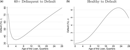
Transition probabilities
The graphs plot the transition probabilities (value-weighted) of loans that subsequently defaulted (i.e., the legal proceedings with the borrower are finalized). The plot on the left presents the default probabilities for loans that are 60 or more days late, whereas the one on the right presents those for loans that are paid on time or are less than 60 days late. We track loans from the quarter they become 60+ days late and plot the average loans that default conditional on their age at the quarter becoming delinquent (panel A). Similarly, we track loans from their origination quarter and plot the average loans that default conditional on the age of a loan (panel B). Both graphs are smoothed using fractional-polynomial approximation.
We estimate the recovery rates for each organizational level separately, as well as whether or not the loan is secured. The recovery data are available only for the first quarter of 2006. The estimated value-weighted recovery rate for individual secured loans is 40%, whereas for unsecured loans it is only 16%, reflecting the importance of the realization value of the collateral when seized in default (see Table 6). Our average estimated recovery rate is similar to the 25% provided by the Doing Business database from World Bank (2013). For robustness, we also check our results using three other recovery rates:24 25% as suggested by the Doing Business Database of the World Bank, a pessimistic 15%, and an optimistic 50%. Qualitatively, the results remain the same.
Recovery rates
| Mean | SE | Obs | ||
|---|---|---|---|---|
| (1) | (2) | (3) | ||
| Recovery rate |$\left(\delta\right)$| | Branch hierarchy: | |||
| Secured | Decentralized | 48.07 | 0.56 | 2,516 |
| Medium | 39.76 | 0.70 | 2,240 | |
| Centralized | 40.77 | 1.69 | 358 | |
| Unsecured | Decentralized | 30.07 | 0.46 | 4,420 |
| Medium | 23.47 | 0.46 | 3,699 | |
| Centralized | 23.28 | 1.02 | 595 |
The table reports the mean (Column 1) and the standard error (Column 2) of our estimated recovery rates, which are used in return on loan calculations. Additionally, Column 3 reports the number of observations used in calculating the rates. We report value-weighted recovery rates from the defaulted loans computed as the value recovered against the defaulted principal and interest due for both secured and unsecured loans. Because of data limitations, the recovery rates are calculated only for loans written off in the first quarter of 2006. Unfortunately, we do not have the data from other quarters.
Overall our results suggest that organizational hierarchy impedes information production and adversely affects not only the quality of loans but also their profitability. We find that the return on the same set of loans decreases after a branch becomes more hierarchical (Table 7). The value-weighted return on an individual loan decreases by 100 basis points (bps) (Column 2). Given that every quarter the bank earns 7.0% on every rupee lent (the value-weighted return), the 100-bps decline is equal to a 14% drop from the mean return. Similarly, for the equally weighted measure, the 70-bps fall in return (Column 1) is equivalent to a 10% slip in the branch’s performance. Further, the estimated results remain unchanged after controlling for local demand shocks through quarter-district fixed effects (Column 3) and do not have any pre-trend (Columns 5 and 6).25 Last, but not least, analogous to the delinquency result, we find a significant difference of 30 bps between value- and equally weighted measures (Column 4). This further supports the view that hierarchy leads to frictions in information production, suggesting that less hierarchical banks can allocate more money to profitable projects.
Return on loans
| ROL | ||||||
|---|---|---|---|---|---|---|
| Equally weighted | Value weighted | Value weighted | Difference (2)-(1) | Equally weighted | Value weighted | |
| (1) | (2) | (3) | (4) | (5) | (6) | |
| Branch level | −0.007*** | −0.010*** | −0.006*** | −0.003** | ||
| (0.002) | (0.002) | (0.002) | [0.011] | |||
| |${\rm Before}^{-2}$| | −0.001 | −0.000 | ||||
| (0.003) | (0.003) | |||||
| |${\rm Before}^{0}$| | −0.007** | −0.010*** | ||||
| (0.003) | (0.003) | |||||
| |${\rm After}^{2}$| | −0.003 | −0.010*** | ||||
| (0.003) | (0.002) | |||||
| |${\rm After}^{4+}$| | −0.008*** | −0.012*** | ||||
| (0.003) | (0.002) | |||||
| Observations | 54,079 | 54,079 | 54,079 | 54,079 | 54,079 | |
| Adj-|$R^{2}$| | 0.155 | 0.136 | 0.207 | 0.155 | 0.136 | |
| Branch FEs | Y | Y | Y | Y | Y | |
| Quarter FEs | Y | Y | N | Y | Y | |
| Quarter-district FEs | N | N | Y | N | N | |
This table reports the effect of organizational structure on the equally weighted and value-weighted return on loans (Columns 1, 2, and 3) and its dynamics (Columns 5 and 6) using specification (1). Column 3 reports the effect on value-weighted returns after controlling for local demand shocks through quarter-district fixed effects instead of quarterly fixed effects. Column 4 reports the difference between the estimated coefficients on equally and value-weighted returns. The unit of analysis is branch-quarter return on loans. First, we estimate the return for each loan, as defined in Equation (2). Then we aggregate the loan-level estimate at the branch-quarter level using equal or value weights. The variable Branch Level is a number between 1 and 3, where the lowest value (level 1) and the highest value (level 3) characterize the least hierarchical branches and the most hierarchical branches, respectively. |$\mbox{Before}^{-2}$| is a dummy variable that equals 1 (|$-1$|) if the branch was upgraded (downgraded) in one or two quarters. |$\mbox{Before}^{0}$| is a dummy variable that equals 1 (|$-1$|) if the branch was upgraded this quarter or one quarter ago. |$\mbox{After}^{2}$| is a dummy variable that equals 1 (|$-1$|) if the branch was upgraded (downgraded) two or three quarters ago. |$\mbox{After}^{4+}$| is a dummy variable that equals 1 (|$-1$|) if the branch was upgraded (downgraded) four quarters ago or more. Standard errors in parentheses are corrected for clustering at the branch level. p-values are reported in brackets. * significant at 10%; ** significant at 5%; and *** significant at 1%.
4.4 Standardization of loan contracts
In this section, we sharpen the evidence that organizational hierarchy leads to loss of information, by showing that contracts are more standardized in a hierarchical structure. To capture the information content in loans, we use a methodology similar in spirit to the procedure employed in Rajan et al. (2015) (similar to Cornell and Welch 1996; Cerqueiro et al. 2010). The intuition for this test can be understood using the following example. Consider two borrowers with identical hard information, but different soft information content. If a flatter organizational structure provides lenders with better information, then we should expect banks to discriminate between borrowers by giving more loans to the “good” types and less loans to the “bad” types. In the absence of such soft information, all borrowers with the same hard information would obtain similar loans. Thus, an increase in information would be captured by an increase in the dispersion of lending decisions.
4.4.1 Variance in quantity
In the first approach, we exploit two measures that have been used in the literature to capture information through variation in loan quantity: interquartile range and standard deviation of debt (see, for instance, Fisman et al. 2017). Both measures possess similar characteristics. The larger the amount of information, the larger the proxy. Using the difference-in-differences methodology defined in specification 1, qualitatively, both measures deliver the same result. Contracts become more standardized when a branch is converted to a more hierarchical unit (see Table 8). The interquartile range of debt (Column 1) and standard deviation of debt (Column 2) decrease by 12.3% and 9.5%, respectively. Furthermore, these effects remain unchanged from a qualitative point of view after absorbing all local shocks through quarter-district fixed effects (Columns 3 and 4). Lastly, in Columns 5 and 6, we investigate the dynamic effects and find no pre-trend. In fact, if anything, both pre-trend coefficients show the opposite signs. Moreover, all of the effects increase over time.
Contract standardization
| Dependent variable | |${\ln}\left(\mbox{IQR}_{b,q}\right)$| | |${\ln}\left(\sigma_{\mbox{loan}_{b,q}}\right)$| | “Quasi” R2 | |${\ln}\left(\mbox{IQR}_{b,q}\right)$| | |${\ln}\left(\sigma_{\mbox{loan}_{b,q}}\right)$| | Quasi R2 | |${\ln}\left(\mbox{IQR}_{b,q}\right)$| | |${\ln}\left(\sigma_{\mbox{loan}_{b,q}}\right)$| | “Quasi” R2 |
|---|---|---|---|---|---|---|---|---|---|
| (1) | (2) | (3) | (4) | (5) | (6) | (7) | (8) | (9) | |
| Branch level | −0.123*** | −0.095*** | −0.033*** | −0.112*** | −0.076*** | −0.022** | |||
| (0.026) | (0.021) | (0.008) | (0.029) | (0.023) | (0.009) | ||||
| |${\rm Before}^{-2}$| | −0.026 | 0.020 | −0.000 | ||||||
| (0.040) | (0.032) | (0.011) | |||||||
| |${\rm Before}^{0}$| | −0.135*** | −0.050 | −0.011 | ||||||
| (0.042) | (0.034) | (0.011) | |||||||
| |${\rm After}^{2}$| | −0.111*** | −0.102*** | −0.022* | ||||||
| (0.039) | (0.035) | (0.012) | |||||||
| |${\rm After}^{4+}$| | −0.145*** | −0.117*** | −0.046*** | ||||||
| (0.034) | (0.027) | (0.010) | |||||||
| Observations | 54,079 | 54,079 | 54,079 | 54,079 | 54,079 | 54,079 | 54,079 | 54,079 | 54,079 |
| Adj-|$R^{2}$| | 0.271 | 0.291 | 0.110 | 0.298 | 0.321 | 0.138 | 0.271 | 0.291 | 0.110 |
| Branch FEs | Y | Y | Y | Y | Y | Y | Y | Y | Y |
| Quarter FEs | Y | Y | Y | - | - | - | Y | Y | Y |
| Quarter-district FEs | N | N | N | Y | Y | Y | N | N | N |
The table reports the effect of organizational design on contract standardization: interquartile range of debt (Columns 1, 4, and 7), standard deviation of debt (Columns 2, 5, and 8), and the variation in the quantity conditional on other contractual characteristics: “quasi” R-squared (Columns 3, 6, and 9). “Quasi” R-squared captures the intensity of contract standardization at branch b, in quarter q. It is estimated as the standard deviation of the residuals obtained from the regression model defined in Equation (??). Columns 4 to 6 report the effect on contract standardization after controlling for local demand shocks through quarter-district fixed effects instead of quarterly fixed effects. The unit of analysis is a branch-quarter. The variable Branch level is a number between 1 and 3, where the lowest value (level 1) and the highest value (level 3) characterize the least hierarchical branches and the most hierarchical branches, respectively. |$\mbox{Before}^{-2}$| is a dummy variable that equals 1 (|$-1$|) if the branch was upgraded (downgraded) in one or two quarters. |$\mbox{Before}^{0}$| is a dummy variable that equals 1 (|$-1$|) if the branch was upgraded this quarter or one quarter ago. |$\mbox{After}^{2}$| is a dummy variable that equals 1 (|$-1$|) if the branch was upgraded (downgraded) two or three quarters ago. |$\mbox{After}^{4+}$| is a dummy variable that equals 1 (|$-1$|) if the branch was upgraded (downgraded) four quarters ago or more. The standard errors are reported in parentheses and clustered at the branch level. * significant at 10%; ** significant at 5%; and *** significant at 1%.
4.4.2 “Quasi” R-squared
The variance in the error term is an alternative way to look at the contract standardization. Because contractual terms are endogenous (jointly determined), some of the variation in the loan quantity might be explained by the variation in other contract terms. For example, a lender may increase the amount of a loan if a borrower pledges more collateral. Thus, one wishes to examine the variance in the loan quantity conditional on other contractual characteristics. The analysis of the error term permits that. The finding that the variance in the error term increases with a decrease in the organizational hierarchy suggests an information channel, controlling for all other contractual characteristics.
More specifically, to measure changes in the variance of quantity conditional on other contract terms, we run the following hedonic model:26
where |$i$| denotes a borrower, |$q$| denotes a quarter, and |$b$| is a branch. The dependent variable |$y_{biq}$| is the natural logarithm of the loan outstanding at the quarter of origination. The two fixed effects – |$\tau_{b}$| and |$\tau_{q}$| – capture the time invariant components of each branch and aggregate time-series shocks to all branches, respectively. |$X_{biq}$| is the vector of control variables. The vector of controls includes contract-specific characteristics, namely, maturity, value of the collateral, gender, and product group fixed effects.27 The residual |$\hat{\epsilon}_{biq}$| of this hedonic regression is the variation that is not explained by other contractual characteristics.28 In graph-form, we find that hierarchical branches are associated with more standardization. Figure 8 plots the kernel density functions of the residuals for decentralized and hierarchical branches.29 For the most hierarchical branches, the unexplained variation in loan quantity is more centered around the mean (zero) than for the more flatly organized branches, implying more contract standardization. As a final step, we calculate the standard deviation of these error terms and scale them by the variance of the dependent variable to generate a “quasi” R-squared. The lower the contract standardization and the more information, the lower the measured R-squared.
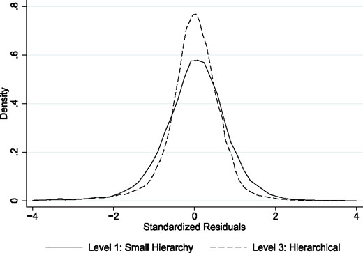
Cross-sectional variation
The graph plots the kernel density functions of standardized residuals (estimated by Equation 5) for loans falling within the approval limits of all branches. The graph is trimmed to show 98% of the sample.
Like for our results on variance in the quantity, we run our main DID specification for the “quasi” R-squared. Studying the same set of loans before and after the reorganization, we find that they become more standardized in a more hierarchical structure (Column 3 in Table 8). The estimated coefficient on the Branch level is negative and significant at 1%. In terms of economic magnitudes, the introduction of an additional managerial layer increases the contract standardization by roughly 5.3% when measured against the mean “quasi” R-squared. Furthermore, the results remain qualitatively the same after absorbing all local shocks through quarter-district fixed effects (Column 6).30 All in all, the findings on contract standardization support the view that a hierarchical structure leads to distortions in information production.
Figure 9 plots the dynamics of “quasi” R-squared around the branch reorganization that are estimated after controlling for branch and quarter fixed effects. The figure investigates issues of other contemporaneous events that might be driving the contract standardization and hence the change in the organizational design. As can be seen, there is no pre-trend and the results intensify over time. Column 9 of Table 8 reports the same result more formally. The estimated coefficient on the |${\rm Before}^{2}$| is economically small and statistically insignificant, meaning that there is no pre-trend in the data.
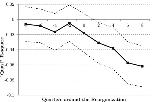
Dynamics plot: Contract standardization
The horizontal axis shows the time, in quarters, since the branch reorganization (0 represents the first two quarters of the reorganization). The vertical axis measures the contract standardization or “quasi” R-squared measured as the standard deviation of the residual estimated using Equation (5). The coefficients are estimated using Equation (3). The dashed lines indicate the 95% confidence interval.
All in all, our results suggest that loans become more standardized in more hierarchical structures; this finding is consistent with some recent research on contract standardization (Cornell and Welch 1996; Rajan et al. 2015). Taken together, our results in Section 4, provide support to this notion that an increase in organizational hierarchy adversely affects the allocation of bank credit. Banks not only reduce the quantity of loans disbursed but also those loans default more and are less profitable.
5. Other Results
5.1 Trade-off: Large loans
A rationale for upgrading a branch is to increase the maximum loan approval limit, that is, the loan size that can be approved internally in a given branch. After upgrading a branch, the organizational distance between the borrower and the decision maker increases for small loans. But the opposite is true for the loans that were above the approval limit of the branch and had to be approved externally before the upgrade.31 If the information argument is true for small loans, it is likely to also hold for the larger ones. Thus, large loans should benefit from the upgrade, as the manager can now decide about the loans internally.
We find an improvement in the lending outcomes on large loans (see Table 9). This finding provides additional support for our results on small loans. First, to capture the effect on the total debt granted, we use |$\ln\left(1+Debt\right)$| as the dependent variable (Column 1). Second, the effect on the large loan extensive margin, that is, the probability of a large loan being granted, is captured by a linear probability model (Column 2). Third, as the average number of “large loans” per branch-quarter is 1.4, computing the second moment of the residual, our measure for contract standardization, becomes challenging. Therefore, we use the mean absolute value of the residual estimated in specification 5 (Column 3). The properties of this measure are similar to the main proxies of contract standardization “quasi” R-squared. The less standardized is a contract, the greater the mean absolute value.32
Effect of organizational design on large loans, eligible for approval internally
| |$\ln\left(1+\mbox{value}_{b,q}\right)$| | |${\rm 1}\kern-0.24em{\rm I}_{\mbox{#loans}_{b,q}>0}$| | Residual | |$\ln\left(1+\mbox{value}_{b,q}\right)$| | |${\rm 1}\kern-0.24em{\rm I}_{\mbox{#loans}_{b,q}>0}$| | Residual | |
|---|---|---|---|---|---|---|
| (1) | (2) | (3) | (4) | (5) | (6) | |
| Branch level | 0.509*** | 0.033*** | 0.016*** | |||
| (0.150) | (0.011) | (0.004) | ||||
| |${\rm Before}^{-2}$| | 0.305 | 0.019 | 0.005 | |||
| (0.205) | (0.015) | (0.005) | ||||
| |${\rm Before}^{0}$| | 0.617*** | 0.041*** | 0.013** | |||
| (0.210) | (0.015) | (0.006) | ||||
| |${\rm After}^{2}$| | 0.530** | 0.034** | 0.013** | |||
| (0.221) | (0.016) | (0.005) | ||||
| |${\rm After}^{4+}$| | 0.565*** | 0.036** | 0.019*** | |||
| (0.202) | (0.014) | (0.005) | ||||
| Observations | 54,079 | 54,079 | 54,079 | 54,079 | 54,079 | 54,079 |
| |${\rm Adj}-R^{2}$| | 0.324 | 0.309 | 0.253 | 0.324 | 0.309 | 0.253 |
| Quarter FE | Y | Y | Y | Y | Y | Y |
| Branch FEs | Y | Y | Y | Y | Y | Y |
This table reports the effect of organizational design on loans that had to be approved externally (e.g., regional office) before the change, but can be approved internally since the increase in the approval limit of the branch. We report the estimated effect on log debt amount (Columns 1 and 4), the probability of receiving any credit (Columns 2 and 5), and contract standardization (Columns 3 and 6) using specification (1). The measure of contract standardization is the mean absolute value of the residual, estimated by Equation (5). The unit of analysis is a branch-quarter. The variable Branch level is a number between 1 and 3, where the lowest value (level 1) and the highest value (level 3) characterize the least hierarchical branches and the most hierarchical branches, respectively. |$\mbox{Before}^{-2}$| is a dummy variable that equals 1 (|$-1$|) if the branch was upgraded (downgraded) in one or two quarters. |$\mbox{Before}^{0}$| is a dummy variable that equals 1 (|$-1$|) if the branch was upgraded (downgraded) this quarter or one quarter ago. |$\mbox{After}^{2}$| is a dummy variable that equals 1 (|$-1$|) if the branch was upgraded (downgraded) two or three quarters ago. |$\mbox{After}^{4+}$| is a dummy variable that equals 1 (|$-1$|) if the branch was upgraded (downgraded) four quarters ago or more. The standard errors are reported in parentheses and clustered at the branch level. * significant at 10%; ** significant at 5%; and *** significant at 1%.
The estimated coefficients on the Branch Level are positive and significant across all three specifications. The estimates imply that lending of large loans increases when the approval of these “large” loans is carried out internally (Column 1), and the probability of issuing a large loan increases by 3.3 percentage points (Column 2). The latter result is equivalent to a 21% increase in the average probability of issuing a large loan. Contracts are also less standardized (Column 3). To address the reverse causality, we also show the dynamic effects. None of the estimated effects have a pre-trend.
Although small loans suffer from the hierarchy, the very large borrowers, who, in terms of physical distance, are closer to the decision maker after a branch is centralized, benefit from the proximity. Thus, while a branch might be losing on the small loans, it could recover the loss through gains from the large loans. Therefore, we examine how organizational hierarchy affects the combined retail portfolio including both small and large loans.
We find that when a branch is upgraded, the gains on large loans are not sufficient to cover the losses that a branch makes on the small loans. In the combined retail portfolio, the default rates increase and returns decrease (Columns 4 and 5 in Table 10), while the lending volume remains unchanged (Column 6). We also find that the loan contracts are more standardized (Columns 1 through 3). Thus, the overall effect on the retail portfolio remains negative.
Combined retail portfolio
| “Quasi” R2 | |$\ln\left(\sigma_{\mbox{loan}_{b,q}}\right)$| | |$\ln\left(\mbox{IQR}_{b,q}\right)$| | VW default | VW ROL | |$\ln\left(\mbox{new ind.}\right.$| | |
|---|---|---|---|---|---|---|
| |$\left.\mbox{debt}_{b,q}\right)$| | ||||||
| (1) | (2) | (3) | (4) | (5) | (6) | |
| Branch level | −0.033*** | −0.043* | −0.092*** | 0.013*** | −0.004** | −0.038 |
| (0.008) | (0.023) | (0.027) | (0.003) | (0.002) | (0.030) | |
| Obs | 54,079 | 54,079 | 54,067 | 54,079 | 54,079 | 54,079 |
| Adj-|$R^{2}$| | 0.107 | 0.408 | 0.350 | 0.187 | 0.157 | 0.469 |
| Branch FEs | Y | Y | Y | Y | Y | Y |
| Quarter FEs | Y | Y | Y | Y | Y | Y |
In this table, we report the effect of the organizational hierarchy for the combined retail portfolio (i.e., it includes both small and large loans). We report the effect on the contract standardization (“quasi” R-squared), standard deviation of debt, interquartile range of debt, value-weighted defaults and return on loans, and total new lending to retail borrowers in Columns 1 through 6, respectively. The unit of analysis is a branch-quarter. The measure of contract standardization is estimated as the standard deviation of the residuals obtained from the regression model defined in Equation (5). The defaults are measured as whether a loan is over 60 days late 1-year forward. The return on loans is measured as defined in Equation (2). The variable Branch Level is a number between 1 and 3, where the lowest value (level 1) and the highest value (level 3) characterize the least hierarchical branches and the most hierarchical branches, respectively. The standard errors are reported in parentheses and clustered at the branch level. * significant at 10%; ** significant at 5%; and *** significant at 1%.
Although better performance on larger loans does not offset the inferior performance on smaller loans, this is a trade-off worth highlighting. It is important to note that we measure costs at the branch level. To understand the overall effect of organizational hierarchy, one has to evaluate the performance of the bank. Upgrading a branch frees up resources at regional, zonal, or central offices, because large loans are approved internally afterward. As a result, regional- or higher- level offices are less overburdened with tasks from local branches, making them more effective in other bank-level assignments. For instance, these offices can focus on business development, marketing campaigns, risk management, and other activities that affect the overall performance of the bank. The data are consistent with this. During our sample, the profitability of the bank increased, suggesting that the aggregate effect of hierarchization was positive. Furthermore, the bank opened branches in 43 previously unbanked districts, thereby accessing new markets. With that in mind, we refrain from making any claims on the overall profitability of the bank, because we do not have a control group for the bank-level analysis.
5.2 Hierarchy and corruption
Full delegation in the presence of corruption is a double-edged sword (Tirole 1986; Banerjee et al. 2013). On the one hand, if the private benefits of an agent are aligned with those of the principal, delegation may be a good idea, as it creates an extra incentive to perform the task. For instance, Bandiera et al. (2009) document that giving more discretion to bureaucrats in Italian public procurement may lead to budget savings, even though it allows the bureaucrat to pocket some of the money. On the other hand, if an agent’s private benefits are not aligned with the profit-maximizing behavior of the principal, it may be worthwhile maintaining control over the employees. Essentially, the nature of corruption determines the optimal level of discretion.
To understand how organizational hierarchy interacts with rent-extraction, we compare the effects in more corrupt states to those in the less corrupt ones. We proxy for corruption with two measures. The first one focuses on branches in the so-called “BIMARU states,” (Bihar, Madhya Pradesh, Rajasthan, and Uttar Pradesh) which have been singled out for corruption (see, e.g., Kumar, 2007).33 The second measure is the corruption index provided by Transparency International. The index is particularly useful for our study, because it examines corruption in banking services. It measures the fraction of respondents who actually paid a bribe for obtaining these services. The study points out that the majority of these bribes were paid to secure a loan. The size of such a bribe ranges between 5% and 10% of the notional value.34 The corruption measure is reported at the state level and ranges from 1.2% in West Bengal to 39.2% in Bihar.
Both measures indicate that the negative effects of organizational hierarchy are mitigated in more corrupt areas (see Table 11). These findings are in line with the view that greater delegation reduces information frictions, while simultaneously enabling rent extraction. However, if the decision-making were centralized in the corrupt branches, the benefits of limiting corruption would attenuate the loss of information. The point estimates suggest that the effect of hierarchy disappears or becomes positive in very corrupt areas (corruption index of 39.2%). This highlights the gains of having organizational hierarchy in areas prone to more corruption.
Organizational hierarchy and corruption
| “Quasi” R2 | VW ROL | VW default | “Quasi” R2 | VW ROL | VW default | |
|---|---|---|---|---|---|---|
| (1) | (2) | (3) | (4) | (5) | (6) | |
| Branch level | −0.046*** | −0.016*** | 0.020*** | −0.063*** | −0.024*** | 0.028*** |
| (0.009) | (0.002) | (0.003) | (0.013) | (0.004) | (0.005) | |
| Branch level x BIMARU | 0.043** | 0.019*** | −0.021*** | |||
| (0.018) | (0.005) | (0.006) | ||||
| Branch level x | 0.190** | 0.091*** | -0.091*** | |||
| % Experience corruption | (0.080) | (0.028) | (0.034) | |||
| Obs | 54,079 | 54,079 | 54,079 | 53,475 | 53,475 | 53,475 |
| Adj-|$R^{2}$| | 0.110 | 0.137 | 0.183 | 0.110 | 0.136 | 0.184 |
| Branch FEs | Y | Y | Y | Y | Y | Y |
| Quarter FEs | Y | Y | Y | Y | Y | Y |
The table reports the effect of organizational design depending on the severity of corruption in the area. We report the estimated effect on the measure of contract standardization (Columns 1 and 4), value-weighted return on loans (Columns 2 and 5) and default (Columns 3 and 6). The unit of analysis is a branch-quarter. The variable Branch level is a number between 1 and 3, where the lowest value (level 1) and the highest value (level 3) characterize the least hierarchical branches and the most hierarchical branches, respectively. BIMARU is a dummy variable equal to one if the branch is located in the states of Bihar, Madhya Pradesh, Rajasthan, and Uttar Pradesh, which have been singled out for corruption and dysfunction (columns 1 through 3). % Experience Corruption, provided by Transparency International, measures the fraction of people who had to pay a bribe to receive banking services in any given state. Please note that the number of observations in Columns 4 through 6 is slightly lower because the study by Transparency International does not report the results for three states: Chandigarh, Dadra and Nagar, Haveli Daman and Diu. The standard errors are reported in parentheses and clustered at the branch level. * significant at 10%; ** significant at 5%; and *** significant at 1%.
5.3 Preexisting borrowers
We now turn to evaluating how organizational hierarchy affects borrowers who have an existing credit record with the bank. This comparison is useful, because the bank may have generated information about these borrowers during the relationship. Thus, it is plausible that the negative effect of the branch hierarchization is weaker. To examine this, we repeat our difference-in-differences test on the sample of all repeat borrowers. We find that the results are somewhat weaker (Table 12). Overall, the weaker effect on existing borrowers is consistent with the view that some of the information generated in the due course of a relationship. Thus, the loss of information due to organizational hierarchy is not as large.
Repeat borrowers
| “Quasi” R2 | VW ROL | VW defaults | |$\ln\left(\mbox{new ind.}\right.$| | |
|---|---|---|---|---|
| |$\left.\mbox{debt}_{b,q}\right)$| | ||||
| (1) | (2) | (3) | (4) | |
| Branch level | −0.027** | −0.014** | 0.006 | 0.031 |
| (0.013) | (0.006) | (0.006) | (0.049) | |
| Observations | 20,988 | 20,988 | 20,988 | 20,988 |
| Adj-|$R^{2}$| | 0.087 | 0.115 | 0.140 | 0.315 |
| Branch FEs | Y | Y | Y | Y |
| Quarter FEs | Y | Y | Y | Y |
The table reports results on all repeat borrowers. We report the estimated effect on the measure of contract standardization (“quasi” R-squared, Columns 1), value-weighted return on loans (Column 2) and default (Column 3), and total new lending to small individual borrowers (Column 4). The unit of analysis is a branch-quarter. The variable Branch Level is a number between 1 and 3, where the lowest value (level 1) and the highest value (level 3) characterize the least hierarchical branches and the most hierarchical branches, respectively. The standard errors are reported in parentheses and clustered at the branch level. * significant at 10%; ** significant at 5%; and *** significant at 1%.
5.4 Upgrades versus downgrades
The difference-in-differences empirical strategy employed so far identifies the effect of hierarchy on lending. It assumes that upgrades and downgrades are symmetric. Here, we examine whether the treatment effect is symmetric.
On examining upgrades and downgrades separately, we find asymmetric effects (Table 13).35 While the upgrade results in a lowering of both the quantity and quality of credit, the reverse is not true for the downgrade. A plausible explanation for these effects deals with the differential labor adjustment following an upgrade vis-à-vis a downgrade. When a branch is upgraded, it gains a senior-level manager along with some other lower-level support staff to cope with the increased scale of business. This relaxes the resource constraints facing the branch prior to the upgrade and generates immediate results. In the case of the downgrade, however, it takes time to reallocate the existing staff to other branches, as labor laws make it difficult to lay off an employee. Furthermore, there is a view that banks are overstaffed, so there is no obvious place they can be relocated. Also, moving them around is costly, as the bank has to pay relocation costs, which are quite substantial.36 Thus, when the branch is upgraded, it obtains the resources relatively quickly. This adjustment, however, is slower in the case of a downgrade, because the bank needs to find an appropriate place where they can justify the relocation in terms of costs. Consistent with this, when the downgrade and upgrade happen in the same district, this adjustment is fast and we find that downgrades generate symmetric effects. The results are reported in Table 14.
Upgrades versus downgrades
| “Quasi” R2 | |$\ln\left(\mbox{IQR}_{b,q}\right)$| | |$\ln\left(\sigma_{\mbox{loan}_{b,q}}\right)$| | VW ROL | VW defaults | |$\ln\left(\mbox{new ind.}\right.$| | |||||||
|---|---|---|---|---|---|---|---|---|---|---|---|---|
| |$\left.\mbox{debt}_{b,q}\right)$| | ||||||||||||
| (1) | (2) | (3) | (4) | (5) | (6) | |||||||
| A. Upgrades | ||||||||||||
| Branch level | −0.047*** | −0.133*** | −0.119*** | −0.011*** | 0.015*** | −0.113*** | ||||||
| (0.009) | (0.031) | (0.025) | (0.002) | (0.003) | (0.036) | |||||||
| Adj-|$R^{2}$| | 0.110 | 0.269 | 0.291 | 0.136 | 0.182 | 0.395 | ||||||
| B. Downgrades | ||||||||||||
| Branch level | 0.018 | −0.078 | −0.003 | −0.005 | 0.008 | −0.039 | ||||||
| (0.018) | (0.055) | (0.047) | (0.005) | (0.007) | (0.054) | |||||||
| Adj-|$R^{2}$| | 0.109 | 0.264 | 0.291 | 0.137 | 0.186 | 0.406 | ||||||
| Branch FEs | Y | Y | Y | Y | Y | Y | ||||||
| Quarter FEs | Y | Y | Y | Y | Y | Y | ||||||
The table reports the results using a sample of all branch upgrades (panel A) and downgrades (panel B). The control group are all branches that did not change their organizational design. We report the estimated effect on the three measures of contract standardization (Columns 1 to 3), value-weighted return on loans (Column 4) and default (Column 5), and total new lending to small individual borrowers (Column 6). The unit of analysis is a branch-quarter. The variable Branch Level is a number between 1 and 3, where the lowest value (level 1) and the highest value (level 3) characterize the least hierarchical branches and the most hierarchical branches, respectively. The standard errors are reported in parentheses and clustered at the branch level. * significant at 10%; ** significant at 5%; and *** significant at 1%.
Downgrades with a nearby upgrade
| “Quasi” R2 | |$\ln\left(\mbox{IQR}_{b,q}\right)$| | |$\ln\left(\sigma_{\mbox{loan}_{b,q}}\right)$| | VW ROL | VW defaults | |$\ln\left(\mbox{new ind.}\right.$| | |
|---|---|---|---|---|---|---|
| |$\left.\mbox{debt}_{b,q}\right)$| | ||||||
| (1) | (2) | (3) | (4) | (5) | (6) | |
| Branch level | 0.034 | −0.257*** | −0.145* | −0.013* | 0.019* | −0.144* |
| (0.023) | (0.099) | (0.077) | (0.007) | (0.011) | (0.085) | |
| |${\rm Adj}-R^{2}$| | 0.110 | 0.262 | 0.290 | 0.138 | 0.186 | 0.405 |
| Branch FEs | Y | Y | Y | Y | Y | Y |
| Quarter FEs | Y | Y | Y | Y | Y | Y |
The table reports the results using a sample of branch downgrades that are accompanied with an upgrade of another branch in the same district within a year. The control group consists of all branches that did not change their organizational design. We report the estimated effect on the three measures of contract standardization (Columns 1 to 3), value-weighted return on loans (Column 4) and default (Column 5), and total new lending to small individual borrowers (Column 6). The unit of analysis is a branch-quarter. The variable Branch level is a number between 1 and 3, where the lowest value (level 1) and the highest value (level 3) characterize the least hierarchical branches and the most hierarchical branches, respectively. The standard errors are reported in parentheses and clustered at the branch level. * significant at 10%; ** significant at 5%; and *** significant at 1%.
5.5 Nonlinear effects
Next, we examine whether reorganization from 1 to 2 generates similar effects compared to a reorganization from 2 to 3. Our main specification treats these as equal. Here, we augment our main specification by adding an interaction of branch level and a dummy variable of whether the reorganization was between levels 1 and 2 or 2 and 3. We find some convexities in the costs that are associated with organizational hierarchy. The effects are stronger for changes from 2 to 3 as opposed from 1 to 2 (see Table 15). This finding is consistent with the Williamsonian view on the dis-economies of scale in organizations (Williamson 1967; Williamson 1988).
Nonlinear effects of hierarchy
| “Quasi” R2 | |$\ln\left(\mbox{IQR}_{b,q}\right)$| | |$\ln\left(\sigma_{\mbox{loan}_{b,q}}\right)$| | VW ROL | VW defaults | |$\ln\left(\mbox{new ind.}\right.$| | |
|---|---|---|---|---|---|---|
| |$\left.\mbox{debt}_{b,q}\right)$| | ||||||
| (1) | (2) | (3) | (4) | (5) | (6) | |
| Branch level | −0.020** | −0.125*** | −0.075*** | −0.008*** | 0.012*** | −0.059* |
| (0.009) | (0.030) | (0.025) | (0.002) | (0.003) | (0.034) | |
| Branch level x | −0.052*** | 0.007 | −0.083* | −0.009** | 0.008 | −0.160** |
| Change 2-3 | ||||||
| (0.018) | (0.058) | (0.044) | (0.004) | (0.005) | (0.071) | |
| Observations | 54,079 | 54,079 | 54,079 | 54,079 | 54,079 | 54,079 |
| Adj-|$R^{2}$| | 0.110 | 0.270 | 0.291 | 0.136 | 0.183 | 0.396 |
| Branch FEs | Y | Y | Y | Y | Y | Y |
| Quarter FEs | Y | Y | Y | Y | Y | Y |
The table reports the additional effect of changing hierarchy from 2 to 3 (or 3 to 2). The dummy variable Change 2-3 equals 1 if the organizational change is from 2 to 3 or 3 to 2 and zero otherwise. We report the estimated effect on the three measures of contract standardization (Columns 1 to 3), value-weighted return on loans (Column 4) and default (Column 5), and total new lending to small individual borrowers (Column 6). The unit of analysis is a branch-quarter. The variable Branch Level is a number between 1 and 3, where the lowest value (level 1) and the highest value (level 3) characterize the least hierarchical branches and the most hierarchical branches, respectively. The standard errors are reported in parentheses and clustered at the branch level. * significant at 10%; ** significant at 5%; and *** significant at 1%.
6. Robustness
We have so far shown that a change in organizational design affects a bank’s ability to produce information on loans and has implications for capital allocation decisions by banks. This section addresses a few more items that could potentially confound our inference.
6.1 New officer effect
A change in organizational design also brings in a new official as the head of the branch. If the branch is upgraded to a higher level, it brings in a more experienced and senior official to head the branch. One would expect that the presence of an experienced official should improve the credit allocation decision in the bank because the loan officer, approving loans earlier, now has access to a more knowledgeable advisor. It should be noted that such an effect, if present, would lead to increased information and lower defaults on loans, thus biasing against finding the result that we have identified in the paper.
In a similar vein, one could argue that the arrival of a new branch manager leads to a temporary loss of information and thus generates both poor performance of loans and higher standardization (a new officer tends to overrely on hard information). This story may seem plausible, but it is not supported by our data. First, such an effect should also be present, and perhaps to a higher degree, when officers are rotated without the change in organizational design. We exploit an internal rotation policy of branch managers and do not find this to be the case (see Table 16).37 Second, we do not find the effect to be transient; that is, the effects do not reverse once the officer is comfortable in the new system.
Manager rotation
| “Quasi” R2 | VW ROL | VW defaults | |$\ln\left(\overline{\mbox{loan}}_{b,q}\right)$| | |$\ln\left(\mbox{new ind.}\right.$| | |$\ln\left(\sigma_{\mbox{loan}_{b,q}}\right)$| | |$\ln\left(\mbox{IQR}_{b,q}\right)$| | |
|---|---|---|---|---|---|---|---|
| |$\left.\mbox{debt}_{b,q}\right)$| | |||||||
| (1) | (2) | (3) | (4) | (5) | (6) | (7) | |
| Change | −0.012 | −0.002 | −0.001 | 0.014 | −0.012 | 0.029 | 0.038 |
| (0.011) | (0.003) | (0.004) | (0.023) | (0.041) | (0.031) | (0.038) | |
| Obs | 33,684 | 33,684 | 33,684 | 33,684 | 33,684 | 33,684 | 33,684 |
| Adj-|$R^{2}$| | 0.135 | 0.131 | 0.188 | 0.454 | 0.395 | 0.328 | 0.297 |
| Branch FEs | Y | Y | Y | Y | Y | Y | Y |
| Quarter FEs | Y | Y | Y | Y | Y | Y | Y |
The table reports the results of manager rotation when the organizational design remains unchanged. We show the estimated effects on the contract standardization (“quasi” R-squared, Column 1), the value weighted return on loans (Column 2) and defaults (Column 3), log average loan (Column 4), log total new individual lending (Column 5), standard deviation of debt (Column 6), and the interquartile range of debt (Column 7). The unit of analysis is a branch-quarter. The variable Change is a dummy variable equal to one if the manager changed at the branch b, in quarter q, and zero otherwise. The measure of contract standardization is estimated as the standard deviation of the residuals obtained from the regression model defined in Equation (5). The defaults are measured as whether a loan is over 60 days late 1-year forward. The standard errors are reported in parentheses and clustered at the branch level. * significant at 10%; ** significant at 5%; and *** significant at 1%.
6.2 Manipulation
As noted above, the reorganization of a branch entails a change in the loan approval limit. This change in the cutoff point may alter the composition of borrowers around the threshold. This can be demonstrated by the following situation. An individual with no credit history or adverse credit history requests a loan of 550,000 rupees from a manager whose approval limit is only 500,000 rupees. Even though, after a thorough investigation, the manager knows that the borrower is of the good type, the very nature of the information makes it extremely difficult to transmit it to the regional office. Hence, forwarding the application further would clearly lead to a rejection. Anticipating this, the manager may instead offer the client a loan of 500,000 rupees that falls within his approval limit. If such terms are acceptable to both parties, a loan is granted. However, in the period after upgradation, the branch manager who is heading this branch does not face this dilemma (if the approval limit is above 550,000 rupees) as he can approve this loan within the branch. He would then simply approve the 550,000 rupee loan. Thus, manipulation of the loan amount may change the composition of borrowers around the threshold.
Additional tests show that this does not affect our results. We begin by plotting the Epanechnikov kernel density functions around the normalized cutoff for pre- and post-treatment periods. As can be seen in Figure 10, both distributions are statistically the same around the cutoff point and the Kolmogorov-Smirnov test for the equality of the distributions cannot be rejected at the 1% level. In other words, we find no evidence of any bunching around the threshold.38 Next, we disregard loans that are within a 20% window around the cutoff39 and reestimate our specification. Our results remain virtually the same with the lower approval limit (Table 17). Finally, as already noted, the smallest common cutoff is binding only for a subset of bank branches (roughly one-sixth of branches). Excluding those branches leaves our results qualitatively unchanged. In sum, all three tests allay all concerns of manipulation around the cutoff.
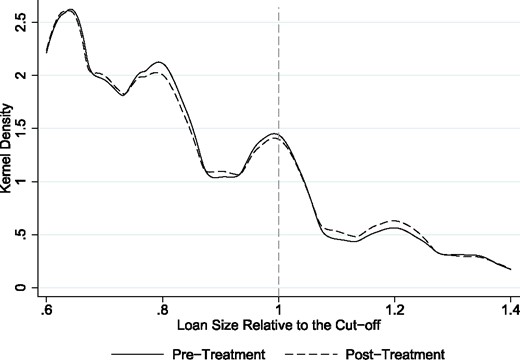
Distribution around the approval threshold
The graph plots kernel density functions of loans around the threshold value for pre- and post-treatment periods. The threshold is normalized to equal 1. We show the frequency of all loans that fall within the 40% window around the threshold value. The values to the right of 1.00 are above the threshold, and the values to the left are below it.
Loan size manipulation around the approval limit
| VW defaults | VW ROL | “Quasi” R2 | ||
|---|---|---|---|---|
| (1) | (2) | (3) | (4) | |
| Branch level | 0.013*** | −0.008*** | −0.035*** | |
| (0.003) | (0.004) | (0.008) | ||
| |${\rm Before}^{-2}$| | 0.006 | |||
| (0.011) | ||||
| |${\rm Before}^{0}$| | −0.009 | |||
| (0.012) | ||||
| |${\rm After}^{2}$| | −0.022* | |||
| (0.013) | ||||
| |${\rm After}^{4+}$| | −0.047*** | |||
| (0.010) | ||||
| Observations | 54,079 | 54,079 | 54,079 | 54,079 |
| Adj-|$R^{2}$| | 0.18 | 0.13 | 0.11 | 0.11 |
| Branch FEs | Y | Y | Y | Y |
| Quarter FEs | Y | Y | Y | Y |
In this table, we report the effect of the organizational hierarchy for the loans well below the loan approval limit of the head of the branch. We redefine the approval limit as 80% of the true threshold. We report the effect on the value-weighted defaults (Column 1) and return on loans (Column 2), and the contract standardization (“quasi” R-squared, Columns 3 and 4). The unit of analysis is a branch-quarter. The measure of contract standardization is estimated as the standard deviation of the residuals obtained from the regression model defined in Equation (5). The defaults are measured as whether a loan is over 60 days late 1-year forward. The return on loans is measured like in Equation (2). The variable Branch Level is a number between 1 and 3, where the lowest value (level 1) and the highest value (level 3) characterize the least hierarchical branches and the most hierarchical branches, respectively. |$\mbox{Before}^{-2}$| is a dummy variable that equals 1 (|$-1$|) if the branch was upgraded (downgraded) in one or two quarters. |$\mbox{Before}^{0}$| is a dummy variable that equals 1 (|$-1$|) if the branch was upgraded this quarter or one quarter ago. |$\mbox{After}^{2}$| is a dummy variable that equals 1 (|$-1$|) if the branch was upgraded (downgraded) two or three quarters ago. |$\mbox{After}^{4+}$| is a dummy variable that equals 1 (|$-1$|) if the branch was upgraded (downgraded) four quarters ago or more. The standard errors are reported in parentheses and clustered at the branch level. * significant at 10%; ** significant at 5%; and *** significant at 1%.
6.3 Borrower switching
We have extended our analysis to account for the possibility that borrowers could be switching (1) across branches within the bank or (2) to branches of other banks. To account for switching, we evaluate geographic areas with few outside options, that is, areas with no other bank branch of this or any other bank in close proximity. We obtain data from the bank on branch offices that are the sole banking services provider within an 8- to 10-kilometer radius (panel A of Table 18). For robustness, we examine branches that are the sole bank branch within a banking area, as defined by the Reserve Bank of India (panel B of Table 18).40 Using both measures, we find similar effects in these isolated areas.41 Thus, it is unlikely that our results are driven by borrower switching. The effects are very similar to the main specification, except for the result on total lending.
Lead bank
| “Quasi” R2 | |$\ln\left(\mbox{IQR}_{b,q}\right)$| | |$\ln\left(\sigma_{\mbox{loan}_{b,q}}\right)$| | VW ROL | VW defaults | |$\ln\left(\mbox{new ind.}\right.$| | |
|---|---|---|---|---|---|---|
| |$\left.\mbox{debt}_{b,q}\right)$| | ||||||
| (1) | (2) | (3) | (4) | (5) | (6) | |
| A. Single branch within 8–10 km | ||||||
| Branch level | −0.030** | −0.136*** | −0.058* | −0.008*** | 0.011*** | 0.003 |
| (0.015) | (0.044) | (0.035) | (0.003) | (0.004) | (0.047) | |
| Observations | 24,111 | 24,111 | 24,111 | 24,111 | 24,111 | 24,111 |
| Adj-|$R^{2}$| | 0.110 | 0.199 | 0.232 | 0.122 | 0.150 | 0.412 |
| B. Reserve Bank of India measure | ||||||
| Branch level | −0.018 | −0.173*** | −0.091** | −0.008 | 0.013** | −0.065 |
| (0.018) | (0.048) | (0.045) | (0.005) | (0.006) | (0.058) | |
| Observations | 24,923 | 24,923 | 24,923 | 24,923 | 24,923 | 24,923 |
| |$\mbox{Adj}-R^{2}$| | 0.122 | 0.200 | 0.250 | 0.137 | 0.190 | 0.407 |
| Quarter FEs | Y | Y | Y | Y | Y | Y |
| Branch FEs | Y | Y | Y | Y | Y | Y |
The table reports results for branches that are the only branch in an area: (1) 8- to 10-kilometer radius as provided by the Bank (panel A), (2) banking area, as defined by the Reserve Bank of India (panel B). We report the estimated effect on the three measures of contract standardization (Columns 1 to 3), value-weighted return on loans (Column 4) and default (Column 5), and total new lending to small individual borrowers (Column 6). The unit of analysis is a branch-quarter. The variable Branch Level is a number between 1 and 3, where the lowest value (level 1) and the highest value (level 3) characterize the least hierarchical branches and the most hierarchical branches, respectively. The standard errors are reported in parentheses and clustered at the branch level. * significant at 10%; ** significant at 5%; and *** significant at 1%.
7. Discussion and Conclusion
A large literature in financial intermediation delegates the role of screening and monitoring to banks. In accordance with these theories, delegation is efficient, because it reduces duplication in monitoring costs and free-riding problems that are associated with multiple creditors. But for a bank to deliver on these tasks, it must have the correct organizational design in place.
Several theories postulate a link between organizational hierarchy and lending, but empirical work has lagged behind. In this paper, we use a quasi-natural experiment research design to investigate this question and find that an increase in hierarchy adversely affects lending. We find that hierarchization of a branch increases the delinquency rate by 30% and decreases the return on loans by 14%. Furthermore, it leads to standardization of loan contracts. Overall, our findings suggest that a hierarchical organizational structure distorts production and communication of information.
A few points are worth highlighting. First, our study documents trade-offs associated with the organizational hierarchy at a branch level, but it is silent on overall bank profitability. It is very likely that the bank overall benefits from the organizational restructuring, as the bank’s profits have increased during our sample. Upgrading a branch, for example, frees up resources at regional- and higher-level offices. These offices can direct their efforts toward business development and other bank-level assignments. For instance, this bank expanded its reach and opened up new branches in several previously unbanked areas (in total 43 previously unbanked districts during our sample). Because we lack a control group, we refrain from making any causal claims about overall bank profitability. Furthermore, our analysis suggests that the negative effects of organizational hierarchy are mitigated in more corrupt areas.
Second, this paper identifies the effect of hierarchy on information production, but it does so in a setting in which incentive contracts are fixed across different branches. This is ideal from an identification point of view, but it leaves the following questions unanswered: can one overcome the problem of hierarchies with well-designed incentive contracts, or are there limits to delegation in these branches? These are important questions for future research.
Third, our paper also shows that large organizations mitigate the problem of transmitting information by creating within-firm suborganizations. Although the bank is very hierarchical with many layers of managers, it creates branch offices and commits to credibly delegate decision-making power to those offices. In line with Stein’s (2002) view that more hierarchical firms tend to base their decisions on hard information, this result shows that banks are able to mitigate this challenge internally.
Fourth and finally, our results may have important implications for economic inequality. The current trend toward more globalized and hierarchical banks raise natural concerns that low-income (also ‘soft’ information) borrowers may be left behind. If so, such a shift may aggravate inequality in society. This may not be an issue in a frictionless world, where new intermediaries would enter to fill this gap. But recent events give us reason to be suspicious of this benign “Coasian” view of the world. In reality, markets may be slow to adapt, and low-income borrowers may be thrown into a vicious poverty trap. It is useful to recall the recent case of former Federal Reserve Bank Chairman, Ben Bernanke, who failed to refinance his house, because loan pricing models overestimated his credit risk after his job switch to Princeton University.42 This example underscores the dangers of increased reliance on hard information. Ultimately, how the organization of finance affects inequality is an important and interesting question for future research.
We thank Andres Almazan, Tobias Berg, Joao Cocco, Julian Franks, Oliver Hart, Robert Hauswald, Maggie Hu, Jose Liberti, Wenlan Qian, Oleg Rubanov, Rui Silva, Denis Sosyura, and Philip Strahan and seminar participants at the 9th NY Fed/NYU Stern Conference on Financial Intermediation, the 3rd MoFiR workshop, the 6th Financial Stability Conference, the 11th Annual Conference on Corporate Finance, ISNIE (Duke), CICF (China), London Business School, the Summer Research Conference 2014 (ISB), the Summer Real Estate Symposium (Monterey), University of Nottingham, University of Surrey, University of Washington (Foster), UBC, WFA (Monterey), and AEA (Boston) for their comments. Supplementary data can be found on The Review of Financial Studies web site.
Footnotes
Some notable contributions include Berger et al. (2005), Liberti and Mian (2009), Canales and Nanda (2012), and Liberti et al. (2015, 2017).
It should be noted that all branches that have the same level are standardized with a nearly identical organizational design. Furthermore, the level of the branch (levels 1, 2, and 3) is directly linked to the seniority of the branch manager presiding it. Put differently, the approval limit of a branch comes from the approval limit of the branch manager.
If a borrower requests a loan above a branch office’s limit, the request will be referred to (1) a regional office, (2) a zonal office, or (3) the central office. A regional office’s approval limits are above those of any branch in the region; a zonal office’s are above all regional offices in that zone; and the central office has no approval limit. Thus, a more senior office deals with loan applications that a branch office has to pass on because of sanctioning limits.
To sharpen our identification strategy further, we saturate our regression specifications by including the city interacted with quarter fixed effects. We are thus comparing the effect of a change in the organizational design on the lending of a treated branch to that of a control group in the same city in the same quarter. We also add a branch-specific linear time trend, the most stringent specification, to account for differences in growth rates. The results are reported in Internet Appendix Tables A3 and A4.
A similar point is also raised by Cornell and Welch (1996) and Cerqueiro et al. (2010).
For robustness, we also proxy for corruption by focusing on branches in the so-called “BIMARU states,” (Bihar, Madhya Pradesh, Rajasthan, and Uttar Pradesh) which have been singled out for corruption (Kumar 2007). Our results remain qualitatively the same.
The results are also robust to linear branch-level time trends. The results on city-quarter fixed effects and linear time trends are reported in Internet Appendix Tables A3 and A4.
A strand of literature argues that as banks become larger, they decrease lending to retail customers and small businesses, borrowers being particularly dependent on subjective information. Their focus, however, is not directly related to organizational hierarchy. Some of the most notable works include Berger and Udell (1995), Berger et al. (1995, 1999), Strahan and Wetson (1998), Berger et al. (1998, 2001), Cole et al. (2004), and Degryse et al. (2009).
Another notable contribution is by Berger et al. (2005), who argue that usage of soft information is negatively associated with the size of a bank. A conjecture behind their empirical strategy is that bank size is a good proxy for organizational design. In this respect, the key advantage of our paper is the ability to differentiate between organizational design and size effects. Therefore, we can nail down the effects induced by organizational hierarchy and protect ourselves against the potential capture of a spurious correlation.
Other notable contributions include Radner (1993), Van Zandt (1999), and Hart and Moore (2005).
See de Meza and Webb (1987), who argue that overinvestment may occur in the presence of asymmetric information.
For confidentiality reasons, we are unable to disclose the exact number of branches.
The average exchange rate during our sample period was 0.022 USD per rupee.
RBI banking areas are smaller in size than ZIP code areas; India has 39,000 RBI banking areas. The average size of the banking area is 69.9 square kilometers. In comparison, an average ZIP code in the United States is 233 square kilometers.
It should be noted that to travel 100 kilometers by public transport (bus) takes about 3 hours on average. This number is significantly higher in rural areas, which are deprived of proper roads.
For SMEs, the loan is handled by the branch that is nearest to the location of the business. This allows the branch to monitor the loan and its collateral.
The results are also similar for rural and urban areas.
There are 362 geographical districts in India. Each district has 7 branches on average.
The results remain qualitatively the same if we add a branch-level linear time trend. The results are reported in Internet Appendix Tables A3 and A4.
The results are also robust to the inclusion of city-quarter fixed effects and a linear branch-level time trend. The results are reported in Internet Appendix Tables A3 and A4.
The results are also robust to the inclusion of city-quarter fixed effects and a linear branch-level time trend. The results are reported in Internet Appendix Tables A3 and A4.
The best way to estimate returns is to compare cash lent versus cash returned. However, a large proportion of loans are repaid after the end of our sample, because the average maturity is 4.15 years. Because of censoring, we have to make assumptions about the repayment. Like with defaults, to be certain that a loan truly defaults, one needs to observe a write-off, which might occur after the end of our sample. Therefore, we use delinquency, when a borrower has missed payments for 60 or more days, as a measure of default.
For robustness, we also follow the strategy employed in Khwaja and Mian (2005) and use time rather than value weights in calculating individual loan returns (Equation (2)). As expected, we find slightly stronger results for the returns with time weights, because such weights overestimate the effect of a default. That said, the difference is so marginal that the effects are economically almost identical.
The results are available on request.
The results are also robust to the inclusion of city-quarter fixed effects. The results are reported in Internet Appendix Table A3.
Because small borrowers are credit constrained in India (see, e.g., Banerjee et al. 2005), our estimates correspond to the bank’s credit supply curve.
For brevity, we report the results of the hedonic regression in Internet Appendix Table A2. Because interest rates are fixed, we exclude these from this specification.
Clearly, the error term contains both hard and soft information variables. If hierarchical organizations face frictions in information production, it could be through both hard and soft information.
The residuals are standardized to account for the heterogeneity in the pool of borrowers across branches. To fix ideas, imagine the following situation. The distribution of loans in branch A is wide (i.e., large standard deviation) due to the significant heterogeneity among borrowers. On the other hand, the distribution of loans in branch B is narrow. However, the estimated residuals in both cases are the same. Judging by the residuals, both branches would look alike. This is not true, however. While the variation in errors is the same, the variation in the dependent variable is larger for branch A. Thus, the model’s predictive power for branch A is higher than for branch B (think in terms of |$R^{2}$|). Consequently, as the |$R^{2}$| for branch A is higher, it would imply more standardized loans. Therefore, for cross-sectional analysis, we scale the residuals for each branch by the standard deviation of the dependent variable.
The results are also robust to the inclusion of city-quarter fixed effects and a linear branch-level time trend. The results are reported in Internet Appendix Tables A3 and A4.
Formerly, a loan application had to be sent to a regional, zonal, or head office, where another manager would evaluate the application based on the material submitted.
We test this proxy in our main results on small loans and find the same results as with other information measures in qualitative terms.
We find similar results using an alternative corruption proxy—BIMAROU—that includes the state of Orissa on the BIMARU list.
The survey sample spans randomly selected households across the whole of India. For specific details about the sample and methodology, please refer to the original report by Transparency International India (2008).
Because of the confidentiality agreement, we cannot report the number of observations when we split into upgrades and downgrades. This information might reveal the identity of the bank.
By rough estimates, they are between 4 and 6 months of an officer’s salary. Moreover, relocation is very disruptive for the family of the officer. The bank thus makes every effort to ensure that the officers are not moved around too much and spend at least 3–5 years in a given location.
Please refer to Fisman et al. (2017) for more details about the rotation policy.
The humps in the distribution represent the round numbers of popular loan amounts, such as 450,000 and 550,000.
For example, if the cutoff is 500,000 rupees, then all loans from 400,000 to 500,000 would not be considered.
We thank the Reserve Bank of India and, particularly, Nagpurnanand R. Prabhala for providing us with the data.
The results become somewhat statistically weaker as a result of the sample size.
Loan pricing models typically interpret job switching as a negative credit event (Irwin 2014).
