


Abstract
In order to include the effect of high energy and topological parameters on black holes in |$\mathrm{ F}(R)$| gravity, we consider two corrections to this gravity: energy-dependent spacetime with different topological constants, and a nonlinear electrodynamics field. In other words, we combine |$\mathrm{ F}(R)$| gravity’s rainbow with ModMax nonlinear electrodynamics theory to see the effects of high energy and topological parameters on the physics of black holes. For this purpose, we first extract topological black hole solutions in |$\mathrm{ F}(R)$|-ModMax gravity’s rainbow. Then, by considering black holes as thermodynamic systems, we obtain thermodynamic quantities and check the first law of thermodynamics. The effect of the topological parameter on the Hawking temperature and the total mass of black holes is obvious. We also discuss the thermodynamic topology of topological black holes in |$\mathrm{ F}(R)$|-ModMax gravity’s rainbow using the off-shell free energy method. In this formalism, black holes are assumed to be equivalent to defects in their thermodynamic spaces. For our analysis, we consider two different types of thermodynamic ensembles. These are: fixed q ensemble and fixed |$\phi$| ensemble. We take into account all the different types of curvature hypersurfaces that can be constructed in these black holes. The local and global topology of these black holes are studied by computing the topological charges at the defects in their thermodynamic spaces. Finally, in accordance with their topological charges, we classify the black holes into three topological classes with total winding numbers corresponding to |$-1, 0$|, and 1. We observe that the topological classes of these black holes are dependent on the value of the rainbow function, the sign of the scalar curvature, and the choice of ensembles.
1. Introduction
From a cosmological perspective, the most critical issues in physics this century are early-time inflation and late-time acceleration. To address these problems, modified theories of Einstein’s gravity as an alternative approach have been introduced and studied in Refs. [1–5]. Among these modified theories of gravity, the |$\mathrm{ F}(R)$| theory of gravity has gained considerable attention because it can explain various phenomena. For example, the |$\mathrm{ F}(R)$| theory of gravity can describe the accelerating expansion of the universe today [1–7], the inflation of the early universe [8–12], the existence of dark matter [13–15], and massive compact objects [16–24]. Also, this theory of gravity is in accordance with the predictions of the solar system [25–28]. Furthermore, |$\mathrm{ F}(R)$| gravity effectively explains the full range of evolutionary epochs in the universe and is consistent with both the Newtonian and post-Newtonian approximations [29,30]. It is notable that in the action of the |$\mathrm{ F}(R)$| gravity theory, |$\mathrm{ F}(R)$| is an arbitrary function of the scalar curvature, R.
The evidence from observations predicts that black holes can absorb all forms of matter, including charged matter, through gravitational collapse. Therefore, it will be important to explore the existence of charged black holes. According to the fact that the |$\mathrm{ F}(R)$| theory of gravity was capable of describing some phenomena in the cosmological and astrophysical context, it is crucial to examine black hole solutions in this theory that are coupled with electromagnetic fields. Previous studies have already investigated the solutions for charged black holes in |$\mathrm{ F}(R)$| gravity, taking into account both linear (Maxwell) and nonlinear electromagnetic fields [31–56]. In this work, we are interested in studying topological charged black holes in |$\mathrm{ F}(R)$| gravity, which are coupled with a new model of nonlinear electromagnetic field.
Maxwell’s theory of electrodynamics is a remarkable theory that effectively explains many phenomena in classical electrodynamics. However, when it comes to high-energy physics, this theory faces challenges and fails to resolve the singularity of the electric field at the origin of the electrical charge. To address these issues, nonlinear electrodynamics (NED) was introduced as an alternative. NED offers several advantages over Maxwell’s theory. It can account for the self-interaction of virtual electron–positron pairs [57–59], the elimination of singularities associated with black holes [60–63] and the Big Bang [64–66], the modification of gravitational redshift around super-strong magnetized compact objects [67,68], the explanation of radiation propagation within specific substances [69–72], as well as the effects of the NED field on pulsars and highly magnetized neutron stars [73,74]. Born and Infeld proposed the initial concept of NED in 1934 [75], and it successfully addresses several issues encountered in Maxwell’s theory, including the removal of the electric field’s singularity at the center of point particles. Additionally, there are other NED theories such as power Maxwell NED (in which the Lagrange function is an arbitrary power of Maxwell’s Lagrange function) [76–80], as well as Euler–Heisenberg [81], logarithmic [82], exponential [83], double-logarithmic [84], arcsin [85], and other forms of NED, which have been introduced in Refs. [86–90]. On the other hand, Maxwell electrodynamics is particularly noteworthy for its duality and scale invariance. In this regard and considering the importance of NED, Bandos, Lechner, Sorokin, and Townsend proposed a new model of NED known as the modified Maxwell (ModMax) theory of nonlinear duality-invariant conformal electrodynamics. The ModMax model of NED exhibits both duality and conformal symmetries, similarly to Maxwell’s theory [91,92].
One of the open problems in physics is how to unify quantum mechanics and general relativity together. Several approaches have been proposed to address this challenge, such as string theory [93], loop quantum gravity [94], and spacetime foam models [95]. These models all have in common the concept of a minimum observable length, called the Planck length. In some of these models, Lorentz invariance is violated by a modified dispersion relation [96]. This modified dispersion relation introduces the Planck energy as a second relativistic invariant, alongside the speed of light (c). By considering this modification, the special theory of relativity can be seen as the classical limit of a more general framework known as doubly special relativity (DSR) [97]. This approach has been successful in explaining anomalies observed in |$\rm{ TeV}$| photons [98], and ultra-high-energy cosmic rays [99].
In DSR, the dispersion relation may be written as
where |$\varepsilon =\frac{E}{E_{P}}$|. In addition, |$\mathrm{ f}(\varepsilon )$| and |$\mathrm{ g}(\varepsilon )$| are rainbow functions and have phenomenological motivations. Also, E and |$E_{P}$| are the energy of the particle used to analyze the spacetime, and the Planck energy, respectively. It is notable that, in the limit |$\underset{\varepsilon \rightarrow 0}{\lim } \mathrm{ f}(\varepsilon )=1$| and |$\underset{\varepsilon \rightarrow 0}{\lim } \mathrm{ g}(\varepsilon )=1$| (known as the infrared limit), the modified dispersion relation reduces to the standard energy dispersion relations. The generalization of DSR to include curvature in spacetime was proposed by Magueijo and Smolin [100], which is known as gravity’s rainbow. In gravity’s rainbow, the spacetime is represented by a family of parameters in the metric that is parameterized by |$\varepsilon$|, causing the spacetime geometry to depend on the energy of the particle that is being used to test it, thus creating a rainbow of metric. By considering gravity’s rainbow, black hole solutions and some of their physical properties have been studied by numerous researchers [101–120]. In this paper, we are interested in studying topological |$\mathrm{ F}(R)$| -ModMax-black holes in gravity’s rainbow.
A new concept in black hole thermodynamics recently introduced is the notion of thermodynamic topology. Since its conceptualization [121,122], it has been expanded into several notable works in Refs. [123–170]. In this framework, black hole solutions are viewed as topological defects within their thermodynamic space. Local and global topology can be analyzed by calculating the winding numbers at these defects. Black holes are then categorized based on their overall topological charge. Additionally, a black hole’s thermal stability is connected to the sign of its winding number. The key aspect associated with thermodynamic topology is the concept of topological defects and of topological charges associated with those defects. In Ref. [122], it was suggested that all physical black hole solutions can be understood as the zero points of the tensor field |$\gamma _{\mu \nu }$|, defined by the following equation:
In black hole thermodynamics, this concept is expanded by creating a vector field derived from the generalized off-shell free energy. The expression for the off-shell free energy of a black hole with arbitrary mass is given by [122]:
In this equation, E represents the energy, which is equivalent to the mass M, and S represents the entropy of the black hole. The time scale parameter |$\tau$| is allowed to vary freely. To utilize this generalized free energy, a vector field is defined as follows [122]:
by taking the first component of the |$\phi$| field
where |$\frac{\partial M}{\partial S}=T$| is the equilibrium temperature. To find the zero point of the vector field, we set |$\frac{\partial \mathcal {F}}{ \partial r_+}=0$|, thus the zero point condition comes out as
So, |$\tau$| can be understood as the inverse of the equilibrium temperature (T) of the cavity surrounding the black hole. Finally, considering both the |$\phi ^r$| and |$\phi ^\Theta$| components, we find that the zero point of |$\phi$| occurs at |$\theta =\pi /2$| and |$\tau =1/T$|. This confirms that a black hole solution is a zero point or a defect of the vector |$\phi$|. Consequently, each black hole solution can be assigned a topological charge. We determine the associated topological charge using Duan’s |$\phi$| mapping technique. Detailed methods are outlined in Sect. 4. In Sect. 4, we explore the thermodynamic topology of topological black holes within the framework of |$\mathrm{ F}(R)$|-ModMax gravity’s rainbow, using the off-shell free energy approach. The analysis considers two distinct thermodynamic ensembles: the fixed q ensemble and the fixed |$\phi$| ensemble. We examine all possible types of curvature hypersurfaces that can be constructed within these black holes. By calculating the topological charges at the defects in their thermodynamic spaces, we study both the local and global topology of these black holes. Finally, we classify the black holes into various topological classes based on their topological charges. We also observe how the topological classes of these black holes are influenced by the value of the thermodynamic parameter of a particular ensemble.
2. F(R)-ModMax gravity and black hole solutions
The action of |$\mathrm{ F}(R)$| gravity coupled with the ModMax NED field is given by
where |$g=\mathrm{ det}(g_{\mu \nu })$| is the determinant of metric tensor |$g_{\mu \nu }$|. In the above action, |$\mathrm{ F}(R)=R+\mathrm{ f}\left( R\right)$|. R and |$\mathrm{ f}\left( R\right)$|, respectively, devote to scalar curvature and a function of scalar curvature. Here, we consider |$G=c=1$|, where G is the Newtonian gravitational constant and c is the speed of light. |$\mathcal {L}$| is related to the ModMax Lagrangian. The ModMax Lagrangian is defined in the following form [91,92]:
where |$\gamma$| is a dimensionless parameter. Here, we call |$\gamma$| the parameter of ModMax theory. In the ModMax Lagrangian, |$\mathcal {S}$| is a true scalar and |$\mathcal {P}$| is a pseudoscalar. They are defined as
where |$\mathcal {F}=F_{\mu \nu }F^{\mu \nu }$| is the Maxwell invariant. Also, |$F_{\mu \nu }$| is the electromagnetic tensor and defined as |$F_{\mu \nu }=\partial _{\mu }A_{\nu }-\partial _{\nu }A_{\mu }$| (where |$A_{\mu }$| is the gauge potential). Besides, |$\widetilde{\mathcal {F}}$| is defined as
and |$\widetilde{F}^{\mu \nu }=\frac{1}{2}\epsilon _{\mu \nu }^{~~~\rho \lambda }F_{\rho \lambda }$|. Notably, the ModMax theory reduces to Maxwell’s theory when |$\gamma =0$|.
In this work, we want to obtain the electrically charged case. Therefore, we have to omit |$\mathcal {P}$|, i.e. we consider |$\mathcal {P}=0$| in the above equations. By considering |$\mathcal {P}=0$|, the equations of motion of |$\mathrm{ F}(R)$| -ModMax gravity turn out to be
where |$f_{R}=\frac{d\mathrm{ f}(R)}{dR}$|. In addition, |$\mathrm{T}_{\mu \nu }$| is the energy-momentum tensor with the following form:
Also, |$\widetilde{E}_{\mu \nu }$| in Eq. (12) is given by
in which |$\mathcal {L}_{\mathcal {S}}=\frac{\partial \mathcal {L}}{\partial \mathcal {S}}$|. Therefore, the ModMax field equation (i.e. Eq. (12)) for the electrically charged case leads to
Now, we want to create a topological 4D static energy-dependent spacetime. For this purpose, we follow the method mentioned in Refs. [100,171], which is
and
where the tilde quantities (i.e. |$\widetilde{e_{0}}$| and |$\widetilde{e_{i}}$|) refer to the energy-independent frame fields. Using the above conditions, we are able to create a suitable 4D static spherical symmetry energy-dependent spacetime for extracting electrically charged black holes in |$\mathrm{ F}(R)$|-ModMax gravity’s rainbow, which leads to the following form:
in which |$\psi (r)$|, and |$\mathrm{ f}(\varepsilon )$| and |$\mathrm{ g}(\varepsilon )$|, are the metric function and rainbow functions, respectively. Also, |$d\Omega _{k}^{2}$| is
where the constant k shows that the boundary of |$t=$| constant and |$r=$| constant can be an elliptic (|$k=1$|), flat (|$k=0$|), or hyperbolic (|$k=-1$|) curvature hypersurface, and is known as the topological constant.
The equations governing |$\mathrm{ F}(R)$| gravity with a nonlinear matter field (Eq. (11)) are generally complex, making it challenging to obtain a precise analytical solution. One approach to overcome this difficulty is to consider the traceless energy-momentum tensor for the nonlinear matter field. By doing so, it becomes possible to derive an exact analytical solution from |$\mathrm{ F}(R)$| gravity coupled with a nonlinear matter field. Therefore, to obtain the solution for a black hole with constant curvature in the |$\mathrm{ F}(R)$| theory of gravity coupled with the ModMax field, it is necessary for the trace of the stress-energy tensor |$T_{\mu \nu }$| to be zero [172,173]. Assuming a constant scalar curvature |$R=R_{0}=$| constant [174], the trace of Eq. (11) becomes
in which |$f_{R_{0}}=$||$f_{R_{\left|_{R=R_{0}}\right. }}$|.
Here, we solve Eq. (20) in order to find |$R_{0}$|, which leads to
We find the |$\mathrm{ F}(R)$|-ModMax gravity’s equations of motion by replacing Eq. (21) within Eq. (11), which gives
On the other hand, to obtain a radial electric field, we consider the following gauge potential:
By considering the mentioned gauge potential (23), the ModMax field Eq. (15), and the mentioned energy-dependent spacetime (18), we obtain the following differential equation:
in which the prime and double prime devotes to the first and second derivatives of r, respectively. We can find a solution of Eq. (24), which is
In the above equation, q is an integration constant. This integration constant is associated with the electric charge.
By taking into account the metric (18), the derived |$\mathrm{ h}(r)$| (18), and the field Eqs. (22), we can derive the subsequent set of differential equations:
where the components |$tt$|, |$rr$|, |$\theta \theta$|, and |$\varphi \varphi$| of field Eqs. (22) are indicated by |$eq_{tt}$|, |$eq_{rr}$|, |$eq_{\theta \theta }$|, and |$eq_{\varphi \varphi }$|, respectively.
By using the differential equations (Eqs. (26) and (27)), we extract a precise solution for the constant scalar curvature (i.e. |$R=R_{0}$| = constant). After performing several calculations, we can find the metric function in the following form:
where |$m_{0}$| in the above equation is an integration constant, and this constant of integration is connected to the black hole’s geometric mass. Moreover, all of the field Eqs. (22) are satisfied by the obtained solution (28). The obtained solution limits us to |$f_{R_{0}}\ne -1$| to have a physical solution. In this solution (28), the effects of ModMax’s parameter, |$\mathrm{ F}(R)$| gravity, and the rainbow function are clear. This solution can cover the Reissner–Nordström–(anti) de Sitter ((A)dS) black hole by considering suitable parameters. In other words, the solution (28) reduces to the following form:
when |$f_{R_{0}}=0$|, |$R_{0}=4\Lambda$|, |$\mathrm{ f}^{2}\left(\varepsilon \right) =g^{2}\left(\varepsilon \right) =1$|, and |$\gamma =0$|.
To find the singularity of spacetime, we can study the Kretschmann scalar (|$R_{\alpha \beta \gamma \delta }R^{\alpha \beta \gamma \delta }$|). Indeed, the Kretschmann scalar gives us information about the existence of the singularity in spacetime. So, we calculate the Kretschmann scalar of the energy-dependent spacetime (18):
The obtained Kretschmann scalar indicates that there is a curvature singularity situated at the coordinate |$r=0$|, because |$\lim _{r \longrightarrow 0}R_{\alpha \beta \gamma \delta }R^{\alpha \beta \gamma \delta }\longrightarrow \infty$|. Besides, we can see the effects of ModMax’s parameter, |$\mathrm{ F}(R)$| gravity, and the rainbow function in the Kretschmann scalar. It is notable that by considering |$\gamma \longrightarrow \infty$|, we can only remove the divergence of the electrical field. However, there is a curvature singularity at |$r=0$|, because |${\lim _{r\rightarrow 0}\left(\frac{ 12m_{0}^{2}\mathrm{ g}^{4}\left(\varepsilon \right) }{r^{6}}\right) \longrightarrow \infty}$|. As a result, in the limit |$\gamma \longrightarrow \infty$|, the energy-dependent spacetime includes a divergency at |$r=0$|, i.e.
when |$\gamma \longrightarrow \infty$|.
On the other hand, the asymptotic behavior of the Kretschmann scalar and the metric function are given by
which reveal that the spacetime will be asymptotically (A)dS, when we consider |$R_{0}=4\Lambda$|, and |$\Lambda \gt 0$| (|$\Lambda \lt 0$|). Our findings indicate that the asymptotic behavior is independent of |$\gamma$| and k. In other words, the parameter of ModMax and topological constant do not affect the asymptotic behavior of the spacetime, but it depends on the rainbow function |$\mathrm{ g}\left(\varepsilon \right)$|.
Now, we aim to determine the real roots of the metric function (28) to gather insights about the solution’s inner and outer horizons. Black holes, characterized by a curvature singularity at |$r=0$|, generally possess at least one event horizon that conceals this singularity. Nevertheless, it is worth noting that black holes known as naked singularities lack an event horizon.
We investigate the effects of the topological constant (k) and ModMax’s parameter (|$\gamma$|) on the roots of the metric function in Fig. 1.
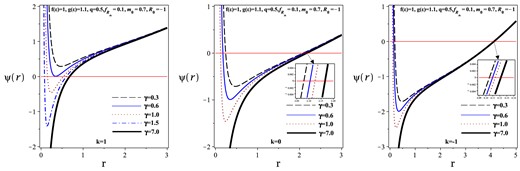
|$\psi (r)$| versus r for different values of k and |$\gamma$|.
For|$k=1$|: By considering constant values for the parameters of the studied system, there are two critical values for |$\gamma$|. Indeed, for |$\gamma \lt \gamma _{\rm{ critical}_{1}}$|, we find that the metric function has no roots. This implies that we have what is called a naked black hole. For |$\gamma =\gamma _{\rm{ critical} _{1}}$|, we observe the appearance of one root (in the extreme case). Considering |$\gamma _{\rm{ critical}_{1}}\lt \gamma \lt \gamma _{\rm{ critical}_{2}}$|, there are two roots for the metric function (as shown in the left panel of Fig. 1). It is important to note that the outer root corresponds to the event horizon, and its size increases with the ModMax parameter. In other words, as |$\gamma$| increases, the black hole becomes larger. Furthermore, the metric function has only one root when |$\gamma \gt \gamma _{\rm{ critical}_{2}}$| (as shown in the left panel of Fig. 1). It is worth mentioning that this root belongs to the event horizon. However, the black hole continues to grow in size as |$\gamma$| increases.
For|$k=0$|: Considering fixed values for the parameters of the studied system (as before), there exists a |$\gamma _{\rm{ critical}}$| such that the black hole has two horizons when |$\gamma \lt \gamma _{\rm{ critical}}$|. When |$\gamma$| is greater than |$\gamma _{\rm{ critical}}$|, the black hole has only one event horizon. It is worth noting that as |$\gamma$| increases, the event horizon also increases, resulting in the presence of larger black holes (see the middle panel in Fig. 1).
For|$k=-1$|: The behavior for |$k=-1$| is the same as for |$k=0$|. Specifically, when |$k=-1$|, there is a critical value for |$\gamma$| that determines whether black holes have one or two roots. If |$\gamma \lt \gamma _{\rm{ critical}}$|, there are two roots, but if |$\gamma \gt \gamma _{\rm{ critical}}$|, there is only one root. Additionally, as the value of |$\gamma$| increases, the event horizon expands, resulting in larger black holes (see the right panel in Fig. 1).
Our analysis of Fig. 1 indicates that large black holes belong to |$k=-1$|. Indeed, by considering the same values of parameters, for different values of k, the arrangement of the size of the radius of the black holes follows as |$r_{+}{}_{(k=-1)}\gt r_{+}{}_{(k=0)}\gt r_{+}{}_{(k=+1)}$|, where |$r_{+}$| is the radius of the event horizon.
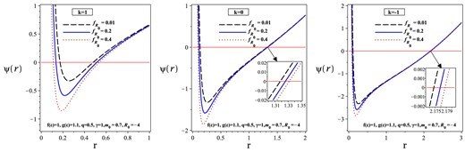
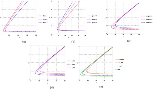
Here, we study the effects of the topological constant (k) and rainbow functions |$\mathrm{ f}\left(\varepsilon \right)$| and |$\mathrm{ g}\left(\varepsilon \right)$| on the obtained black holes. For this purpose, we plot Figs. 2 and 3. Our findings indicate that the large black holes belong to the case |$k=-1$|. Moreover, as |$\mathrm{ f}\left(\varepsilon \right)$| (|$\mathrm{ g}\left(\varepsilon \right)$| ) increases, the radius of the event horizon decreases (increases). In addition, by comparing the three panels in each of Figs. 2 and 3, we can see that the radius of the event horizon becomes more sensitive to an increase in |$\mathrm{ f}\left(\varepsilon \right)$| (|$g\left(\varepsilon \right)$|) when |$k=+1$| (|$k=-1$|).
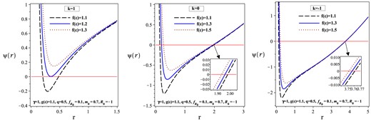
|$\psi (r)$| versus r for different values of k and |$\mathrm{ f}\left( \varepsilon \right)$|.

|$\psi (r)$| versus r for different values of k and |$\mathrm{ g}\left( \varepsilon \right)$|.
We study the effect of |$f_{R_{0}}$| (a parameter of |$\mathrm{ F}(R)$| gravity) by considering different topological constants in Fig. 4. As can be observed, the large black holes belong to the case |$k=-1$|, similar to the previous cases. However, increasing the value of |$f_{R_{0}}$| results in larger black holes. In fact, the radius of the event horizon of the black holes increases as the parameter of |$\mathrm{ F}(R)$| gravity is increased. Moreover, the radius of the black hole is more responsive in the case |$k=+1$|.
|$\psi (r)$| versus r for different values of k and |$f_{R_{0}}$|.
The effects of mass and electrical charge on the radius of the black hole are plotted in Fig. 5. Black holes with a large event horizon are associated with the topological constant |$k=-1$|. As the mass and electrical charge increase, the radius of the black hole’s event horizon also increases. In other words, larger black holes have greater masses and higher electrical charges.
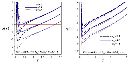
|$\psi (r)$| versus r for different values of k, q (left), and |$m_{0}$| (right). Three up diagrams are related to |$k=+1$|. Three middle diagrams belong to |$k=0$|. Also, three down diagrams for |$k=-1$|.
As a consequence of various parameters affecting the event horizon, larger black holes are classified as black holes with a negative topological constant (|$k=-1$|). These black holes possess greater mass, electric charge, |$\gamma$|, |$f_{R_{0}}$|, and |$\mathrm{ g}\left(\varepsilon \right)$| but lower |$\mathrm{ f}\left(\varepsilon \right)$|. On the other hand, our findings indicate that the radius of the event horizon is more sensitive for |$k=+1$| compared to other values of the topological constant (except when |$\mathrm{ g}\left(\varepsilon \right)$| increases, see Fig. 3).
3. Thermodynamics
Now, we are going to calculate the conserved and thermodynamic quantities of the topological black hole solutions in |$\mathrm{ F}(R)$| gravity’s rainbow to check the first law of thermodynamics.
For studying the thermodynamic properties of the obtained black hole solutions, it is necessary to express the mass (|$m_{0}$|) in terms of the radius of the event horizon |$r_{+}$| and the charge q as follows. Equating |$g_{tt}=\mathrm{ g}(r)$| to zero, we have
Here, we want to obtain the Hawking temperature for these black holes. The superficial gravity of a black hole is given by
where |$r_{+}$| is the radius of the event horizon. Considering the obtained metric function (28), and by substituting the mass (33) within Eq. (34), one can calculate the superficial gravity as
and by using the Hawking temperature as |$T=\frac{\kappa }{2\pi }$|, we can extract it in the following form:
Considering Eq. (36), we can study the behavior of the temperature in both the limit |$r_{+}\rightarrow 0$| (known as the high-energy limit) and the limit |$r_{+}\rightarrow \infty$| (known as the asymptotic behavior). The high-energy limit of the temperature is given by
which depends on the electrical charge, the parameter of the ModMax theory, the rainbow functions, and the parameter of |$\mathrm{ F}(R)$| gravity. Notably, the temperature is always negative in the high-energy limit. Therefore, the small black holes in this theory of gravity are not physical objects.
We expand our study to investigate the asymptotic behavior of the temperature, which leads to
As one can see, the temperature of large black holes depends on the rainbow functions (|$\mathrm{ g}\left(\varepsilon \right)$| and |$\mathrm{ f}\left(\varepsilon \right)$| ) and the constant scalar curvature (|$R_{0}$|). In order to have positive large black holes, we must consider |$R_{0}\lt 0$|.
When we consider |$T=0$| (Eq. (36)), we can find the temperature’s root (we show that by |$r_{_{T=0}}$|). Our analysis shows that there is only one real root, which can be expressed as follows:
According to the above equation, the root temperature of the black holes will become zero for a sufficiently large value of |$\gamma$| (or in the absence of an electrical charge).
As a result of our findings, in |$\mathrm{ F}(R)$|-ModMax gravity’s rainbow, the temperature of the large black holes can be positive and have only one root. It is notable that the temperature is negative before this root, and after it, the temperature becomes positive.
The electric charge of the black hole per unit volume, |$\mathcal {V}$|, can be obtained by using the Gauss law as
Considering |$F_{\mu \nu }=\partial _{\mu }A_{\nu }-\partial _{\nu }A_{\mu }$|, one can find the nonzero component of the gauge potential in which |$A_{t}=-\int F_{tr}dr$|, and therefore the electric potential at the event horizon (U) with respect to the reference (|$r\rightarrow \infty$|) is given by
In order to obtain the entropy of black holes in |$\mathrm{ F}(R)=R+\mathrm{ f}(R)$| theory, one can use a modification of the area law which means the Noether charge method [174],
where A is the horizon area and is defined as
So, the entropy of topological phantom AdS black holes per unit volume, |$\mathcal {V}$|, in |$\mathrm{ F}(R)$| gravity is given by replacing the horizon area (43) within Eq. (42) as
which indicates that the area law does not hold for the black hole solutions in |$R+\mathrm{ f}(R)$| gravity.
Using the Ashtekar–Magnon–Das (AMD) approach [175,176], we find the total mass of these black holes per unit volume, |$\mathcal {V}$|, in |$\mathrm{ F}(R)$| gravity as
where substituting the mass (33) within Eq. (45) yields
Here, we study the high-energy limit and asymptotic behavior of the mass. The high-energy limit of the mass is
which indicates that the high-energy limit depends on several factors, including the electrical charge (q), the ModMax theory (|$\gamma$|), the rainbow functions (|$\mathrm{ f}\left(\varepsilon \right)$| and |$\mathrm{ g}\left(\varepsilon \right)$|), and the parameter of |$\mathrm{ F}(R)$| gravity. Furthermore, it is important to note that the mass is always positive in this limit.
The asymptotic behavior is given by
where it is always positive because |$R_{0}\lt 0$|. As mentioned earlier in relation to temperature, in order to have a positive temperature, we need to consider |$R_{0}\lt 0$|. We now apply this condition to analyze the asymptotic behavior of mass. Consequently, the mass will always be positive as |$r_{+}\rightarrow \infty$|.
On the other hand, our analysis reveals an interesting behavior for middle black holes when |$k=-1$|. Specifically, the mass of middle black holes depends on the value of the topological constant. That is, |$M_{\rm{ middle}}\propto \frac{k\left(1+f_{R_{0}}\right) r_{+}}{8\pi \mathrm{ g}\left(\varepsilon \right) \mathrm{ f}\left(\varepsilon \right) }$|, and this relationship varies for different values of k, i.e.
which indicates that the total mass is always positive for |$k=+1$| and |$k=0$|. However, for |$k=-1$|, small and large black holes have positive mass, while the middle black holes encounter negative mass. This implies that there are two roots for |$k=-1$|, but no roots for |$k=+1$| or |$k=0$|. The roots of the mass (|$r_{1,2_{M=0}}$|) for |$k=-1$| are given by
where |$r_{1_{M=0}}$| and |$r_{2_{M=0}}$| refer to the smaller and larger roots of the mass, respectively. Our findings reveal that the mass of a black hole is positive in the ranges |$r_{+}\lt r_{1_{M=0}}$| and |$r_{+}\gt r_{2_{M=0}}$|. Additionally, it is negative between |$r_{1_{M=0}}$| and |$r_{2_{M=0}}$| (i.e. |$r_{1_{M=0}}\lt r_{+}\lt r_{2_{M=0}}$|).
It is straightforward to show that the conserved and thermodynamic quantities satisfy the first law of thermodynamics
where |$T=\left(\frac{\partial M}{\partial S}\right) _{Q}$| and |$U=\left(\frac{\partial M}{\partial Q}\right) _{S}$|, and they are in agreement with those calculated in Eqs. (36) and (41), respectively.
4. Thermodynamic topology and Duan’s |$\phi$| mapping theory
The main concept related to defects is the topological charge. In order to analyze the thermodynamic topology of a black hole, we compute the topological charge and use it to identify the topological classes. The specific method we employ to calculate the topological charge is known as Duan’s |$\phi$| mapping technique. The mathematical steps required for Duan’s |$\phi$| mapping technique are outlined in the following paragraph. From the expression for the off-shell free energy of a black hole, a vector field is constructed as follows [122]:
In the |$\phi ^{\Theta }$| component, the trigonometric function is chosen so that one zero point of the vector field can always be found at |$\theta = \frac{\pi }{2}$|. The other zero point can also be found by simply solving the equation, |$\phi ^{r}=0$|, which always results in |$\tau =\frac{1}{T}$|. The basic topological property associated with the zero point or topological defect of a field is its winding number or topological charge. In this work, we use Duan’s |$\phi$| mapping technique [177,178] to calculate the winding number. To find the topological charge we first determine the unit vectors n of the field in Eq. (52), which are
For the vector field, a topological current can be constructed in the coordinate space |$x^\nu =\lbrace t,r_+,\theta \rbrace$| as follows [177,178]:
where |$\partial _\nu =\frac{\partial }{\partial x^\nu }$| and |$\mu ,\nu ,\rho =0, 1, 2$|. The fundamental conditions that have to be fulfilled by the normalized vector |$n^a$| are [177,178]:
The current given in Eq. (54) is a conserved quantity, which can be verified by applying the current conservation law
It can be proved that the current |$j^{\mu }$| is only nonzero at the zero points of the vector field by using the following equation [122,177,178]:
where we use the following properties of the Jacobi tensor,
and the 2D Laplacian Green function,
Again, the topological charge W is related to the |$0^{\rm{ th}}$| component of the current density of the topological current through the following relation:
where |$w_{i}$| is the winding number around the zero point. Also, |$\beta {i}$| and |$\eta {i}$| are the Hopf index and the Brouwer degree, respectively. For the detailed derivation of the above formula the reader is referred to Refs. [177,178] or Ref. [122].
Hence, the topological charge is also nonzero only at the zero points of the vector field. To find the exact zero point where the topological charge is to be calculated, we plot the unit vector field n and find out the zero point at which it diverges. The zero point always turns out to be |$(\frac{1}{ T},\frac{\pi }{2}).$| Next, a contour is chosen around each zero point and is parameterized as
where |$\nu \in (0,2\pi )$|. In addition, |$r_{1}$| and |$r_{2}$| are the parameters that determine the size of the contour to be drawn, and |$r_{0}$| is the point around which the contour is drawn. |$r_{1}, r_{2}$|, and |$r_{0}$| are chosen in such a way that the contour C encloses the defect or zero point of the vector field n. After that, the deflection of the vector field n is found along the contour C as [121,122]:
This is followed by the calculation of the winding number |$w_{i}$| around the |$i^{\rm{ th}}$| zero point of the vector field, as follows:
Finally, the topological charge W can be determined by summing the winding numbers calculated along each contour around the zero points, i.e.
It is worth noting that when the parameter region does not have any zero points, the total topological charge is set to zero.
In the next two subsections, we will examine the thermodynamic topology of topological black holes in |$\mathrm{ F}(R)$|-ModMax gravity’s rainbow under two different ensembles: the fixed charge q ensemble and the fixed potential |$\phi$| ensemble. For each ensemble, we will determine the topological charge and analyze the impact of the ensemble choice and its corresponding thermodynamic parameter on the topological charge.
4.1. For elliptic (|$k=1$|) curvature hypersurface
4.1.1. Fixed charge (q) ensemble
For this ensemble, we calculate the off-shell free energy from Eqs. (44) and (46), which leads to
The components of the vector |$\phi$| are found to be
The unit vectors |$\left(n^{1},n^{2}\right)$| are computed using Eq. (53). Now we calculate the zero points of the |$\phi ^{r}$| component by solving |$\phi ^{r}=0$| and find an expression for |$\tau$| in the following form:
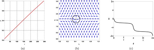
Next, we plot the horizon radius |$r_+$| against |$\tau$| in Fig. 6(a) for |$\mathrm{ f}(\varepsilon )=\mathrm{ g}(\varepsilon )=1.2$|, |$q=0.5$|, |$R_{0}=0.001$|, |$\gamma =0.5$|, and |$k=1$|. We observe two branches of black holes. In Fig. 6(b), a vector plot is shown for the components |$\phi ^{r}$| and |$\phi ^{\theta }$|, taking |$\tau =\tau {1}=60$|. The zero points of the vector field are observed at |$r_{+}=0.49089$| and |$r_{+}=4.70972$|. From Fig. 6(c), it can be seen that the winding number or topological charge corresponding to |$r_{+}=0.49089$| is |$+1$|, and the topological charge corresponding to |$r_{+}=4.70972$| is |$-1$|, represented by the solid lines in black and blue, respectively. Hence, the total topological charge is |$1-1=0$|. Additionally, an annihilation point is observed at |$(\tau {c} ,r_{+})=(15.1828, 0.8052)$|, represented by the black dot in Fig. 6(a).
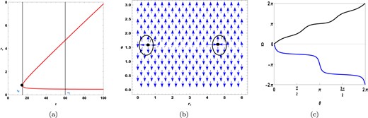
Topological charge of topological black holes |$(k=1)$| in fixed charge ensemble when positive values of |$R_{0}$| are considered.
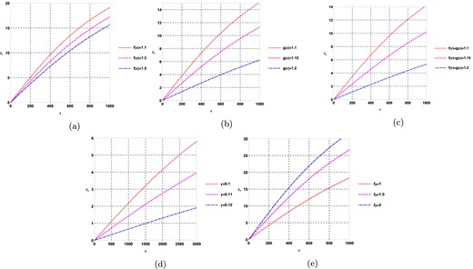
The topological charge remains invariant when varying the rainbow function, represented by |$\mathrm{ g}(\varepsilon )$|, |$\mathrm{ f}(\varepsilon )$|, |$\gamma$|, and |$f_{R_{0}}$|, while keeping |$q=0.5$|, |$R_{0}=0.001$|, and |$k=1$| fixed. In Fig. 7(a), the variation of |$\mathrm{ f}(\varepsilon )$| is shown with |$\mathrm{ g}(\varepsilon )=1$|, |$\gamma =0.5$|, and |$f_{R_{0}}=0.01$| fixed. In Fig. 7(b), the variation of |$\mathrm{ g}(\varepsilon )$| is shown with |$\mathrm{ f}(\varepsilon )=1$|, |$\gamma =0.5$|, and |$f_{R_{0}}=0.01$| fixed. Fig. 7(c) demonstrates the variation of both |$\mathrm{ f}(\varepsilon )$| and |$\mathrm{ g}(\varepsilon )$|, while keeping |$\gamma =0.5$| and |$f_{R_{0}}=0.01$| fixed. In Fig. 7(d), the variation of |$\gamma$| is shown with |$\mathrm{ f}(\varepsilon )=1.1,$||$\mathrm{ g}(\varepsilon )=1.1$|, and |$f_{R_{0}}=0.01$| fixed. Lastly, Fig. 7(e) illustrates the variation of |$f_{R_{0}}$| with |$\mathrm{ f}(\varepsilon )=1.5$|, |$\mathrm{ g}(\varepsilon )=1.5$|, and |$\gamma =0.5$| fixed. Based on Fig. 7, it is evident that the topological charge is consistently 0 across all cases.
|$\tau$| vs |$r_{+}$| plots for topological black holes |$(k=1)$| in fixed charge ensemble when positive values of |$R_{0}$| are considered.
If we consider the negative values of |$R_{0}$|, we observe a first-order phase transition, as shown in Fig. 8. Here, we plot |$\tau$| vs |$r_{+}$|, using the following values: |$f_{R_{0}}=0.001$|, |$\mathrm{ f}(\varepsilon )=1.2$|, |$\mathrm{ g}(\varepsilon )=1.2$|, |$q=1$|, |$R_{0}=-0.1$|, |$\gamma =0.5$|, and |$k=1$|. Figure 9 clearly displays three black hole branches. The small black hole branch is represented by the black solid LIne |$(0\le r_+ \le 1.6579)$|, the intermediate black hole branch is represented by the blue dashed line |$(1.6579 \lt r_+ \le 7.4061)$|, and the large black hole branch is represented by the red solid line |$(r_+ \gt 7.4061)$|. The winding numbers of these branches are shown in Fig. 9(d). The winding number for the large and small black hole branches is |$+1$|, whereas the intermediate black hole branch has a winding number of |$-1$|. A positive winding number indicates a stable branch, whereas a negative winding number indicates an unstable branch. The total topological charge is |$1-1+1=1$|.
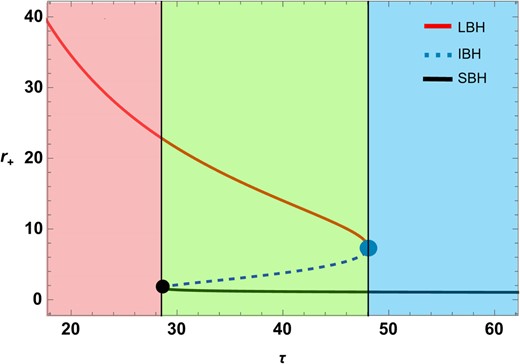
|$\tau$| vs |$r_{+}$| plots for topological black holes |$(k=1)$| in fixed charge ensemble for negative values of |$R_{0}$|.
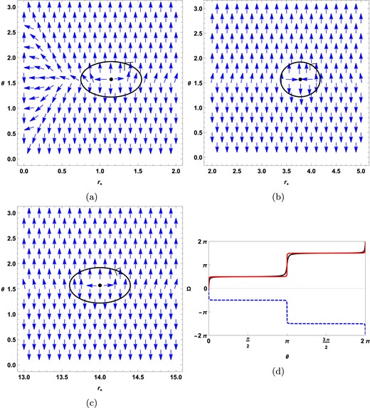
(a, b, c) Vector plots for zero points |$r_{+}=1.1478,r_{+}=3.7765,r_{+}=13.9994$|, respectively. (d) The winding number calculations for zero points |$r_{+}=1.1478,r_{+}=3.7765,r_{+}=13.9994$| are represented by a black solid line, a blue dashed line, and a red solid line, respectively.
It is observed that, apart from the sign of |$R_{0}$|, the topological charge is independent of other thermodynamic parameters. In conclusion, for topological black holes (|$k=1$|) in |$\mathrm{ F}(R)$|-ModMax gravity’s rainbow in the fixed charge ensemble, the topological charge is 0 for positive values of |$R_{0}$| and |$+1$| for negative values of |$R_{0}$|.
4.1.2. Fixed potential (|$\phi$|) ensemble
In this ensemble, the potential |$\phi$| is kept fixed, which is conjugate to charge q. The expression for |$\phi$| is obtained in the following form:
which is extracted from Eq. (46).
The new mass in this ensemble is given by
The free energy is obtained in the following form by using Eqs. (44) and (70):
By utilizing the equation |$\phi ^{r}=\frac{\partial \mathcal {F}}{\partial r_{+}}$| and the aforementioned relation, we can extract the component |$\phi ^{r}$| from the vector field in the following form:
By considering the above equation, the zero points of the |$\phi ^{r}$| component are obtained as
The plot in Fig. 10(a) shows the relationship between |$\tau$| and |$r_{+}$|. The parameter values used in this plot are as follows: |$f_{R_{0}}=0.01$|, |$\mathrm{ f}(\varepsilon )=1.1$|, |$\mathrm{ g}(\varepsilon )=1.1$|, |$\phi =0.05$|, |$R_{0}=0.001$|, |$\gamma =0.5$|, and |$k=1$|. Only one branch of the black hole is observed. In Fig. 10(b), a vector plot is displayed for the components |$\phi ^{r}$| and |$\phi ^{\theta }$| with |$\tau =150$|. The zero points of the vector field are located at |$r_{+}=0.41916$|. Fig. 10(c) shows that the topological charge corresponding to |$r_{+}=0.41916$| is |$-1$|, as indicated by the black line.
Topological charge of topological black holes |$(k=1)$| in the fixed potential ensemble when positive values of |$R_{0}$| are considered.
Similarly to the fixed q ensemble, the topological charge in this ensemble also remains unchanged when the rainbow function, represented by |$\mathrm{ g}(\varepsilon )$|, |$\mathrm{ f}(\varepsilon )$|, |$\gamma$|, and |$f_{R_{0}}$|, varies. However, the values of |$\phi$|, |$R_{0}$|, and k are fixed at 0.05, 0.001, and 1, respectively. Figure 11(a) illustrates the variation of |$\mathrm{ f}(\varepsilon )$| when |$\mathrm{ g}(\varepsilon )$| is held constant at 1, along with |$\gamma$| at 0.5 and |$f_{R_{0}}$| at 0.01. Similarly, in Fig. 11(b), the change in |$\tau$| versus |$r_{+}$| is shown when |$\mathrm{ g}(\varepsilon )$| is varied while keeping |$\mathrm{ f}(\varepsilon )$| at 1, |$\gamma$| at 0.5, and |$f_{R_{0}}$| at 0.01. Additionally, Fig. 11(c) demonstrates the impact of both |$\mathrm{ f}(\varepsilon )$| and |$\mathrm{ g}(\varepsilon )$| on the |$\tau$| versus |$r_{+}$| curve, while maintaining |$\gamma$| at 0.5 and |$f_{R_{0}}$| at 0.01. The variation of |$\gamma$| is depicted in Fig. 11(d), with fixed values of |$\mathrm{ f}(\varepsilon )$| at 1.5, |$\mathrm{ g}(\varepsilon )$| at 1.5, and |$f_{R_{0}}$| at |$0.01$|. Finally, Fig. 11(e) displays the variation of |$f_{R_{0}}$|, while holding constant values for |$\mathrm{ f}(\varepsilon )$|. Figure 11 indicates that due to the change in the ensemble, the topological charge shifts to |$-1$|, although it remains independent of thermodynamic quantities in this ensemble as well.
|$\tau$| vs |$r_+$| plots for topological black holes |$(k=1)$| in fixed potential ensemble when positive values of |$R_0$| are considered.
When negative values of |$R_{0}$| are considered, the topological charge changes to 0, as shown in Fig. 12. We have calculated the topological charge for the red-colored solid line in Fig. 12(a). The values used for calculations are: |$f_{R_{0}}=0.01$|, |$\mathrm{ f}(\varepsilon )=1.1$|, |$\mathrm{ g}(\varepsilon )=1.1$|, |$\phi =0.05$|, |$R_{0}=-0.01$|, |$\gamma =0.5$|, and |$k=1$|. A generation is observed at |$r_{+}=10.324$|, represented by the blue dot in Fig. 12(a). For |$\tau _{1}=200$|, the zero points are calculated at |$r_{+}=4.642$| and |$r_{+}=26.382$|, as shown in Fig. 12(b) and Fig. 12(c), respectively. In Fig. 12(d), the topological charge calculations for the zero points |$r_{+}=4.042$| and |$r_{+}=26.382$| are shown as black-colored and red-colored solid lines. It can be observed that the topological charge is 0.
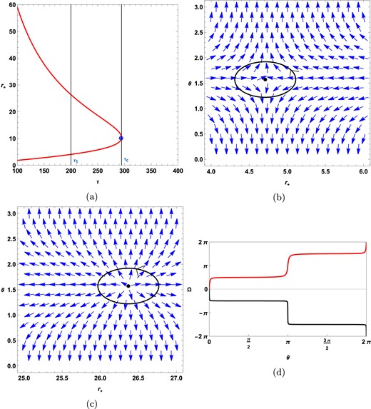
(a) represents the |$r_+$| vs |$\tau$| plot in which the |$\tau$| is the zero point of the vector field. Topological charge of topological black holes |$(k=1)$| in the fixed potential ensemble when negative values of |$R_0$| are considered. (b, c) Vector plots for the |$\mathrm{ f}( \varepsilon )=\mathrm{ g}( \varepsilon )=1.7$| case. (d) The red solid line and black solid line represent winding number calculations around the zero points |$r_+=4.042$| and |$r_+=26.382$|, respectively.
In Fig. 13, the graphs show the dependence of the nature of |$\tau$| vs |$r_{+}$| on thermodynamic parameters. Interestingly, in Fig. 13(b), a change in topological charge from 0 to 1 is observed when the parameter |$\mathrm{ g}(\varepsilon )$| is varied while keeping the other parameters fixed. For instance, in Fig. 13(b), the magenta dashed line represents the |$\tau$| vs |$r_{+}$| graph for |$f_{R}=0.01, \mathrm{ f}(\varepsilon )=1.6, \mathrm{ g}(\varepsilon )=141, \phi =0.05, R_{0}=-0.01$|, and |$\gamma =0.5$|. Here, a single black hole branch with a topological charge of |$+1$| is obtained. Therefore, when |$R_{0}$| is negative, the grand canonical ensemble yields two types of topological charge, namely 0 and |$+1$|, depending on the value of |$\mathrm{ g}(\varepsilon )$|.
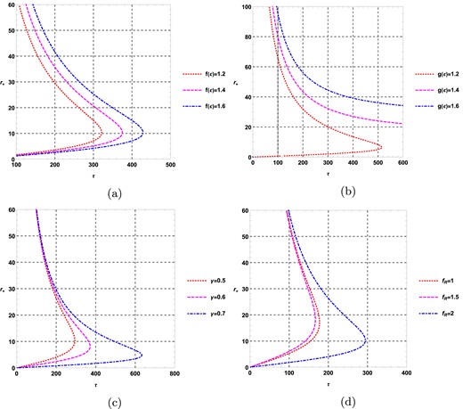
|$\tau$| vs |$r_+$| of topological black holes |$(k=1)$| in fixed potential ensemble when positive values of |$R_0$| are considered.
In conclusion, the topological charge for topological black holes with |$k=1$| in |$\mathrm{ F}(R)$|-ModMax gravity’s rainbow in the fixed potential ensemble is |$-1$| when a positive value of |$R_{0}$| is taken. Similarly, when negative values of |$R_{0}$| are considered, the topological charge is found to be 0 or |$+1$|. The results in both ensembles are summarized in Table 1.
Our results in two ensembles.
| Fixed charge |$(q)$| ensemble | Fixed potential |$(\phi )$| ensemble | |
|---|---|---|
| Topological charge | 0 or 1 | −1, 0, or +1 |
| Generation point | 0 or 1 | 1 or 0 |
| Annihilation point | 1 | 0 |
| Fixed charge |$(q)$| ensemble | Fixed potential |$(\phi )$| ensemble | |
|---|---|---|
| Topological charge | 0 or 1 | −1, 0, or +1 |
| Generation point | 0 or 1 | 1 or 0 |
| Annihilation point | 1 | 0 |
4.2. For flat (|$k=0$|) curvature hypersurface
For topological black holes with boundary of |$t=$| constant and |$r=$|constant having a flat curvature hypersurface, the equation for |$\tau$| becomes
It is clear from both the equations that |$\tau$| is always negative when |$R_{0}$| is positive. Therefore, to have a positive value of |$\tau$|, the scalar curvature |$R_{0}$| must be negative in both ensembles. Figures 14 and 15 show that the topological charge for the topological black hole with a flat curvature hypersurface in |$\mathrm{ F}(R)$|-ModMax gravity’s rainbow is 1 for both ensembles.
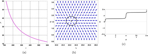
Plots for topological black holes |$(k=0)$| in the fixed charge ensemble at |$f_{R_{0}}=0.01, \mathrm{ f}( \varepsilon )=1.2, \mathrm{ g}( \varepsilon )=1.2, q=0.5, R_{0}=-0.01, \gamma =0.5$|, and |$k=0$|. (a) |$\tau$| vs |$r_{+}$| plot, (b) plot of vector field n on a portion of the |$r_{+}- \theta$| plane for |$\tau =300$|. The zero point is located at |$r_{+}=24.1362$|. (c) Computation of the contours around the zero point |$r_{+}=24.1362$| is shown in a black-colored solid line.

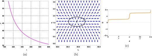
Plots for topological black holes |$(k=0)$| in the fixed potential ensemble at |$f_{R_{0}}=0.01, \mathrm{ f}( \varepsilon )=1.2, \mathrm{ g}( \varepsilon )=1.2, \phi =0.05, R_{0}=-0.01, \gamma =0.5$|, and |$k=0$|. (a) |$\tau$| vs |$r_{+}$| plot, (b) plot of vector field n on a portion of the |$r_{+}- \theta$| plane for |$\tau =300$|. The zero point is located at |$r_{+}=38.1417$|. (c) Computation of the contours around the zero point |$r_{+}=38.1417$| is shown in a blue-colored solid line.
4.3. For hyperbolic (|$k=-1$|) curvature hypersurface
For topological black holes with a boundary of constant t and constant r, characterized by a hypersurface with hyperbolic curvature, the equation for |$\tau$| can be expressed as
Due to the positive temperature condition, |$R_{0}$| must be negative. Figures 16 and 17 show the topological charge for the topological black hole with a hyperbolic curvature hypersurface in |$\mathrm{ F}(R)$| -ModMax gravity’s rainbow is 1 for both ensembles.
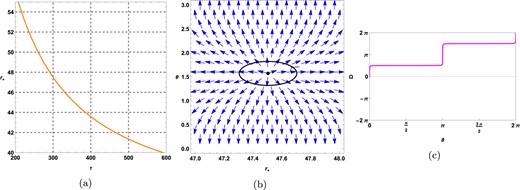
Plots for topological black holes |$(k=-1)$| in the fixed charge ensemble at |$f_{R_{0}}=0.01, \mathrm{ f}( \varepsilon )=1.2, \mathrm{ g}( \varepsilon )=1.2, q=0.5, R_{0}=-0.01, \gamma =0.5$|, and |$k=-1$|. (a) |$\tau$| vs |$r_{+}$| plot, (b) plot of vector field n on a portion of the |$r_{+}- \theta$| plane for |$\tau =300$|. The zero point is located at |$r_{+}=38.9266$|. (c) Computation of the contours around the zero point |$r_{+}=38.9266$| is shown in an orange-colored solid line.
Plots for topological black holes |$(k=-1)$| in the fixed potential ensemble at |$f_{R_{0}}=0.01, \mathrm{ f}( \varepsilon )=1.2, \mathrm{ g}( \varepsilon )=1.2, \phi =0.05, R_{0}=-0.01, \gamma =0.5$|, and |$k=-1$|. (a) |$\tau$| vs |$r_{+}$| plot, (b) plot of vector field n on a portion of the |$r_{+}- \theta$| plane for |$\tau =300$|. The zero point is located at |$r_{+}=47.5046$|. (c) Computation of the contours around the zero point |$r_{+}=47.5046$| is shown in a magenta-colored solid line.
5. Conclusion
In this paper, we investigated the effects of high energy and topological parameters on black holes in |$\mathrm{ F}(R)$| gravity, simultaneously. To achieve this objective, we took into account two corrections to |$\mathrm{ F}(R)$| gravity: (i) energy-dependent spacetime with different topological constants, and (ii) an NED field. In other words, we combined |$\mathrm{ F}(R)$| gravity’s rainbow with different topological constants and the ModMax NED theory to examine the impact of high energy and topological parameters on the physics of black holes. To begin with, we first extracted exact solutions in |$\mathrm{ F}(R)$|-ModMax gravity’s rainbow. To determine the singularities of the solutions obtained in the energy-dependent spacetime with different topological constants, we examined the Kretschmann scalar. Our calculations revealed the presence of an essential curvature singularity at the coordinate |$r=0$|. To analyze the asymptotic behavior of energy-dependent spacetime with different topological constants in the |$\mathrm{ F}(R)$|-ModMax theory of gravity, we examined the Kretschmann scalar and the metric function. Our findings indicated that the energy-dependent spacetime is asymptotically (A)dS when |$R_{0}=4\Lambda$|, and |$\Lambda \gt 0$| (|$\Lambda \lt 0$|). Moreover, this asymptotic behavior was independent of |$\gamma$| and k. In other words, the parameters of ModMax and the topological constant did not affect the asymptotic behavior of the energy-dependent spacetime, but it depended on the rainbow function |$\mathrm{ g}\left(\varepsilon \right)$|. The system we studied had various parameters that affected the event horizon. It has been observed that larger black holes are associated with a negative topological constant (|$k=-1$|). These black holes have high values for mass, electric charge, |$\gamma$|, |$f_{R_{0}}$|, and |$\mathrm{ g}(\varepsilon )$| but a lower |$\mathrm{ f}(\varepsilon )$|. Furthermore, our research has shown that changing specific parameter values makes the radius of the event horizon more sensitive to |$k=+1$| (except when |$\mathrm{ g}\left(\varepsilon \right)$| increases, see Fig. 3) when compared to other values of the topological constant.
In Sect. 3, we calculated the conserved and thermodynamic quantities of the topological black hole solutions in |$\mathrm{ F}(R)$| gravity’s rainbow to check the first law of thermodynamics. We determined the Hawking temperature, electrical charge, electrical potential, entropy, and total mass of these black holes. Subsequently, we confirmed that these thermodynamic quantities satisfy the first law of thermodynamics. By calculating the Hawking temperature, we discovered that only the larger black holes could have a positive temperature when |$R_{0}\lt 0$|. Furthermore, we found that the temperature had a single real root. The temperature was negative before this root but became positive afterwards. Additionally, our findings regarding the mass of these black holes revealed that for |$k=+1$| and |$k=0$|, this quantity was always positive. However, for |$k=-1$|, there were two roots at which the mass of large and small black holes was positive. Indeed, we encountered the positive mass of these black holes in the range |$r_{+}\lt r_{1_{M=0}}$| and |$r_{+}\gt r_{2_{M=0}}$| for |$k=-1$|. It was negative in the range |$r_{1_{M=0}}\lt r_{+}\lt r_{2_{M=0}}$|. This imposed the existence of two roots for the mass when |$k=-1$|.
In Sect. 4, thermodynamic topology was investigated in two ensembles. We used the off-shell free energy method, where black holes are assumed to be defects in their thermodynamic spaces. We studied the local and global topology of these black holes by computing the topological charges of the defects using Duan’s |$\phi$| mapping technique. It is observed that the topological charge for topological black holes with the boundary of |$t=$| constant and |$r=$| constant having an elliptic (|$k=1$|) curvature hypersurface in |$\mathrm{ F}(R)$|-ModMax gravity’s rainbow is 1 or 0 in the fixed charge ensemble and |$-1$| or 0 in the fixed potential ensemble depending upon the sign of |$R_0$|. On the other hand, black holes with the boundary of |$t=$| constant and |$r=$|constant having a flat (|$k=0$|) or hyperbolic (|$k=-1$|) curvature hypersurface have topological charge |$+1$| in both the ensembles. It is seen that, in a fixed charge ensemble, the topological charge is independent of variations in the respective thermodynamic parameters, except for the sign of |$R_0.$| Moreover, in a fixed |$\phi$| ensemble, the topological charge is found to be 0, |$-1$|, or |$+1$| for black holes with the boundary of |$t=$|constant and |$r=$|constant having an elliptic (|$k=1$|) curvature hypersurface. We observe that the topological classes of these black holes are dependent on the value of the rainbow function, the sign of the scalar curvature, and the choice of ensembles. On the other hand, in the fixed |$\phi$| ensemble, the topological charge is again found to be |$+1$| for black holes with the boundary of |$t=$| constant and |$r=$|constant having a flat (|$k=0$|) or hyperbolic (|$k=-1$|) curvature hypersurface. Hence, we can conclude that, based on the topological charge, topological black holes in |$\mathrm{ F}(R)$|-ModMax gravity’s rainbow can be classified into three topological classes: |$-1$|, 0, and |$+1$|. This classification depends on the choice of ensemble, the value of the topological parameter K, and the values of the thermodynamic parameters specific to the chosen ensemble.
Acknowledgement
B.E.P. would like to thank the University of Mazandaran. B.H. would like to thank DST-INSPIRE, Ministry of Science and Technology fellowship program, Govt. of India for awarding the DST/INSPIRE Fellowship [IF220255] for financial support.
Funding
Open Access funding: SCOAP3.
