Majorana-Free Bound State in the Continuum in the Double-Channel Fano–Anderson Structure

Abstract

1. Introduction

When confined quantum excitations are coupled to a band of continuous states, they generally undergo decay [1]. In view of this fact, researchers have always excepted the decay processes where a confined state lies in the continuum forever. Bound states in the continuum (BICs) were first predicted by von Neumann and Wigner in quantum mechanics [2]. They can be considered as a discrete solution of the single-particle Schrödinger equation in continuous states. Although BICs were originally proposed in quantum mechanics, they are predicted and observed in other wave systems such as optical waveguide [3–7], water wave [8–10], and acoustics [8], due to the fact that they are a universal wave phenomenon. Since BICs were observed, researchers have taken several experiments to explore them [11–13].

In addition to the importance of BICs in fundamental physics, they have also provided a wide range of applications, including lasing [14], sensing [15], and light trapping [16]. For example, Mao et al. obtained enantioselective resultant lateral forces and potential wells that can effectively separate enantiomers under the condition of linearly polarized light illumination [17]. One of the other technology applications is that researchers have implemented an effective laser with a finite-size cavity based on the idea of a supercavity mode generated by the combination of incidentally bound and symmetrically protected BICs in momentum space [18]. Also, there are projects to research BICs in high-coherence quantum optical devices. Two-level systems or quantum bits have been proposed to produce extremely long-lived and restricted single-photon excitations [19,20]. Besides, the emergence of BICs in mesoscopic strcture has also received extensive attention in the theoretical work [21–27], and researchers have discovered a bound state formed in a four-terminal junction [28]. Meanwhile, the appearance of BICs has been predicted in quantum waveguides with residue stubs [29–31].

Quantum dots (QDs), especially the mutually coupled multi-QD systems, exhibit more intricate electron transport behaviors, because they provide more Feynman paths for the electron transmission. When the size of a multi-QD system is shorter than or equal to the electron coherence length, quantum interference of electron waves through different Feynman paths leads to diverse transport properties. For example, in parallel-coupled QD systems, the coupling between the molecular states of QDs and the leads can be tuned by applying the appropriate magnetic flux or Rashba spin–orbit interactions, resulting in the Fano effect [32–35]. In some special cases, the phenomenon of so-called BICs occurs due to the complete decoupling of some molecular states from the leads. Based on the above, the incidence of BICs in a parallel-coupled QD system embedded in an Aharonov–Bohm (AB) interferometer is investigated, and the position of BICs is related to the adjustment of the threading magnetic flux [36,37]. In addition, the degeneracy of eigenlevels of the QDs in the QD ring also causes the BICs [38]. It is not difficult to find that the presence of BICs plays an important role in the quantum interference of QD structures. Therefore, we would like to look for BICs in some systems containing QDs.

In the present work, we would like to investigate the electron transport through a double-channel Fano–Anderson structure. It is found that the BIC phenomenon can be induced when interchannel QD–lead couplings are identical to the intrachannel dot–lead couplings, whose signature is manifested as a halved quantum transmission ability. If the balance between the dot–lead couplings is broken, the BIC result will also be destroyed, leading to the further suppression of the transmission ability. Moreover, motivated by the well-known transport properties of the Majorana bound state (MBS), we introduce it to this system in order to further observe the variation manner of the BIC phenomenon. Accordingly, it is found to cause the appearance of new dips in the transmission ability spectrum. The notable result is that the BIC is allowed to arise before the interchannel QD–lead couplings are tuned to equal the intrachannel couplings, when one MBS is coupled to the QD in this system. One can therefore understand the realization of BICs in coupled QDs and their variation due to the presence of side-coupled MBSs.

2. Theoretical model

Our considered system is shown in Fig. 1. The Hamiltonian that describes the electronic motion in the double-channel Fano–Anderson structure reads

The first term is the Hamiltonian for the noninteracting electrons in the two leads:

where |$c_{j\alpha k}^\dagger$|  |$( c_{j\alpha k})$| is an operator to create (annihilate) an electron of the continuous state |$k$| in lead-|$\alpha j$|⁠, and |$\varepsilon _{j\alpha k}$| is the corresponding single-particle energy. The second term describes the electron in the double QDs. It takes the form of

in which |$d^{\dagger }_{j}$|  |$(d_{j})$| is the creation (annihilation) operator of the electron in QD-|$j$|⁠, and |$\varepsilon _j$| denotes the electron level in the corresponding QD. |$U$| represents the interdot Coulomb interaction strength, |$n_{j}$| is the number of particles in the QD with |$n_{j}=d_{j}^\dagger d_{j}$|⁠, and |$t_c$| describes the interdot coupling. We assume that only one level is relevant in each QD with single-electron occupation, since we are only interested in the effects of interdot Coulomb interaction. The second part in Eq. (3) describes the coupling between QD-|$j$| and the corresponding MBS with |$\lambda _{j}$| being the coupling coefficient. Here, we take the low-energy effective Hamiltonian for the Majorana zero mode in the |$j$|th topological-superconducting nanowire, where |$\eta _{j}$| is the self-Hermitian operator for one MBS with |$\eta _{j}=\eta _{j}^\dagger$|⁠. |$\epsilon _{jm}$| represents the coupling between two MBSs at the end of the same topological superconductor. In our paper, we take |$\epsilon _{jm}=0$| to explore the properties of the zero mode.

The last term in the Hamiltonian denotes the electron tunneling between the leads and QDs. It is given by

where |$V_{j\alpha }$| and |$W_{j\alpha }$| denote the intrachannel and interchannel QD–lead coupling coefficients, respectively.

To study the electron-transport properties, we would like to adopt the nonequilibrium Green-function technique [39,40]. However, due to the presence of interdot Coulomb interaction, the Green function cannot be strictly solved. Thus, the approximation method should be introduced, whose feasibility is determined by the Coulomb strength.

For cases of weak or mediate Coulomb interaction, the Hartree–Fock or Hubbard-I approximations can be suitable to achieve a solution [41]. In such cases, the transmission ability is given as

with

which is identical to the noninteracting case. |$\mathrm{ T}^{ee}_{LR}$| describes the electron transmission between the two leads, whereas |$\mathrm{ T}^{eh}_{LL}$| corresponds to the local Andreev reflection in the left lead. |$\Gamma ^\alpha _{e(h)}$| is the matrix describing the coupling strength between the two QDs and the two leads. For instance, the elements of |$\Gamma ^\alpha _{e}$| are defined as follows: |$\Gamma ^{\alpha 1}_{11}=2\pi |V_{1\alpha }|^2\rho _{\scriptscriptstyle 0}(\omega )$|⁠, |$\Gamma ^{\alpha 1}_{12}=[\Gamma ^{\alpha 1}_{21}]^{*}=2\pi V_{1\alpha } W^{*}_{2\alpha }\rho _{\scriptscriptstyle 0}(\omega )$|⁠, and |$\Gamma ^{\alpha 1}_{22}=2\pi |W_{2\alpha }|^2\rho _{\scriptscriptstyle 0}(\omega )$|⁠; |$\Gamma ^{\alpha 2}_{11}=2\pi |W_{1\alpha }|^2\rho _{\scriptscriptstyle 0}(\omega )$|⁠, |$\Gamma ^{\alpha 2}_{12}=[\Gamma ^{\alpha 2}_{21}]^{*}=2\pi W_{1\alpha } V^{*}_{2\alpha }\rho _{\scriptscriptstyle 0}(\omega )$|⁠, and |$\Gamma ^{\alpha 2}_{22}=2\pi |V_{2\alpha }|^2\rho _{\scriptscriptstyle 0}(\omega )$|⁠. We can ignore the |$\omega$|-dependence of the element of |$\Gamma ^{\alpha }$| since the electron density of states |$\rho _{\scriptscriptstyle 0}(\omega )$| can be viewed as a constant in the wide-band limit. The retarded and advanced Green functions in Fourier space are involved in Eq. (6). Meanwhile, the Green functions are defined as follows: |$\mathrm{ G}_{jl}^r(t)=-i\theta (t)\langle \lbrace d_{j}(t),d_{l}^\dagger \rbrace \rangle$| and |$\mathrm{ G}_{jl}^a(t)=i\theta (-t)\langle \lbrace d_{j}(t),d_{l}^\dagger \rbrace \rangle$|⁠, where |$\theta (x)$| is the step function. The Fourier transforms of the Green functions can be performed via |${\mathrm{ G}_{jl}^{r(a)}(\omega )=\int ^{\infty }_{-\infty } \mathrm{ G}_{jl}^{r(a)}(t)e^{i\omega t}dt}$|⁠. These Green functions can be solved by the equation of motion method. We introduce an alternative notation |$\langle \!\langle A|B \rangle \!\rangle ^x$| with |$x=r$| or |$a$| to denote the Green functions in the Fourier space, e.g. |${\mathrm{ G}_{jl}^{r(a)}(\omega )}$| is identical to |$\langle \!\langle d_j|d^\dagger _l \rangle \!\rangle ^{r(a)}$|⁠, with |$\mathrm{ G}^r=[\mathrm{ G}^a]^\dagger$|⁠. The Green functions obey the following equation of motion:

Following this equation and by a straightforward derivation, we obtain the retarded Green functions, which are written in a matrix form as

Within the Hartree–Fock approximation, the Coulomb term only leads to the level shift of the QDs by causing |$\tilde{\varepsilon }_j=\varepsilon _j+U\langle n_{j^{\prime }}\rangle$|⁠, but does not induce any new change of the Green function matrix. When employing the Hubbard-I approximation to solve the Green functions, one can find that |$g_{je(h)}=[(\omega \mp \varepsilon _j)S^{}_{j e(h)}+i\Gamma _{jj,e(h)}]^{-1}$| with |$S_{je(h)}(\omega )=\frac{z\mp \varepsilon _{j}\mp U}{z\mp \varepsilon _{j}\mp U\pm U\langle n_{j^{\prime }}\rangle }$| [42,43]. The average electron occupation numbers in QDs are determined by the relations |${\langle n_{j}\rangle =\int d\omega [-{1\over \pi }\mathrm{Im} \mathrm{ G}^r_{jj}(\omega )]\mathrm{ f}(\omega )}$|⁠. |${\mathrm{ f}(\omega )=[\exp {\omega -\mu \over k_BT}+1]^{-1}}$| is the Fermi distribution with chemical potential |$\mu$|⁠, and it is simplified to be the step function (⁠|$\delta$|-function) at the zero-temperature case.

3. Numerical results and discussions

With the formulation developed in Sect. 2, we proceed to calculate the transmission ability spectra of our considered double-channel Fano–Anderson structure.

First of all, we concentrate on the transmission ability property by ignoring the MBS–QD couplings. Note that in such a case, |${\mathrm{ T}(\omega )=\mathrm{ T}^{ee}_{LR}(\omega )}$|⁠. Surely, with the help of the above derivation, one can write out the expression of the transmission ability. However, due to its complicatedness, we would like to present the transmission coefficients in the respective channels, i.e. |${\mathrm{ T}(\omega )=\sum _{jl}|{\bf t}_{jl}|^2}$| with

In our system, we would like to differentiate the intrachannel couplings from the interchannel couplings by supposing |$\Gamma ^{\alpha 1}_{11}=\Gamma ^{\alpha 2}_{22}=\Gamma _{{\scriptscriptstyle V}}$| and |$\Gamma ^{\alpha 1}_{22}=\Gamma ^{\alpha 2}_{11}=\Gamma _{{\scriptscriptstyle W}}$|⁠. Accordingly,

under the condition of real |$t_c$|⁠. It is not difficult to find that |$S_j$| originates from the contribution of the Coulomb term within the Hubbard-I approximation. For the case of weak Coulomb interaction, we can handle the many-body term within the Hartree–Fock approximation. In such a case, |$g_{j}$| has the same form as the zero-Coulomb result, except that |$\varepsilon _j$| should be changed to be |$\tilde{\varepsilon }_j=\varepsilon _j+U\langle n_{j^{\prime }}\rangle$|⁠.

Prior to calculation, we would like to state the parameter unit by taking |$\Gamma _{{\scriptscriptstyle V}}=1.0$|⁠. Also, to facilitate the calculation, we introduce |$\delta$| to fix the magnitude of the QD levels, i.e. |$\varepsilon _{1}=\varepsilon -\delta$| and |$\varepsilon _{2}=\varepsilon +\delta$|⁠. Figure 2 shows the transmission ability spectra of |$U=0$| and |$\varepsilon =\delta =0$| in the absence of local magnetic flux. In such a case, we have

In Fig. 2(a) one can find that under the condition of |$\Gamma _{{\scriptscriptstyle W}}=0$|⁠, the effect of increasing |$t_c$| is to suppress the magnitude of the transmission ability and induce a symmetric double-peak profile in its spectrum. When |$\Gamma _{{\scriptscriptstyle W}}=0.5$|⁠, the transmission ability spectrum displays one peak at |$\omega =0$|⁠. With the increase of |$t_c$|⁠, this peak shifts gradually to the negative-energy direction. And also, the peak magnitude suffers from a corresponding decrease. Next, as |$\Gamma _{{\scriptscriptstyle W}}$| gets close to |$\Gamma _{{\scriptscriptstyle V}}$|⁠, the transmission ability peak is narrowed very much. This should certainly be attributed to the further localization of the eigenstate of the double QDs. Accordingly, if we take |$\Gamma _{{\scriptscriptstyle W}}=\Gamma _{{\scriptscriptstyle V}}$|⁠, the resonant peak is eliminated and the whole transmission ability spectra exhibit the Breit–Wigner lineshape with the maximum being 1.0. This exactly means that with the increase of interchannel QD–lead coupling, the BIC phenomenon comes into being, which is independent of the change of interdot coupling. This result can be analytically expressed, since |${\bf t}_{11}={\bf t}_{12}={2\Gamma _{{\scriptscriptstyle V}}\over (\omega -\varepsilon -t_c)+4i\Gamma _{{\scriptscriptstyle V}}}$|⁠.

Fig. 1.

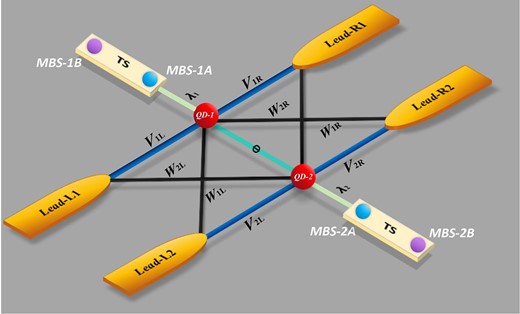
Schematic of the double-QD Fano–Anderson structure. In this system, only one level is considered in each QD with its single-electron occupation. The QD–lead coupling coefficients are defined by |$V_{j\alpha }$|⁠, and the interdot coupling is denoted as |$t_c$|⁠. Two MBSs contributed by two topological-superconducting nanowires are introduced, side-coupled to the QDs, respectively. Since the Majorana zero mode is considered, the other MBS in each nanowire is decoupled from this system.

Open in new tabDownload slide

Fig. 2.

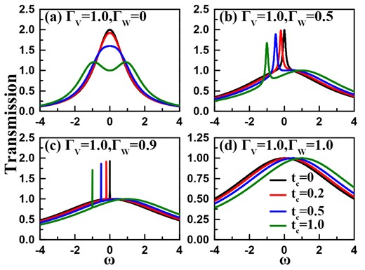
Spectra of the transmission ability in the coupled Fano–Anderson system. The structure parameters are taken to be |$\varepsilon =\delta =0$| and |$\phi =0$|⁠. (a)–(d) Results of |$\Gamma _{{\scriptscriptstyle W}}=0$|⁠, 0.5, 0.9, and 1.0, respectively.

Open in new tabDownload slide

In Fig. 3, we consider the influence of QD-level detuning on the transmission ability spectra. Without loss of generality, the interdot coupling is taken to be 0.5. Firstly, the results in Fig. 3(a) show that in the case of |$\Gamma _{{\scriptscriptstyle W}}=0$|⁠, the QD-level detuning plays the same role as the interdot coupling in modifying the transmission ability spectra. Namely, the peak around the point of |$\omega =0$| is suppressed gradually, accompanied by the splitting of it. However, in the cases of |$\Gamma _{{\scriptscriptstyle W}}\ne 0$|⁠, the level detuning modifies the transmission ability spectra in a clearer way, as shown in Fig. 3(b)–(c). The nonzero |$\delta$| causes the peak to transit into the dip in the transmission ability spectra; such a phenomenon is more apparent with the increase of |$\Gamma _{{\scriptscriptstyle W}}$|⁠. At the critical case where |$\Gamma _{{\scriptscriptstyle W}}=1.0$|⁠, the BIC result is transformed into the Fano antiresonance, and the antiresonance valley is widened following the increase of |$\delta$|⁠. Despite the destruction of the BIC, the magnitude of the transmission ability remains equal to 1.0. We then get a basic understanding about the QD-level detuning in this system.

Fig. 3.

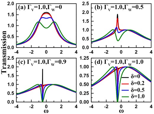
Transmission function spectra of the coupled Fano–Anderson system. The structure parameters are taken to be |$\varepsilon =0$|⁠, |$t_c=0.5$|⁠, and |$\phi =0$|⁠. (a)–(d) Results of |$\Gamma _{{\scriptscriptstyle W}}=0$|⁠, 0.5, 0.9, and 1.0, respectively.

Open in new tabDownload slide

On the other hand, we present the effect of local magnetic flux on the quantum ability in our structure. Note that in the case of |$\Gamma _{{\scriptscriptstyle W}}=0$|⁠, the quantum ring of this system is broken, so the magnetic flux makes zero contribution to the change of the transmission ability curve [see Fig. 4(a)]. In the case of nonzero |$\Gamma _{{\scriptscriptstyle W}}$|⁠, finite magnetic flux leads to the apparent suppression of the transmission ability magnitude. Such a result is similar to the effect of QD-level detuning, as shown in Fig. 4(b)–(c). However, note that magnetic flux also takes an effect different from QD-level detuning. On the one hand, when the magnetic flux phase factor increases, the suppression of transmission ability is relatively apparent, especially on the negative-energy side of the transmission dip. It shows that the quantum transmission can almost not display any peak in such case. On the other hand, the dip valley is widened seriously. For instance, in the case of |$\phi ={2\pi /3}$|⁠, the transmission ability shows up as the asymmetric lineshape. All these phenomena are visible in Fig. 4(d). One can find that local magnetic flux can also destroy the BIC phenomenon, and induce the Fano antiresonance.

Fig. 4.

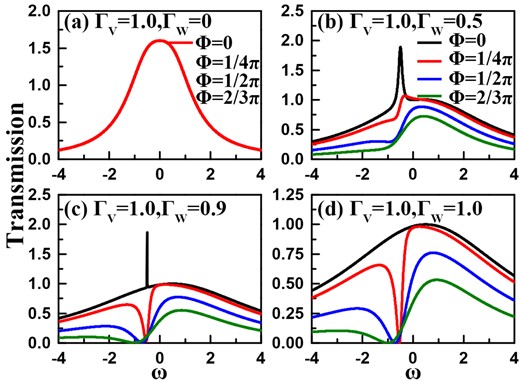
Transmission ability spectra of the coupled Fano–Anderson system. The structure parameters are taken to be |$\varepsilon =\delta =0$| and |$t_c=0.5$|⁠. (a)–(d) Results of |$\Gamma _{{\scriptscriptstyle W}}=0$|⁠, 0.5, 0.9, and 1.0, respectively. In each figure, the magnetic flux phase factor is taken to be |$\phi =0$|⁠, |${\pi \over 4}$|⁠, |${\pi \over 2}$|⁠, and |${2\pi \over 3}$|⁠.

Open in new tabDownload slide

To understand the properties of the transmission ability and the appearance of the BIC results, we would like to investigate the density of states (DOS) in this system. In Fig. 5(a)–(b), we take |$\varepsilon =0$| and |$t_c=0.5$| to present the DOS spectra in the cases of |$\Gamma _{{\scriptscriptstyle W}}=0.5$| and 1.0, respectively. It can be found that when |$\Gamma _{{\scriptscriptstyle W}}=0.5$|⁠, the DOS peak is located around the position of |$\omega =-0.5$|⁠. With the increase of |$\delta$|⁠, the DOS peak is suppressed accordingly, accompanied by the widening of it. We thus understand that the QD-level detuning changes the properties of the quantum states in this system, leading to the modification of the quantum transmission results. A similar phenomenon can also be observed in Fig. 5(b). In the case of |$\delta =0$|⁠, the DOS spectrum almost displays a |$\delta$|-function lineshape, which means the complete localization of the quantum state at |$\omega =-0.5$|⁠. In fact, for the coupled double-QDs, we can obtain the eigenlevels as |$E_{\pm }=\varepsilon \pm \sqrt{\delta ^2+t_c^2}$|⁠. This suggests that the bonding state contributes to the DOS peak, and its complete localization gives rise to the appearance of the BIC phenomenon. The increase of |$\delta$| causes the bonding state to shift in the low-energy direction, thus the position of the DOS peak is dependent on the value of |$\delta$|⁠, as shown in Fig. 5(a). On the other hand, regarding the role of magnetic flux, one can see in Fig. 5(c)–(d) that it only leads to the widening and suppression of the DOS peak, but cannot change the position of the DOS peak. Surely, as shown in Fig. 5(c), the DOS peak is destroyed seriously with the increase of magnetic flux. This helps us to understand the modification of the transmission ability spectra in Fig. 4.

Fig. 5.

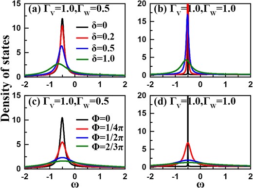
DOS spectra of the two-channel Fano–Anderson structure. The parameters are taken to be |$\varepsilon =0$| and |$t_c=0.5$|⁠. (a)–(b) Results of |$\Gamma _{{\scriptscriptstyle W}}=0.5$| and 1.0, following the change of the QD-level detuning. (c)–(d) DOS results of |$\delta =0$| with the change of the magnetic flux.

Open in new tabDownload slide

It is well known that the peaks in the transmission spectra are determined by the molecular states of the “coupled atoms” (i.e. the QDs) in the scattering region. Therefore, it is necessary for us to solve the molecular states and rewrite the Hamiltonian in the molecular orbital representation, to clarify the occurrence of the BIC phenomenon. For our system, if |$\delta = 0$|⁠, the unitary matrix relating the molecular states and the “coupled atoms” can be expressed directly, i.e. |$[{\boldsymbol \eta }]={1\over \sqrt{2}}\left [ {_{\ 1}^{-1}}\quad {_{1}^{1}} \right ]$|⁠. And then, the new expression of |$H$| is given as |$H=H_C+H_{D^{\prime }}+H_{T^{\prime }}$|⁠, where

with |$\tilde{\tau }^{L}_{11(2)}=[\boldsymbol \eta ]^\dagger _{21}V_{1(2)L}+[\boldsymbol \eta ]^\dagger _{11}W_{1(2)L}$|⁠, |$\tilde{\tau }^{R}_{11(2)}=[\boldsymbol \eta ]^\dagger _{21}V_{1(2)L}+[\boldsymbol \eta ]^\dagger _{11}W_{1(2)L}$|⁠, |$\tilde{\tau }^{L}_{21(2)}=[\boldsymbol \eta ]^\dagger _{22}V_{1(2)L}+[\boldsymbol \eta ]^\dagger _{12}W_{1(2)L}$|⁠, and |$\tilde{\tau }^{R}_{21(2)}=[\boldsymbol \eta ]^\dagger _{22}V_{1(2)L}+[\boldsymbol \eta ]^\dagger _{1 2}W_{1(2)L}$|⁠. With the help of these results, one can understand that the weak coupling between the bonding state (i.e. |$f^\dagger _1|0\rangle$|⁠) and the leads provides the resonant channels for the intrawaveguide transmission and the Fano interference in the interwaveguide transmission. Instead, the antibonding state |$f^\dagger _2|0\rangle$| offers the reference channels. In the critical case where |$V_{j\alpha }=W_{j\alpha }$|⁠, the bonding state will be decoupled from the leads, leading to the occurrence of the BIC. Up to now, the leading transmission results in this structure have been clarified. To be concrete, the decoupling effect induces the occurrence of the BIC phenomenon.

Following the noninteracting results, we take the interdot Coulomb interaction into account, to investigate its impact on the transmission ability property in the two-channel Fano–Anderson structure. In the case of weak Coulomb interaction, the Coulomb term can be managed within the Hartree–Fock approximation. The results are shown in Fig. 6(a)–(d), where the Coulomb strength is taken to be |$U=0.2$|⁠. In these figures, it can be found that the transmission ability spectra are basically similar to those in the noninteracting case, regardless of the settings of the structural parameters. As for the Coulomb-induced changes in the transmission ability spectra, they are mainly manifested as follows. On the one hand, the Coulomb interaction causes the transmission ability spectra to shift in the high-energy direction. Such a result should be attributed to the addition of the QD levels within the Hartree–Fock approximation, i.e. |$\varepsilon _j\rightarrow \varepsilon _j+U\langle n_{j^{\prime }}\rangle$|⁠. Note that since the average electron number in the QD is determined by the structural parameter of the whole system, the transmission dip experiences a weak right shift in such a case. On the other hand, the transmission peak in the case of |$\Gamma _{{\scriptscriptstyle W}}=0.9$| becomes weaker than the noninteracting case. In view of this fact, we take |$U=0.5$| to present the change of the transmission function spectra, as shown in Fig. 6(e)–(f). It can be readily found that in such a case, the transmission peak contributed by the bonding state becomes more ambiguous even in the case of |$\Gamma _{{\scriptscriptstyle W}}=0.9$|⁠.

Fig. 6.

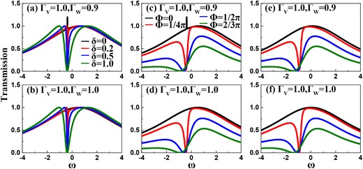
Transmission ability spectra of our structure, in the presence of weak interdot Coulomb interaction. The parameters are |$\varepsilon =0$| and |$t_c=0.5$|⁠. (a)–(b) Results of |$U=0.2$| with |$\Gamma _{{\scriptscriptstyle W}}=0.9$| and 1.0, following the change of the QD-level detuning. (c)–(d) Transmission ability curves of |$\delta =0$|⁠, in the case of |$U=0.2$|⁠. (e)–(f) Results of |$\delta =0$| with |$U=0.5$|⁠.

Open in new tabDownload slide

To further verify the effect of the interdot Coulomb interaction, we would like to increase the interdot Coulomb strength to present the BIC signature in the transmission ability spectra. The results are exhibited in Fig. 7, where the Coulomb strength is |$U=2.0$|⁠. Due to the increased Coulomb strength, we handle the interdot electron interaction within the Hubbard-I approximation in these cases. Note that within such an approximation, the effect of Coulomb interaction is to cause the splitting of the QD levels. Accordingly, more channels can be built to assist the quantum transmission in this structure, compared with the noninteracting and weak-Coulomb cases. Therefore, we see the severe oscillation of the transmission ability spectra, as shown in Fig. 7(a)–(c). It should be noticed that regardless of adjustment of the structural parameters and the presence of local magnetic flux, the transmission maximum is only equal to 1.0 under the condition of |$\Gamma _{{\scriptscriptstyle W}}=0.9$|⁠. This precisely means that in the case of |$\delta =\phi =0$|⁠, the BIC phenomenon is allowed to take place, even in the case of |$\Gamma _{{\scriptscriptstyle W}}=0.9$|⁠. Regarding the transmission dip in such a case, it should be attributed to the Coulomb-induced QD level splitting. On the other hand, in the presence of nonzero |$\delta$| or |$\phi$|⁠, the BIC phenomenon can be destroyed directly. As shown in Fig. 7(b)–(c), the apparent transmission dips come into being. Instead, in such cases, the magnetic flux modifies the transmission ability spectra in a substantial way. The Coulomb-induced spectral division is erased, and one clear peak near |$\omega =1.0$| arises, which tends to be more resonant with the increase of magnetic flux. Up to now, we can understand that in the case of stronger interdot Coulomb interaction, the BIC result is allowed to occur earlier, before the interchannel QD–lead coupling equals the intrachannel coupling completely. In addition, the role of magnetic flux tends to be more complicated in modulating the transmission ability spectra.

Fig. 7.

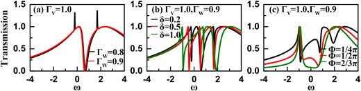
Transmission function spectra with stronger interdot Coulomb interaction |$U=2.0$|⁠. (a) Results of |$U=2.0$| with |$\Gamma _{{\scriptscriptstyle W}}=0.8$| and 0.9, respectively, without QD-level detuning or magnetic flux. (b)–(c) Transmission function curves of nonzero QD-level detuning and magnetic flux, respectively.

Open in new tabDownload slide

In the following, we would like to introduce MBSs to couple laterally to the QDs, to observe the variation of the transmission ability spectra. The reason is that the Majorana fermion is half a Dirac fermion, thus when MBSs are coupled to the QD circuit, lots of interesting transport results have been reported. Our expectation is to manipulate the BIC by considering the coexistence of electron tunneling and local Andreev reflection. To get a clear description, we would like to perform our discussion by considering it from two aspects. Firstly, we consider two MBSs to be coupled to the QDs, respectively, with |$\lambda _j=\lambda$|⁠. On the other hand, only one MBS is introduced to be connected to one QD.

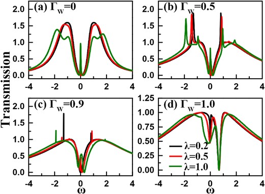
In Fig. 8(a), we present the transmission ability spectra in the former case. Accordingly, it shows that in the case of |$\Gamma _W=0$|⁠, the coupling of MBSs causes the decrease of the transmission function magnitude from 2.0 to 1.0 at the zero-energy limit. Such a result should be attributed to the occurrence of equivalent electron tunneling and local Andreev reflection in the presence of MBSs. With the increase of MBS–QD coupling, the zero-energy transmission ability is always fixed, although its spectrum changes obviously. When |$\lambda =1.0$|⁠, the widening of the transmission ability spectrum leads to the formation of a halved transmission ability peak. As |$\Gamma _{{\scriptscriptstyle W}}$| changes to be 0.5, in Fig. 8(b) we find the transmission ability spectrum generates one notable peak in the negative-energy region, with the halving of the transmission ability in the other region. The other phenomenon is that as the MBS–QD coupling strength increases, the peak value turns to be smaller. In the vicinity of |$\omega =0$|⁠, additional oscillation is formed in the transmission ability spectra, due to the side-coupling of MBSs. When continuing to increase |$\Gamma _{{\scriptscriptstyle W}}$|⁠, we see that the width of the peak is almost vanished and the transmission valley becomes clearer around the position of |$\omega =0$|⁠. Compared with the previous cases in Figs. 3 and 4, the appearance of MBSs tends to be helpful for the formation of the BIC. Next, in the critical case where |$\Gamma _{{\scriptscriptstyle W}}=\Gamma _{{\scriptscriptstyle V}}$|⁠, the results in Fig. 8(d) show the perfect BIC phenomenon, with transmission equal to 0.5 at the zero-energy limit.

Fig. 8.

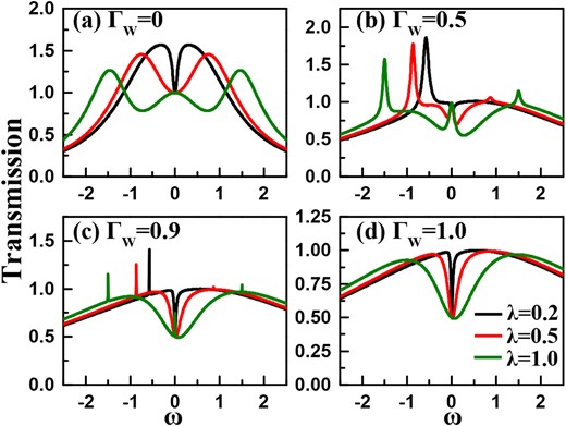
Transmission ability spectra of the coupled Fano–Anderson system in the presence of side-coupled MBSs. The parameters are taken to be |$\varepsilon =0$|⁠, |$\delta =0$|⁠, and |$t_c=0.5$|⁠. (a)–(d) Results of |$\Gamma _{{\scriptscriptstyle W}}=0$|⁠, 0.5, 0.9, and 1.0, respectively.

Open in new tabDownload slide

In Fig. 9, we consider the latter case where only one MBS is coupled to the Fano–Anderson structure. The corresponding parameters are taken to be |$\lambda _{1}=0$| with |$\lambda _{2}=0.2$|⁠, 0.5, and 1.0, respectively. Firstly, Fig. 9(a) shows the result of |$\Gamma _{{\scriptscriptstyle W}}=0$|⁠. It can be found that when only one MBS is present, the transmission ability spectra experience a similar change, compared with the case of two MBSs. The main difference is that the zero-energy transmission value remains equal to 1.29, independent of the increase of the MBS–QD coupling strength. The reason is due to the fact that in the case of only one MBS, the Green’s functions in the zero-bias limit are expressed as

The changes in the forms of the Green’s functions lead to a nonquantized transmission ability value at the zero-energy limit. Also, we know that the zero-energy transmission ability is independent of the coupling strength between the QD and MBS. Next, when |$\Gamma _W=0.5$|⁠, in Fig. 9(b) it shows that the transmission ability spectra display one peak in the negative-energy region. Different from the results in Fig. 8(b), the peak width is relatively apparent. With the increase of |$\lambda _2$|⁠, this transmission peak is suppressed and widened seriously. In the case of |$\lambda _2=1.0$|⁠, the magnitude of transmission ability is decreased below 1.0. As |$\Gamma _{{\scriptscriptstyle W}}$| changes to 0.9, the spectrum exhibits one narrow peak when the coupling strength is taken to be |$\lambda _{2}=0.2$|⁠. Once the MBS–QD coupling increases to 0.5, the transmission peak disappears and the transmission magnitude keeps below 1.0. This also suggests a nontrivial modification effect of the MBS on the transmission in this case. At the same time, three dips can be observed in the transmission ability spectra, and their widths are also proportional to the MBS–QD coupling. Such a result becomes more notable in the case of |$\Gamma _W=1.0$|⁠, as shown in Fig. 9(d). It can also be found that at the position of transmission dips, the transmission values are 0.5 approximately. In comparison with the results in Fig. 8, one can know that introducing one MBS to couple to the Fano–Anderson system plays a different role in modulating the transmission ability spectra. Even in the case of weak asymmetry of the QD–lead couplings, the transmission ability magnitude can be efficiently suppressed.

Fig. 9.

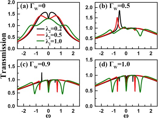
Transmission ability spectra of the coupled Fano–Anderson system with one side-coupling MBS. The parameters are taken to be |$\varepsilon =0$|⁠, |$\delta =0$|⁠, and |$t_c=0.5$|⁠. (a)–(d) Results of |$\Gamma _{{\scriptscriptstyle W}}=0$|⁠, 0.5, 0.9, and 1.0, respectively. The coupling strengths between the two QDs are |$\lambda _{1}=0$| and |$\lambda _{2}=0.2$|⁠, 0.5, and 1.0.

Open in new tabDownload slide

Similar to the MBS-absent case, in Fig. 10 we would like to present the DOS results of the QDs in the cases of QD–MBS couplings, for further understanding how the BIC results are modified by the MBSs. In Fig. 10(a)–(b), it shows the DOS results when two MBSs are side-coupled to the QDs in a symmetric way, in the cases of strong and weak QD–lead couplings. The QD–MBS coupling parameters are the same as those in Fig. 8(d). One can find that in the case of strong QD–lead coupling, three peaks always exist in the DOS spectra, and their distances are increased following the enhancement of the QD–MBS coupling strength. To explain this phenomenon, we would like to solve the system eigenlevels, which are expressed as |$E_{1(2)}=-\sqrt{2\lambda ^2+t_c^2}$|⁠, |$E_{3(4)}=0$|⁠, and |$E_{5(6)}=\sqrt{2\lambda ^2+t_c^2}$|⁠. It can be readily found that the eigenstates are twofold degenerate. According to previous works [44], the twofold degeneracy certainly causes one eigenstate to decouple from the QD system. We then understand that the sharp peaks originate from the decoupled eigenstates. Therefore, when two MBSs are coupled to the QDs, respectively, a new BIC mechanism is induced. However, such a type of BIC is determined by the QD–MBS coupling manner but not the QD–lead coupling symmetry. Since three eigenstates are coupled to the leads, in Fig. 8(a) we see three peaks in the transmission ability spectra. Regarding the effect of the increase of |$\Gamma _W$|⁠, it is similar to the MBS-absent case. To be concrete, the transmission peak in the negative-energy region is enhanced then narrowed, until its disappearance at the case of |$\Gamma _W=\Gamma _V=1.0$|⁠. Surely this BIC result, governed by the QD–lead coupling manner, can be understood with the help of the theory in the above paragraphs. To further present the decoupling eigenstates, we plot the DOS spectra in the case of weak QD–lead coupling in Fig. 10(b). It shows that the decoupling eigenstates correspond to the additional sharp peaks without any widening. Meanwhile, we know in Fig. 10(a) that due to the strong coupling between three eigenstates and the leads, the DOS minimum remains greater than zero in a large energy region. As a comparison, Fig. 10(c)–(d) show the DOS results of a MBS side-coupled to one QD, e.g. QD-2. To begin with, we would like to present the eigenlevels in such a case, i.e. |$E_{1}=-\sqrt{2\lambda ^2_2+t_c^2}$|⁠, |$E_{2}=-t_c$|⁠, |$E_{3}=0$|⁠, |$E_{4}=t_c$|⁠, and |$E_{5}=\sqrt{2\lambda ^2_2+t_c^2}$|⁠, respectively. In Fig. 10(c)–(d), it is clearly observed that in the case of strong QD–lead coupling, only the four-peak structure is formed following the increase of QD–MBS coupling to be |$\lambda _1=1.0$|⁠. Besides, the DOS peak for |$E_1$| is seriously suppressed and widened by the enhancement of the QD–lead coupling symmetry. With the help of the results in Fig. 10(d), one can see that the DOS peak for |$E_2$| is covered for the small |$\lambda _1$|⁠. In the case of |$\lambda _1=1.0$|⁠, the five-peak DOS spectrum comes into being. Thus, we know that in the case of one MBS, no eigenstate contributes to the BIC result. By further observing the results in Fig. 9, we know that the transmission peak corresponding to |$E_1$| is widened and suppressed as |$\Gamma _W$| increases, until its value is smaller than 1.0. As for the DOS peak of |$E_2$|⁠, it is exactly covered by the DOS peak of |$E_1$| completely due to the strong QD–lead coupling, so it has no correspondence in the transmission ability spectra in Fig. 9.

Fig. 10.

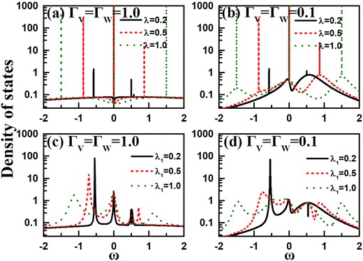
DOS spectra in the presence of side-coupled MBSs. (a)–(b) Results of two MBSs in the cases of |$\Gamma _W=\Gamma _V=1.0$| and |$\Gamma _W=\Gamma _V=0.1$|⁠, respectively. (c)–(d) The corresponding results in the presence of one MBS. The parameters are taken to be |$\varepsilon =0$|⁠, |$\delta =0$|⁠, and |$t_c=0.5$|⁠.

Open in new tabDownload slide

Next we would like to increase the interdot Coulomb strength to present details of how the BIC changes in the transmission ability spectra. In view of the results of the double-MBS case, we perform our main calculations by changing the QD–lead coupling manner and MBS–QD coupling strength. The results are exhibited in Fig. 11, where the interdot Coulomb strength is taken to be |$U=2.0$|⁠. In such a case, we also manage the interdot electron interaction by taking the Hubbard-I approximation. Within such an approximation, the Coulomb interaction has an effect on the splitting of the QD levels, i.e. from |$\varepsilon$| to |$\varepsilon$| and |$\varepsilon +U$|⁠. Accordingly, more channels will contribute to the quantum transmission in this structure. Just due to this reason, we take the case of |$\varepsilon =-{U\over 2}$| to perform our calculations. In Fig. 11(a)–(d), we can see that in the case of finite interdot Coulomb interaction, the transmission ability spectra split into two parts, and in the case of |$\Gamma _W=0$|⁠, the transmission spectra tend to display a symmetric structure. However, with the increase of |$\Gamma _W$|⁠, the asymmetry of the transmission ability spectra becomes more apparent. This can also be attributed to the fact that the interchannel coupling destroys the electron-hole symmetry in this system, similar to the other cases. As a result, the transmission ability curves in the low- and high-energy parts display an obvious difference. In addition to the above results, we can readily find that the changes in the transmission peaks are basically similar to the noninteracting case, especially for the results in Fig. 11(a)–(c). Regarding the result in Fig. 11(d) where |$\Gamma _W=\Gamma _V$|⁠, it can be seen that except for the transmission dip at |$\omega =0.8$|⁠, the leading transmission properties are similar to the noninteracting results.

Fig. 11.

Transmission ability spectra in the presence of two MBSs side-coupled to the Fano–Anderson structure with interdot Coulomb interaction being |$U=2.0$|⁠.

Open in new tabDownload slide

When the interdot Coulomb interaction is even stronger, electron correlation will have an effect in the case of steady electron occupation in each QD. For our structure, the orbital Kondo effect will govern the electron transmission properties. In such a case, if the Coulomb interaction is strong enough, e.g. |$U\rightarrow \infty$|⁠, the slave-Boson mean field approximation (SBMFA) theory is feasible to perform the numerical calculations [45,46]. This method relies on introducing auxiliary operators for the QDs, and replacing the electron creation and annihilation operators by |$\tilde{f}_j ^\dagger b$| and |$b^\dagger \tilde{f}_j$|⁠, respectively. Here, |$b^\dagger$| creates an empty state, whereas |$\tilde{f}_j^\dagger$| creates a singly occupied state with an electron in the |$i$|th dot. To eliminate nonphysical states, the following constraint has to be imposed on the new quasiparticles: |$Q=\sum _j \tilde{f}_j^\dagger \tilde{f}_j+b^\dagger b=1$|⁠. The above constraint prevents double occupancy of the system (the double-QD system is either empty or singly occupied).

In the SBMFA, the boson field |$b$| is replaced by an independent of time real number, |$b(t)\rightarrow \langle b(t)\rangle \tilde{b}$|⁠. This approximation, however, restricts considerations to the low-bias regime |$eV\ll \varepsilon _j$| [47]. Introducing now the following renormalized parameters: |$\tilde{t}_c=t_c\tilde{b}^2$|⁠, |$\tilde{V}_{j\alpha }=V_{j\alpha }\tilde{b}$|⁠, |$\tilde{W}_{j\alpha }=W_{j\alpha }\tilde{b}$|⁠, and |$\tilde{\varepsilon }_j=\varepsilon _j+\zeta$|⁠, where |$\zeta$| is the corresponding Lagrange multiplier, one can write the effective SBMFA Hamiltonian as

The expression of this Hamiltonian is basically similar to the noninteracting case, except for the appearance of |$\tilde{b}$| and |$\zeta$|⁠. The unknown parameters, |$\tilde{b}$| and |$\zeta$|⁠, have to be found self-consistently from the following equations: |${\tilde{b}^2-i\sum _j\int {d\omega \over 2\pi }\tilde{\mathrm{ G}}^{\lt _{jj}}(\omega )=1}$| and |$-i\sum _j\int {{d\omega \over 2\pi }(\omega -\tilde{\varepsilon }_j)\tilde{\mathrm{ G}}^{\lt _{jj}}(\omega )+\zeta \tilde{b}^2=0}$|⁠, where |${\tilde{\mathrm{ G}}^{\lt _{jj}}(\omega )}$| is the Fourier transform of the lesser Green function defined as |$\tilde{\mathrm{ G}}^{\lt _{jj}} =i\langle \tilde{f}_j^\dagger (t^{\prime }) \tilde{f}_j(t)\rangle$| [48]. These equations follow from the constraint imposed on the slave boson field and the equation of motion for the slave boson operator. The lesser Green function |${\tilde{\mathrm{ G}}^{\lt _{jj}}(\omega )}$| is determined from the corresponding Dyson equation which relates the lesser Green function to the retarded and advanced Green functions, i.e. |$\tilde{\mathrm{ G}}^{\lt} =\tilde{\mathrm{ G}}^r\tilde{\Sigma } \tilde{\mathrm{ G}}^a$|⁠, where |${\tilde{\Sigma }_{jl}=\sum _{\alpha }(\tilde{\Gamma }_{jl}^{\alpha 1}+\tilde{\Gamma }^{\alpha 2}_{jl})\mathrm{ f}(\omega )}$|⁠.

Based on the above theoretical method, we would like to discuss the case of |$U\rightarrow \infty$| with different energy levels in Fig. 12. The results without or with the MBS–QD couplings correspond to Fig. 12(a)–(b) and Fig. 12(c)–(d), respectively. In the absence of coupling between MBSs and QDs with |$\Gamma _W=0.9$|⁠, it can be observed in Fig. 12(a) that the transmission ability spectra at QD levels of |$\varepsilon =-2.5$|⁠, |$\varepsilon =-3.0$|⁠, and |$\varepsilon =-3.5$| appear in the form of a peak in the negative-energy region, and the transmission maximum is 2.0, which is similar to the result for |$U=0$| in Fig. 2. However, with the decrease of the QD levels the transmission ability spectra are narrowed obviously, which should be attributed to the weak coupling between the Kondo level and the leads in this process. In the case of |$\Gamma _W=\Gamma _V=1.0$|⁠, the transmission ability spectra display the Breit–Wigner lineshapes with a maximum value of 1.0, due to the appearance of the BIC. Hence, the BIC phenomenon comes into being, independent of the change of QD levels, even when |$U\rightarrow \infty$|⁠. Next, we also observe another case where the MBSs and QDs are coupled in a symmetric way, as shown in Fig. 12(c)–(d). It can be clearly found that even in the case of |$\Gamma _W=0.9$| with |$\varepsilon =-2.5$|⁠, the transmission ability spectra appear as a valley near |$\omega =0$| with its value being about 0.5. At the positions of |$\omega =\pm 0.2$|⁠, the transmission ability spectrum displays its peaks. Note that the transmission maximum is smaller than 1.0. This exactly means that in the Kondo regime, the presence of two MBSs enhances the BIC phenomenon, and it is allowed to occur before the complete equivalence of the interchannel and intrachannel QD–lead couplings. Next, the decrease of QD levels narrows the spectrum widths seriously, which is also caused by the weak coupling between the Kondo level and leads. Regarding the results in Fig. 12(d) where |$\Gamma _V=\Gamma _W$|⁠, they are the same as those in Fig. 12(c). This exactly means that in the Kondo regime, introducing two MBSs coupled to the Fano–Anderson system can also drive the emergence of BIC phenomena.

Fig. 12.

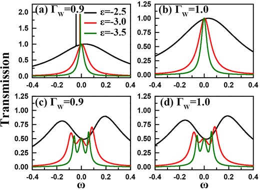
Transmission ability spectra calculated by the SBMFA for different coupling manners between the MBSs and QDs, i.e. (a)–(b) |$\lambda _{j}=0$| and (c)–(d) |$\lambda _{j}=0.5$|⁠. The interchannel coupling |$\Gamma _W$| is (a, c)|$\Gamma _W=0.9$|⁠, and (b, d) |$\Gamma _W=1.0$|⁠, respectively. The parameters are taken to be |$\delta =0$| and |$t_c=0.5$|⁠.

Open in new tabDownload slide

4. Summary

To summarize, in this work we have performed investigations about the electron transport through a double-channel Fano–Anderson structure, by considering the side-coupling of MBSs. As a result, it has been found that in the absence of MBSs, the BIC phenomenon can be induced when interchannel QD–lead couplings are identical to their intrachannel counterparts, manifested as an obviously halved quantum transmission ability. Alternatively, if the balance between the QD–lead couplings is broken, such a BIC will also be destroyed, accompanied by further suppression of the transmission ability. Next, when MBSs are introduced to this system, the BIC phenomenon can be modified efficiently. For the case of two MBSs side-coupled to the QDs in a symmetric way, level degeneracy causes a new additional BIC phenomenon, except for the BIC caused by the QD–lead coupling manner. As only one MBS is incorporated, it suppresses the electron transmission by inducing new transmission dips. When the interdot Coulomb interaction is incorporated, the BIC phenomena are still robust despite the complicated changes of the transmission ability spectra. Based on the obtained results, we can get a basic understanding about the realization of BICs in coupled QDs and their variation in the presence of side-coupled MBSs.

Acknowledgement

This work was financially supported by the LiaoNing Revitalization Talents Program (Grant No. XLYC1907033), the National Natural Science Foundation of China (Grant No. 11905027), the Natural Science Foundation of Liaoning province (Grant No. 2023-MS-072), and Fundamental Research Funds for the Central Universities of Ministry of Education of China (Grant Nos. N2305001, N2209005, and N2205015).

References