Charged Spherical Solution in Torsion and Matter Coupling Gravity and Influence of Torsion Parameter and Electric Charge on Compact Stars in Lower Mass Gap

Author Notes

Abstract

In this study, we explore a new exact solution for a charged spherical model as well as the astrophysical implications of the torsion parameter χ₁ and electric charge Q on compact stars in lower mass gaps in the |$f(\mathcal {T})$| gravity framework. Commencing with the field equations that describe anisotropic matter distributions, we select a well-behaved ansatz for the radial component of the metric function, along with an appropriate formulation for the electric field. The resulting model undergoes rigorous testing to ensure its qualification as a physically viable compact object within the |$f(\mathcal {T})$| gravity background. We extensively investigate two factors: χ₁ and Q, carefully analyzing their impacts on the mass, radius, and stability of the star. Our analyses demonstrate that our models exhibit well-behaved behavior, free from singularities, and can successfully explain the existence of a wide range of observed compact objects. These objects have masses ranging from |$0.85^{+0.15}_{-0.15}$| to 2.67 M_⊙, with the upper value falling within the mass gap regime observed in gravitational events like GW190814. A notable finding of this study has two aspects: we observe significant effects on the maximum mass (M_max) and the corresponding radii of these objects. Increasing values of χ₁ lead to higher M_max (approximately |$2.64^{+0.13}_{-0.14}$|⁠) and smaller radii (approximately |$10.40^{+0.16}_{-0.60}$|⁠), suggesting the possibility of the existence of massive neutron stars within the system. Conversely, increasing values of Q result in a decrease in M_max (approximately |$1.70^{+0.05}_{-0.03}$|⁠) and larger radii (approximately |$13.71^{+0.19}_{-0.20}$|⁠). Furthermore, an intriguing observation arises from comparing the results: for all values of χ₁, nonrotating stars possess higher masses compared to slow-rotating stars, whereas this trend is reversed when adjusting Q.

1. Introduction

Since the early 2000s, the field of altered or enlarged theories of gravity has emerged as a key field of research, with numerous new theories being proposed and extensively investigated. However, the motivation for modifying the underlying theory of general relativity (GR) stretches from the 1920s. Soon after the development of GR, it became clear that the geometric frame upon which the theory is built could be expanded. Furthermore, during that time, progress was made in the endeavor to unify the basic forces through an all-encompassing united field theory, as evidenced by Refs. [1,2].

The early efforts at incorporating geometrical modifications can be collectively examined within the framework of metric-affine systems [3]. These systems typically exhibit invariance under local Lorentz transformations and arbitrary coordinate transformations. When a general affine connection substitutes the Levi-Civita connection, it becomes necessary for the matter action to incorporate this affine connection as well. Consequently, besides the conventional substance input for curvature observed in GR, potential source terms for torsion and nonmetricity also emerge. This phenomenon is evident in the extensively studied Einstein–Cartan theory [4], where it is established that mass relates to curvature while spin relates to torsion, as discussed in Ref. [5]. It is worth noting that matter connections to nonmetricity can provide extra complications [6]. The field equations in these theories are 2nd-order concerning the metric but algebraic for torsion, owing to the specific action that underlies the theory. By requiring 2nd-order field equations from the starting point, the shape of the field equations becomes severely restricted [7]. In these theories, the affine connections, which were previously seen as ancillary to the metric tensor, now play a fundamental and dynamic role. This shift in perspective has given rise to a diverse and expansive landscape of extended and alternative theories of gravity, encompassing a range of formulations and approaches to understanding the gravitational interaction [8–10].

An early notable work on f(R) gravity, possibly discussed by Barrow and Ottewill [11], focused on investigating the stability of cosmological solutions within this framework. However, it took considerably more time for these theories to gain popularity, as indicated by Refs. [9,12,13]. These gravity theories maintain invariance across local transformations like Lorentz and diffeomorphisms, similarly to GR. Nevertheless, they give rise to 4th-order field equations in the measurement, in contrast to the 2nd-order equations in GR. This distinction arises because the Ricci scalar in |$f(R)$| gravity involves second derivatives of the metric. In GR, the higher-order terms involving second derivatives of the metric in the Ricci scalar contribute as a boundary term in the action and do not affect the field equations. However, in |$f(R)$| gravity, these higher-order terms do contribute to the field equations, resulting in 4th-order derivatives in the equations of motion. It is worth noting that decomposing the Ricci scalar into two components, one of which contains only the metric’s first derivatives, yields a theory with 2nd-order field equations. On the other hand, such a theory will probably have extra constraints or drawbacks. Cosmological observations have played a crucial role in constraining various modified gravity models, including |$f(R)$| gravity. According to Clifton et al. [14] and Koyama [15], many of these models have been extensively tested with cosmological data, ensuring a rigorous examination of their validity.

Recently, Astashenok et al. [16] undertook an investigation to explore the maximum mass limit of stars in the framework of|$f(R)$| gravity, specifically in light of the GW190814 event. They selected a causal equation of state (EoS) with a variable speed of sound, incorporating the transition density and pressure corresponding to the SLy EoS. In a recent development, these same authors [17] made a noteworthy discovery using gravitational wave detection, identifying a compact binary coalescence in|$f(R)$| gravity. This discovery unveiled the presence of a compact object with a mass ranging between 2.50 M_⊙ and 2.67 M_⊙. Significantly, this object’s mass places it among either the heaviest NSs ever detected or the lightest black holes (BHs) ever observed. Godzieba et al. [18] adopted a Markov Chain Monte Carlo procedure for generating almost two million phenomenological EoSs, considering both cases with and without 1st-order phase transitions. They focused on fixing the crust EoS and assuming causality at higher densities. They demonstrated how an upper limit on the maximum mass of NSs can be derived from future observations of NS radii and masses. On a different note, Margalit and Metzger [19] combined electromagnetic and gravitational-wave data from the binary NS merger event GW170817 to constrain the radii and maximum mass of NSs. Nathanail et al. [20] used a genetic algorithm to sample the multidimensional parameter space encompassing gravitational-wave and astronomical observations related to GW170817. Their findings align with previous estimates, indicating that all the physical quantities are consistent with the observations when the maximum mass falls within the range of |$M_{\mathrm{ TOV}}=2.210^{+0.116}_{-0.123}~M_{\odot }$| at a 2σ confidence level. In another study, Bombaci et al. [21] explored the prospect that the low-mass partner of the BH in the GW190814 event could be a strange quark star (SQS). This prospect is viable within the framework of the “two-families” scenario, where NSs and SQSs coexist.

Alternatively, one can begin with the teleparallel equivalent of GR (TEGR) [22,23] and explore a range of modified theories of gravity based on torsion [24–31]. While GR and TEGR are equivalent in terms of field equations, their nonlinear extensions diverge, leading to distinct types of modifications. Among these modifications, the simplest is |$f(\mathcal {T})$| gravity, which offers the benefit of 2nd-order derivative field equations. This theory has demonstrated intriguing cosmological applications [32–36] and has been found to align with observational data [37–42]. In our study, we specifically focus on |$f(\mathcal {T})$| gravity for several compelling reasons. Firstly, the Lagrangian of this theory depends solely on the torsion scalar, which makes it comparatively easier to handle than other modified gravitational theories like|$f(R)$| gravity [9,43]. This simplicity in the Lagrangian formulation enhances the tractability and analytical treatment of |$f(\mathcal {T})$| gravity. Secondly, another significant reason for our focus on |$f(\mathcal {T})$| gravity is that its gravitational field equations are of the 2nd order, unlike many other modified theories such as |$f(R)$|,|$f(G)$|⁠, and Born–Infeld modified teleparallelism [10,32,44–50] (see Ref. [10] for a detailed review and comparison of |$f(\mathcal {T})$|⁠, |$f(R)$|⁠, and|$f(G)$|theories). This 2nd-order nature simplifies the analysis and interpretation of the theory’s implications, providing a clearer and more intuitive understanding. However, the primary motivation for modifying the TEGR theory arises from recent observational issues that TEGR alone cannot explain [32]. By introducing the modification of TEGR to |$f(\mathcal {T})$| gravity [51–54], we can potentially address these unresolved issues. Notably, employing |$f(\mathcal {T})$| gravity allows for explanations not only of inflation in the early universe [32] but also of the observed late-time cosmic acceleration [55–58]. Furthermore, |$f(\mathcal {T})$| gravity exhibits a wide range of viable applications, making it an intriguing choice for our investigation. It has been extensively employed in the realm of cosmology, offering insights and solutions to various cosmological phenomena [38,59–61]. Additionally, |$f(\mathcal {T})$| gravity has found interesting applications in the field of astrophysics, contributing to our understanding of gravitational phenomena and astrophysical objects [62–66]. Moreover, an exciting breakthrough in gravitational physics was made by Junior et al. [67], who discovered a novel class of exact regular BH solutions incorporating nonlinear electrodynamics. Hussain et al. [68] employed conformal vector fields within gravity to identify static spherically symmetric perfect fluid spacetimes. In contrast, Zhao et al. [69] focused their investigation on the quasinormal mode frequencies of a test massless scalar field and an electromagnetic field within the context of gravity. Their approach involved extracting spherically symmetric solutions via perturbative techniques and utilizing two metric function ansatzes to quantify deviations from the Schwarzschild solution. Subsequently, their focus shifted towards quadratic modifications, which are considered a suitable approximation for realistic theories. Junior et al. [67] delved into the formulation of black-bounce spacetime solutions in four dimensions within the framework of gravity. They began by introducing the case of the diagonal tetrad, which was then subdivided into scenarios involving zero torsion, constant torsion, and teleparallel equations of motion. In their work, DeBenedictis et al. [70] focused on the examination of the fundamental properties of the vacuum within the framework of TEGR. They introduced a quadratic torsion term into the action to further explore and analyze the essential characteristics.

Within the domain of |$f(\mathcal {T})$| gravity theory, Houndjo et al. [71] delved into the investigation of two intriguing cosmological models distinguished by distinct formulations of the Hubble parameter. Their work achieved the unification of the early-time and late-time acceleration eras with the radiation- and matter-dominated eras. In an intriguing approach, Golovnev and Guzmán [72] examined the properties of static spherically symmetric solutions in gravity. They showcased a simplification in the search for solutions by employing two relatively straightforward equations, building upon their prior work on generalizing Bianchi’s identities within this theory. On a different note, Nashed and Saridakis [73] utilized a perturbative technique to explore the stability of motion and thermodynamics in the context of spherically symmetric solutions within gravity. Their investigation shed light on the dynamics and thermodynamic aspects of these solutions. They extracted charged BH solutions with and without perturbative corrections in the charge distribution, accounting for slight deviations from GR. In their study, Hu et al. [74] investigated the scalar perturbations and potential strong coupling issues of |$f(\mathcal {T})$| theory within a cosmological background using the effective field theory approach. Ren et al. [75] focused on covariant gravity and determined the deflection angle, positions, and magnifications of lensed images. Using a weak-field, perturbative approximation, they analyzed deviations from the solutions from GR. De Araujo and Fortes [76] analyzed a gravity model incorporating torsion and its application to compact objects such as neutron stars (NSs). They investigated the effects of this model on NSs by considering various EoSs. The effects of the modification on the properties of nonrotating NSs were investigated by Lin et al. [77]. They utilized the SLy and BSk families of EoSs to describe the matter inside NSs and examined how the modification affected the NS models. Debnath [78] focused on the charged gravastar model within a four-dimensional, spherically symmetric stellar system. By incorporating modified gravity theory and an electromagnetic field, the study examined the properties and characteristics of these gravastars as an alternative to BHs. In a novel approach, Das et al. [79] introduced the concept of gravastars as an alternative stellar model in the context of modified gravity based on the Mazur–Mottola postulate. This model offered a unique perspective on the nature of compact objects and their gravitational behavior. Additionally, Zubair and Abbas [80] proposed analytical models for anisotropic strange stars within the framework of modified gravity. Their investigation utilized an off-diagonal tetrad and provided valuable insights into the properties and structure of these intriguing astrophysical objects. Bhar et al. [81] successfully derived analytically relativistic quintessence anisotropic spherical solutions within the |$f(\mathcal {T})$| paradigm. This was achieved through the utilization of a pressure anisotropy condition and a metric potential of the Tolman–Kuchowicz type. In a recent research endeavor, Maurya, Errehymy, and their colleagues [82] successfully derived an anisotropic solution for static and spherically symmetric configurations within the |$f(\mathcal {T})$| gravity theory. This accomplishment entailed demanding the vanishing of the complexity factor and employing the isotropization approach via the gravitational decoupling method. In a recent study [83], the author focused on examining the spherically symmetric and static self-gravitating structures of anisotropic fluids within the context of the torsion-dependent extended theory of gravity. The investigation involved assuming a linear EoS and utilizing the Tolman–Kuchowicz ansatz for the metric functions, taking into account the effects of gravity. There exist several earlier works in the literature that discuss compact objects in modified gravity, with notable contributions from Refs. [84–88]. Moreover, Refs. [89,90] offer valuable insights into cosmological observational constraints in this context. Recently, Baskey et al. [91,92] investigated new exact solutions for anisotropic matter distribution in GR by choosing a specific form of anisotropy.

One compelling motivation for considering |$f(\mathcal {T})$| gravity as a more realistic framework for modeling stars, despite the success of |$f(R)$| gravity in explaining inflation and dark energy, lies in the unique features and implications of |$f(\mathcal {T})$| gravity specifically related to compact objects. |$f(\mathcal {T})$| gravity incorporates torsion, a geometric quantity associated with the intrinsic angular momentum of matter, which introduces additional effects and interactions. This inclusion of torsion allows |$f(\mathcal {T})$| gravity to capture the intricate dynamics and behavior of highly dense and strongly gravitating objects like stars more accurately. The modified field equations of |$f(\mathcal {T})$| gravity, compared to f(R) gravity, may lead to different predictions for the structure, stability, and mass–radius relation of stars. By focusing on |$f(\mathcal {T})$| gravity, researchers can explore the specific torsion-related effects that play a crucial role in the behavior of stars, providing a more comprehensive and realistic description. Furthermore, the consistency of |$f(\mathcal {T})$| gravity with relevant observational data and its theoretical coherence, including its mathematical simplicity and foundational aspects, further strengthen the argument for its suitability in modeling stars. Different applications have been investigated in these modified theories of gravity with torsion. The existence of relativistic stars was first investigated in Ref. [93]. Compact stars in a specific |$f(\mathcal {T})$| model for an isotropic fluid with a polytropic EoS were presented in Ref. [94], and later the authors extended the analysis to boson stars [95]. These studies demonstrate the broad range of applications and the potential of |$f(\mathcal {T})$| gravity in understanding the properties and behavior of compact stellar objects. Based on the aforementioned arguments, we have been motivated to introduce a novel exact solution for a charged spherical model within the framework of |$f(\mathcal {T})$| gravity in this paper. Our proposed solution is obtained by solving the field equation, employing a well-behaved ansatz for the radial component of the metric function, and employing an appropriate form of the electric field.

The structure of the current paper is as follows. In Sect. 2, we provide a concise overview of the field equations in |$f(\mathcal {T})$| gravity and introduce the unique solution that describes the charged stellar configuration. Section 3 addresses the expressions for the model parameter, which are derived from the smooth matching conditions at the stellar surface. The physical analysis of the resulting model is discussed in Sect. 4, while the stability analysis is presented in Sect. 5. In Sect. 6, we delve into the characteristics of the mass–radius relation and compactness of different compact objects via M–R curves while moment of inertia is discussed in Sect. 7. Finally, we provide concluding remarks in Sect. 8.

2. Static spherical symmetry field equation in T gravity

The gravity theory under the electromagnetic field is derived from the action expressed as

$$\begin{eqnarray} S=\int \left [ \frac{1}{16\pi } f(\mathcal {T})+\mathcal {L}_{\mathrm{ Matter}}+ \mathcal {L}_{E}\right] dx^{4}\, e. \end{eqnarray}$$

(1)

In the context of natural (geometrized) units where G = c = 1, the variable f denotes a function that relies on the torsion scalar |$\mathcal {T}$|⁠, whereas |$\mathcal {L}_{\mathrm{ Matter}}$| and |$\mathcal {L}_{e}$| represent the Lagrangian density for matter field and electromagnetic field, respectively. Let us write a general line element of a manifold,

$$\begin{eqnarray} ds^{2}=g_{\eta \sigma }dx^{\eta }dx^{\sigma }=\eta _{u l}h_{\eta }^{u}\theta _{\sigma }^{l}dx^{\eta }dx^{\sigma } . \end{eqnarray}$$

(2)

Here we denote: η_ul = diag[1, −1, −1, −1], |$dx^{\eta }=e_{u}^{\eta }h^{u}$|⁠, |$h^{u}=e_{\eta }^{u}dx^{\eta }$|⁠. In this context, Greek symbols are used to represent spacetime indices, whereas Latin symbols are used for tetrad indices. Also, the value of e is |$e=\sqrt{-g}=\mathrm{ det}[e^{\eta }_{\sigma }]$|⁠. As long as the Riemann tensor is not zero and the torsion acts as a nonzero, it is possible to express the Weitzenbock antisymmetric connections,

$$\begin{eqnarray} \Gamma _{\sigma \eta }^{\sigma }&=&e^{\sigma }_{u}\partial _{\alpha }e^{u}_{\beta } . \end{eqnarray}$$

(3)

The expressions that are used to denote the torsion and contorsion tensors are as follows:

$$\begin{eqnarray} \mathcal {T}_{~\sigma \eta }^{\sigma }&=&\Gamma _{~\sigma \eta }^{\sigma } - \Gamma _{~ \eta \sigma }^{\sigma }=e^{\sigma }_{\eta }\left(\partial _{\alpha }e^{\eta }_{~\beta }-\partial _{\beta }e^{\eta }_{~\alpha }\right), \end{eqnarray}$$

(4)

$$\begin{eqnarray} K^{\sigma }_{~\sigma \eta }&=&-\frac{1}{2}\left(\mathcal {T}^{\sigma }_{\alpha \beta }-\mathcal {T}^{~\sigma }_{\alpha ~\beta }-\mathcal {T}^{~\sigma }_{ \beta ~\alpha }\right). \end{eqnarray}$$

(5)

The two tensors that were discussed before, Eqs. (4) and (5), are combined in order to produce a new tensor, which is now referred to as

$$\begin{eqnarray} S^{~\sigma \eta }_{\sigma }&=&\frac{1}{2}\left(\delta ^{\alpha }_{\sigma }\mathcal {T}^{n \beta }_{n}+K^{\sigma \eta }_{\sigma }-\delta ^{\beta }_{\sigma } \mathcal {T}^{n \alpha }_{n} \right). \end{eqnarray}$$

(6)

A possible representation of the torsion scalar is given by the following expression:

$$\begin{eqnarray} \mathcal {T}&=&\mathcal {T}_{\sigma \eta }^{\sigma } S^{\sigma \eta }_{\sigma }. \end{eqnarray}$$

(7)

In order to derive the system of equations governing the motion, Eq. (1) is varied against the tetrad field,

$$\begin{eqnarray} e_{\alpha }^{\eta }S_{\eta }^{\beta \sigma }\partial _{\alpha }\mathcal {T}f_{\mathcal {T}\mathcal {T}}+e^{-1}\left(ee_{\alpha }^{\eta }S_{\eta }^{\beta \sigma }\right)f_{\mathcal {T}}+e_{\alpha }^{\beta }\mathcal {T}_{\beta \epsilon }^{\eta }S_{\eta }^{\sigma \epsilon }f_{\mathcal {T}} - \frac{1}{4}e_{\alpha }^{\sigma }f =-4\pi e_{\alpha }^{\eta } \left (T_{\eta }^{\sigma } +E_{\eta }^{\sigma }\right ).~~ \end{eqnarray}$$

(8)

The Lagrangian density |$\mathcal {L}_{\mathrm{ matter}}$| is symbolized by the tensor |$T^\sigma _\eta$|⁠, which is the stress-energy tensor. However, |$E_{\eta }^{\sigma }$| represents the tensor for |$\mathcal {L}_E$| which is responsible for the electromagnetic field. Nevertheless, the symbols |$f_{\mathcal {T}}$| and |$f_{\mathcal {TT}}$| are denoted as |$f_{\mathcal {T}}=\frac{\partial f}{\partial \mathcal {T}}$| and |$f_{\mathcal {T}\mathcal {T}}=\frac{\partial ^{2} f}{\partial \mathcal {T}^2}$|⁠. The stress-energy tensor is defined as follows under the assumption of an isotropic fluid distribution:

$$\begin{eqnarray} T_{\sigma }^{\eta }=(\rho +P)L_{\sigma }L^{\eta }-P\delta _{\sigma }^{\eta }. \end{eqnarray}$$

(9)

In this context, the 4-speed-vector can be expressed by the equation |$L_{\sigma }=e^{\eta }\delta _{\sigma }^{0}$| . The symbols P and ρ indicate the pressure and energy density, respectively.

In the field of |$f(\mathcal {T})$| gravity, the equation of motion may be stated in a different form by using the covariant derivative formalism,

$$\begin{eqnarray} G_{\sigma \eta }f_{\mathcal {T}}+S_{\eta \sigma }^{\alpha }\nabla _{\alpha }\mathcal {T}f_{\mathcal {T}\mathcal {T}}+\frac{\mathcal {T}}{2}\left(\frac{f}{\mathcal {T}}-f_{\mathcal {T}}\right)g_{\sigma \eta } =\frac{1}{16\pi } \left (T_{\sigma \eta } +E_{\sigma \eta } \right ). \end{eqnarray}$$

(10)

The Einstein tensor is represented by the symbol G_ση. Equation (8) may be reformulated using the principles of GR and the |$f(R)$| field equations in the following manner:

$$\begin{eqnarray} G_{\sigma \eta }=\frac{1}{16\pi f_{\mathcal {T}}}\left(T_{\sigma \eta }+\mathcal {T}_{\sigma \eta }^{[\mathcal {T}]}\right). \end{eqnarray}$$

(11)

The term torsion tensor |$\mathcal {T}_{\sigma \eta }^{[\mathcal {T}]}$| incorporates modifications that are obtained from the torsion scalar,

$$\begin{eqnarray} \mathcal {T}_{\sigma \eta }^{^{[\mathcal {T}]}}=\frac{-1}{64\pi }\left (4S_{\eta \sigma }^{\alpha }\nabla _{\alpha }f_{\mathcal {T}\mathcal {T}}+\left(\mathcal {R}f_{\mathcal {T}}-S_{\eta \sigma \eta }^{\alpha }\nabla _{\alpha }f_{\mathcal {T}\mathcal {T}}+\mathcal {T}\right) g_{\sigma \eta }\right ). \end{eqnarray}$$

(12)

Equation (10) clearly produces the equations of GR for a linear function |$f(\mathcal {T})$|⁠, more precisely when |$f(\mathcal {T})$| is equal to |$\mathcal {T}$|⁠.

Following that, we are going to concentrate on the internal composition of the spherically symmetrical and static fluid distribution, which is defined as:

$$\begin{eqnarray} ds^2 &=& e^{\varphi (r)}dt^{2}-e^{\tau (r) }dr^{2}-r^{2} d \theta ^{2}-r^{2}\sin ^{2} \theta ~d \Omega ^{2}.~~~ \end{eqnarray}$$

(13)

The characters φ(r) and τ(r) stand for the two gravitational potentials that rely only on the radial coordinate, r. Furthermore, we construct the stress-energy tensor for a self-gravitating system with isotropic distribution in 3D space using the following formula:

$$\begin{eqnarray} T_{\eta }^{\sigma }=\mathrm{ diag} \left( \rho , -P, -P, -P \right), \end{eqnarray}$$

(14)

with

$$\begin{eqnarray} T_{\eta }^{\sigma }=0 , \ \ \mathrm{ if}\ \eta \ne \sigma . \end{eqnarray}$$

(15)

The metric potentials φ and τ are responsible for determining the value of the pressure and density. Moreover, the electromagnetic field tensor may be described as follows:

$$\begin{eqnarray} E_{\eta \sigma }=\frac{1}{4\pi } \left(-F^{\alpha }_{\eta }F_{\sigma \, \alpha } + \frac{1}{4}{g_{\eta \sigma }} F_{\beta \, \alpha }F^{\beta \, \alpha } \right). \end{eqnarray}$$

(16)

This equation describes the electromagnetic field tensor F_ησ, which is antisymmetric. Furthermore, it is important to mention that the nonzero elements of the electromagnetic field tensor, namely F⁰¹ and F¹⁰, correspond to the radial element of the electric field. The mathematical expression that represents the link between these two components is F⁰¹ = −F¹⁰. The connection between electric field (E) and these tensor components F⁰¹ and F⁰¹ along with the metric functions τ(r) and φ(r) may be expressed as,

$$\begin{eqnarray} F^{01} = - F^{10}=E \, e^{-(\tau +\varphi )/2}. \end{eqnarray}$$

(17)

Given the relativistic Gauss-law and the associated electric field E, the quantity q(r), which denotes an electric charge for the spherical system with radial coordinates r, can be given as

$$\begin{eqnarray} \mathrm{ q}(r)=\frac{1}{2}\int ^{r}_{0}{\sigma \, r^2\, e^{\lambda /2} dr}=r^2\, \sqrt{-F_{10}\, F^{10}} \end{eqnarray}$$

(18)

$$\begin{eqnarray} E^2=-F_{10}\, F^{10}=\frac{q^2}{r^4}. \end{eqnarray}$$

(19)

On the other hand, in Eq. (9), the tetrad matrix for the line element is represented by the following equation:

$$\begin{eqnarray} \left [e^{\sigma }_{\eta }\right ]=\mathrm{ diag}\left [e^{\varphi /2 },~e^{\tau /2},~r,~r\sin \theta \right ] . \end{eqnarray}$$

(20)

Conversely, the determinant of this tensor may be expressed as

$$\begin{eqnarray} e=\mathrm{ det}\left [e^{n}_{u}\right ]=e^{(\varphi +\tau )/2}\, r^2\sin \theta . \end{eqnarray}$$

(21)

Within the context of the radial coordinate r, the torsion scalar, together with its derivative, can be defined as

$$\begin{eqnarray} \mathcal {T}(r)=\frac{2 e^{-\tau }}{r^2} \left [r\, \varphi ^{\prime }+1\right ], \end{eqnarray}$$

(22)

$$\begin{eqnarray} \mathcal {T}^{\prime }(r)=\frac{e^{-\tau }}{r} \left [\varphi ^{\prime \prime }-\frac{1}{r^2}-\left(\varphi ^{\prime }+\frac{1}{r}\right)\left(\tau ^{\prime }+\frac{1}{r}\right)\right ].~ \end{eqnarray}$$

(23)

The prime sign (′) represents the derivative in terms of radial coordinates. It is possible to explicitly construct the equations of motion for an anisotropic fluid under |$f(\mathcal {T})$| gravity by replacing the tetrad field that was described before under Eq. (20) and entering the torsion scalar and its derivative into Eq. (8) as

$$\begin{eqnarray} 8\pi \rho &=& f_\mathcal {T} \left [\frac{1}{r^2}+\frac{1}{r}e^{-\tau } \left(\tau ^{\prime }+\varphi ^{\prime }\right)-\mathcal {T}(r)\right ]+\frac{f}{2}-\frac{q^2}{r^4},~~ \end{eqnarray}$$

(24)

$$\begin{eqnarray} 8\pi P &=& f_\mathcal {T} \left [-\frac{1}{r^2}+\mathcal {T}(r)\right ]-\frac{f}{2}+\frac{q^2}{r^4}, \end{eqnarray}$$

(25)

$$\begin{eqnarray} 8\pi P &=&f_\mathcal {T} \left [e^{-\tau } \left(\left(\frac{\varphi ^{\prime }}{4}+\frac{1}{2 r}\right) \left(\varphi ^{\prime }-\tau ^{\prime }\right)+\frac{\varphi ^{\prime \prime }}{2}\right)+\frac{\mathcal {T}(r)}{2}\right ]-\frac{f}{2}-\frac{q^2}{r^4}. \end{eqnarray}$$

(26)

When considering the concept of |$f(\mathcal {T})$| gravity, it turns out to be achievable to get an extra off-diagonal quantity as

$$\begin{eqnarray} \frac{\mathrm{ cot}\theta }{2r^2} \mathcal {T}^{\prime } f_{\mathcal {T}\mathcal {T}}=0. \end{eqnarray}$$

(27)

This is not the same situation as what happens in GR. Two types of choices can be deduced from Eq. (27): (a) |$\mathcal {T}^{\prime }=0$|⁠, and (b) |$f_{\mathcal {T}\mathcal {T}}=0$|⁠. The first scenario does not provide the exact Schwarzschild de-Sitter spacetime. Therefore, we must discard this case. Therefore, the second scenario has the following linear functional form:

$$\begin{eqnarray} f_{\mathcal {T}\mathcal {T}}=0~~\rightarrow ~~ f(\mathcal {T})=\chi _1 \mathcal {T} + \chi _2. \end{eqnarray}$$

(28)

The parameters α and γ represent integration constants. Through the process of incorporating Eq. (28) into the field equations (24)–(26), we are able to reach the final field equations,

$$\begin{eqnarray} \rho = \frac{1}{16 \pi r^2}[2\chi _1 + 2e^{-\tau }\chi _1(r\tau ^{\prime }-1)-r^2\chi _2]-\frac{q^2}{8\pi r^4}, \end{eqnarray}$$

(29)

$$\begin{eqnarray} P= \frac{1}{16 \pi r^2}[-2\chi _1+2e^{-\tau }\chi _1(r\varphi ^{\prime }+1)+r^2\chi _2]+\frac{q^2}{8\pi r^4}, \end{eqnarray}$$

(30)

$$\begin{eqnarray} P = \frac{e^{-\tau }}{32 \pi r}[2e^{\tau }r\chi _2+\chi _1(2+r\varphi ^{\prime })(\varphi ^{\prime }-\tau ^{\prime })+2r\chi _1\varphi ^{\prime \prime }]-\frac{q^2}{8\pi r^4}.~~ \end{eqnarray}$$

(31)

Furthermore, we find the pressure isotropic condition by subtracting Eqs. (30) and (31) as,

$$\begin{eqnarray} \chi _1\, e^{-\tau }\left [ (2 \varphi ^{\prime \prime }+ \varphi ^{\prime 2}) r^2-2 \varphi ^{\prime } r- \tau ^{\prime } r ( \varphi ^{\prime }r+2)+4 (e^{\tau }-1)\right ] =8 r^2 E^2.~~~~~ \end{eqnarray}$$

(32)

For the differential equation to be solved, it is required to have three conditions. This is because the pressure isotropic equation (32) has four unknowns, which means that the equation cannot be solved without these conditions. Taking into consideration this particular reason, we choose a physically feasible ansatz for the potential τ(r) of the form,

$$\begin{eqnarray} \tau (r)=\ln \left [\frac{1-2\gamma r^2}{1+\gamma r^2} \right ], \end{eqnarray}$$

(33)

where γ is a constant with dimension l⁻². It is worth mentioning that Baskey et al. [91] have already used the metric function (33) in the context of GR.

By plugging Eq. (33) into Eq. (32), we get

$$\begin{eqnarray} &&2 r \left(1-2 \gamma ^2 r^4-\gamma r^2\right) \varphi ^{\prime \prime } +\left (r-2 \gamma ^2 r^5-\gamma r^3\right )\varphi ^{\prime 2} +\left (4 \gamma ^2 r^4 + 8 \gamma r^2-2\right ) \varphi ^{\prime }\\ &&\quad=\frac{8 q^2 \left(1-2 \gamma r^2\right)^2-24\chi _1 \gamma ^2 r^6}{\chi _1\, r^3}. \end{eqnarray}$$

(34)

The solution of the above differential equation depends on the suitable expression for the electric charge q(r). It is mentioned that we choose the following expression of electric charge q(r):

$$\begin{eqnarray} \mathrm{ q}(r)=\sqrt{\frac{3 \chi _1 \gamma ^2 r^6}{ (1-2\gamma r^2)^2}}. \end{eqnarray}$$

(35)

Equation (35) demonstrates that q(r) is zero at the core r = 0 and afterward grows as r rises. By replacing the value of q(r) in Eq. (34), we derive

$$\begin{eqnarray} \varphi ^{\prime \prime } -\varphi ^{\prime 2} \frac{\left(1-2 \gamma ^2 r^4-\gamma r^2\right)}{2 \left(2 \gamma ^2 r^4+\gamma r^2-1\right)}-\varphi ^{\prime } \frac{\left(4 \gamma ^2 r^4+8 \gamma r^2-2\right) }{ 2 r \left(2 \gamma ^2 r^4+\gamma r^2-1\right)}=0. \end{eqnarray}$$

(36)

Now we use the transformation φ = 2ln Ψ to convert the differential equation (36) in its simplest form as,

$$\begin{eqnarray} \Psi ^{\prime \prime } r \left(2 \gamma ^2 r^4+\gamma r^2-1\right)-\Psi ^{\prime } \left(2 \gamma ^2 r^4+4 \gamma r^2-1\right)=0. \end{eqnarray}$$

(37)

Upon solving the aforementioned differential equation (37), the following solution is obtained:

$$\begin{eqnarray} \Psi (r)&=&\frac{A}{2 \gamma } \Biggr (\sqrt{1-\gamma r^2-2\gamma ^2r^4}-\frac{9 \tan ^{-1}\left(\frac{\sqrt{6}-2 \sqrt{\gamma r^2+1}}{\sqrt{2-4 \gamma r^2}}\right)}{\big(\sqrt{6 \gamma r^2+6}-3\big)^2} \\ &&\times \left(2 \sqrt{2} \gamma r^2-4 \sqrt{3 \gamma r^2+3}+5 \sqrt{2}\right)\Biggr )+B. \end{eqnarray}$$

(38)

Then the expressions for density and pressure are given as,

$$\begin{eqnarray} 8\pi \rho = \frac{3 \gamma \chi _1 \left(\gamma r^2-3\right)}{\left(1-2 \gamma r^2\right)^2}-\frac{\chi _2}{2}, \end{eqnarray}$$

(39)

$$\begin{eqnarray} 8\pi P = \gamma \chi _1 \left(\frac{4 A \sqrt{\gamma r^2+1}}{\sqrt{1-2 \gamma r^2} \mathrm{ P}_{1}(r)}+\frac{3 \gamma r^2}{\left(1-2 \gamma r^2\right)^2}+\frac{3}{1-2 \gamma r^2}\right)+\frac{\chi _2}{2}, \end{eqnarray}$$

(40)

where,

$$\begin{eqnarray} \mathrm{ P}_1(r)=-3 \sqrt{2} A \tan ^{-1}\left(\frac{\sqrt{6}-2 \sqrt{\gamma r^2+1}}{\sqrt{2-4 \gamma r^2}}\right)+2 B \gamma +A \sqrt{\gamma r^2+1} \sqrt{1-2 \gamma r^2}. \end{eqnarray}$$

3. Boundary conditions

Considering the linear functional form of the |$f(\mathcal {T})$| gravity theory within the framework of charged matter distribution, it is possible that the exterior Reissner–Nordström de-Sitter solution is the most appropriate external spacetime solution:

$$\begin{eqnarray} ds^2 = \bigg (1-\frac{2{M}}{r}+\frac{Q^2}{r^2}-{\Lambda \over 3}~r^2\bigg ) dt^2- \frac{dr^2}{\bigg (1-\frac{2{M}}{r}+\frac{Q^2}{r^2}-{\Lambda \over 3}~r^2\bigg )} - r^2 (d\theta ^2 + \sin ^2\theta d\phi ^2). \end{eqnarray}$$

(41)

Let M and Q denote the aggregate mass and charge of the stellar object at the surface r = R and |$M=m(r_{_\Sigma })/\chi _1$|⁠. Furthermore, the value of Λ is equivalent to χ₂/2χ₁. Moreover, the use of the first and second fundamental forms produces the subsequent results:

$$\begin{eqnarray} \bigg (1-\frac{2{{M}}}{R}+\frac{Q^2}{R^2}-{\Lambda \over 3}~R^2\bigg )&=&e^{\varphi (R)},~~~ \end{eqnarray}$$

(42)

$$\begin{eqnarray} \bigg (1-\frac{2{{M}}}{R}+\frac{Q^2}{R^2}-{\Lambda \over 3}~R^2\bigg )&=&e^{-\tau (R)},~~~ \end{eqnarray}$$

(43)

$$\begin{eqnarray} \mathrm{ P}(R)&=&0.~~~ \end{eqnarray}$$

(44)

At the surface r = R, the boundary conditions that have been discussed above are the ones that are most suitable for the joining of two spacetimes simultaneously. Utilizing Eqs. (42)–(44), we can determine the constants A, B, and M as,

$$\begin{eqnarray} A &=& \Big [2 \gamma \sqrt{\gamma R^2+1} \left(\sqrt{6 \gamma R^2+6}-3\right)^2\Big ]\Big /\Biggr [\sqrt{1-2 \gamma R^2} \Biggr \lbrace \left(\sqrt{6 \gamma R^2+6}-3\right)^2\\ &&\times \big (\sqrt{\gamma R^2+1} \sqrt{1-2 \gamma R^2} + 2 \gamma \zeta _1(R) \big )-9 \left(2 \sqrt{2} \gamma R^2-4 \sqrt{3 \gamma R^2+3}+5 \sqrt{2}\right)\\ &&\times \tan ^{-1}\left(\frac{\sqrt{6}-2 \sqrt{\gamma R^2+1}}{\sqrt{2-4 \gamma R^2}}\right)\Biggr \rbrace \Biggr ], \end{eqnarray}$$

(45)

$$\begin{eqnarray} B &=& \zeta _1(R) \, \Big [2 \gamma \sqrt{\gamma R^2+1} \left(\sqrt{6 \gamma R^2+6}-3\right)^2\Big ]\Big /\Biggr [\sqrt{1-2 \gamma R^2} \Biggr \lbrace \left(\sqrt{6 \gamma R^2+6}-3\right)^2 \\ &&\times \,\,\big (\sqrt{\gamma R^2+1} \sqrt{1-2 \gamma R^2} +2 \gamma \zeta _1(R) \big )-9 \left(2 \sqrt{2} \gamma R^2-4 \sqrt{3 \gamma R^2+3}+5 \sqrt{2}\right) \\ &&\times \,\,\tan ^{-1}\left(\frac{\sqrt{6}-2 \sqrt{\gamma R^2+1}}{\sqrt{2-4 \gamma R^2}}\right)\Biggr \rbrace \Biggr ], \end{eqnarray}$$

(46)

$$\begin{eqnarray} M=\frac{1}{12} R^3 \left(\frac{18 \gamma \left(\gamma R^2 \chi _1+2 \gamma R^2-1\right)}{\left(1-2 \gamma R^2\right)^2}-\frac{\chi _2}{\chi _1}\right), \end{eqnarray}$$

(47)

where,

$$\begin{eqnarray} \zeta _1(R) &=& \Bigg [\chi _2 \left(1-2 \gamma R^2\right)^2 \Bigg (\left(2 \gamma R^2-1\right) \sqrt{\gamma R^2+1}+3 \sqrt{2-4 \gamma R^2} \tan ^{-1}\left(\frac{\sqrt{6}-2 \sqrt{\gamma R^2+1}}{\sqrt{2-4 \gamma R^2}}\right)\Bigg ) \\ &&-\,\,2 \gamma \chi _1 \Bigg (9 \left(\gamma R^2-1\right) \sqrt{2-4 \gamma R^2} \tan ^{-1}\left(\frac{\sqrt{6}-2 \sqrt{\gamma R^2+1}}{\sqrt{2-4 \gamma R^2}}\right) +(22 \gamma ^2 R^4-25 \gamma R^2+7) \\ &&\times \,\, \sqrt{\gamma R^2+1}\Bigg )\Bigg ] \Big / \Big [2 \gamma \sqrt{1-2 \gamma R^2} \big \lbrace \chi _2 \left(1-2 \gamma R^2\right)^2-6 \gamma \chi _1 \left(\gamma R^2-1\right)\big \rbrace \Big ]. \end{eqnarray}$$

4. Physical analysis

To provide an accurate explanation of charged anisotropic compact stars, we are going to look at how the model’s structural physical characteristics shift based on the physical conditions.

Our initial focus is on examining the regularity of the metric coefficients in the context of studying relativistic compact configurations. Singularities pose a significant challenge in this field of research. To ensure the physical feasibility of the solutions, it is crucial for the metric coefficients in charged compact stars to be both regular and positive. As stated in Ref. [96], the expected form and physical tractability of the solutions are ensured by the metric coefficients in Eq. (33) for τ(r) and Eq. (38) for φ(r), particularly in the vicinity of the stellar core. Hence, the metric coefficients being examined exhibit regularity, demonstrate a smooth behavior, and remain free from any central singularity within the interior of the stellar object.

Moreover, it is common knowledge that the existence of a positive electric charge within a self-gravitating charged fluid compact object results in a repulsive force that prevents gravitational collapse [97,98]. By introducing the electric field into the stellar structure, we can effectively avoid the formation of singularities. Additionally, this repulsive electric force, arising from the positive electric charge, plays a crucial role in maintaining equilibrium and counteracting gravitational collapse. According to Fig. 1, the electric charge starts at zero at the core and grows as we move towards the boundary of the star for all values of χ₁. The maximum charge is attained when χ₁ equals 0.45. This characteristic behavior of the electric charge indicates that the electric force produced by the charge operates outwardly within the interior of the stars. According to the findings of Treves and Turolla [99], Ray and Das [100,101] provide an argument for the current study involving a charged fluid distribution. They claim that while most astrophysical structures are electrically neutral, recent research does not dismiss the possibility of the presence of massive astrophysical structures that lack electrical neutrality. The procedure primarily involves the acquisition of an overall electric charge via the process of accretion from the surrounding medium or possibly from a compact object during its collapse from the supernova stage. It is noteworthy that the investigation of electric charge’s impact on compact structures is of relevance in this context. Ray et al. [102] have shown that a significant impact on the behavior of compact stars can be observed if the total electric charge is around 10²⁰C. In the present study, we have calculated the following amount of charge on a compact star for different torsion parameters χ₁ with fixed χ₂ = −0.0024: (i) 2.35199 × 10²⁰C for χ₁ = 0.30, (ii) 2.54044 × 10²⁰C for χ₁ = 0.35, (iii) 2.71584 × 10²⁰C for χ₁ = 0.40, and (iv) 2.88058 × 10²⁰C for χ₁ = 0.45.

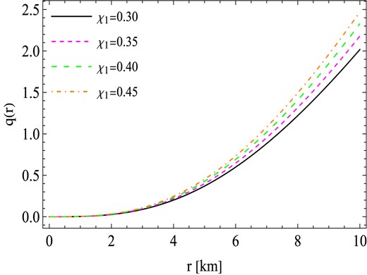
The behavior of electric charge q(r) against the radial coordinates r for the values of free parameters γ = −0.0037 km−2, R = 10 km, and χ2 = −0.0024 km−2.

Fig. 1.

The behavior of electric charge q(r) against the radial coordinates r for the values of free parameters γ = −0.0037 km⁻², R = 10 km, and χ₂ = −0.0024 km⁻².

Open in new tab Download slide

Proceeding further, the determination of the equilibrium gravitational mass attainable at a stable radius within a star is significantly influenced by the energy density, which plays a pivotal role in this determination. In the case of compact stars that are gravitationally confined and charged, it is expected that the energy density is highest at the core and progressively diminishes towards the surface. The behavior of the energy density, denoted as ρ(r), is visually represented in Fig. 2. It is noteworthy that the energy density reaches its maximum at the center and gradually decreases as the radius r increases. Eventually, it reaches a minimum at the surface for each parameter branch defined as χ₁ ∈ [0.3, 0.45]. It is worth noting that the parameter χ₁ facilitates the gravitational condensation of matter at lower densities. An increase in χ₁ causes ρ(r) to shift towards lower equilibrium values throughout the interior of the star, specifically where r is less than the radius R.

Fig. 2.

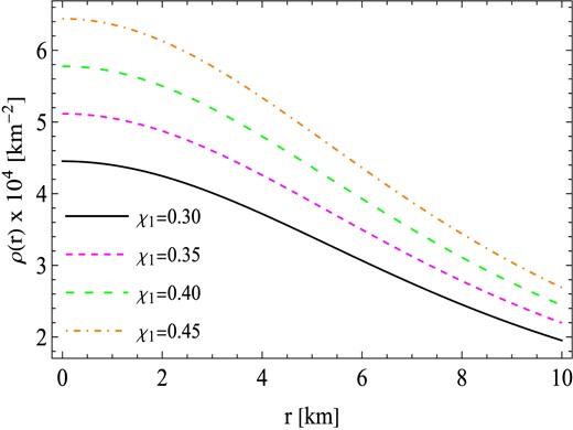
The behavior of density ρ(r) against the radial coordinates r with similar values of constants to those used in Fig. 1.

Open in new tab Download slide

In the case of compact stars, regardless of their charge, it is expected that the inner pressures reach their maximum and finite values at the center. Importantly, in our scenario, the radial component of the pressure, which is equivalent to the tangential component, vanishes at the surface. The behavior of this pressure is depicted in Fig. 3. Notably, for each parameter branch defined as χ₁ ∈ [0.3, 0.45], it is intriguing to observe that the pressure remains finite throughout the interior of the star. The highest pressure values are located at the center and gradually decrease towards the stellar surface, where the lowest pressure values are observed.

Fig. 3.

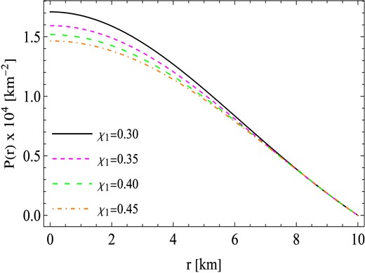
The behavior of pressure P(r) against the radial coordinates r with similar values of constants to those used in Fig. 1.

Open in new tab Download slide

In the study of compact structures within classical GR and modified theories of gravitation, the EoS plays a crucial role. It provides valuable insights into the composition of matter within the star. The barotropic EoS expressed as p = p(ρ), where p represents pressure and ρ denotes density, offers significant indications about the nature of the stellar matter. Figure 4 presents an illuminating analysis of the relationship between the ratio of pressure to density, p(r)/ρ(r), and the radial coordinate, r. Notably, our findings reveal that the pressure remains consistently lower than the density at every interior point of the compact object. Moreover, the ratio p/ρ is observed to be positive throughout the entire interior region of the star for each parameter branch, χ₁ ∈ [0.3, 0.45]. These observations deepen our understanding of the compact object’s properties, shedding light on the interplay between the EoS and the physical characteristics of the system.

Fig. 4.

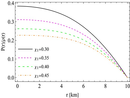
The behavior of pressure and density ratio (P(r)/ρ(r)) against the radial coordinates r with similar values of constants to those used in Fig. 1.

Open in new tab Download slide

Next, to ensure that superluminal speeds are avoided within the stellar fluid, it is necessary for the speed of sound to be lower than the speed of light at all points within the star. Specifically, for the charged fluid sphere, the speed of sound should exhibit a monotonic decrease from the center to the star’s boundary, denoted by the condition v² = dp(r)/dρ(r) < 1. Figure 5 clearly illustrates that the speed of sound remains below the threshold of 1 across the entire interior of the stellar matter distribution. Consequently, we can affirm that our fluid model satisfies the causality requirements throughout its interior.

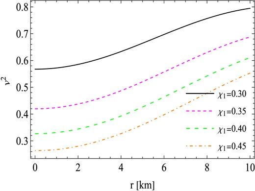
The behavior of velocity of sound (v2) against the radial coordinates r for the values of free parameters γ = −0.0037 km−2, R = 10 km, and χ2 = −0.0024 km−2.

Fig. 5.

The behavior of velocity of sound (v²) against the radial coordinates r for the values of free parameters γ = −0.0037 km⁻², R = 10 km, and χ₂ = −0.0024 km⁻².

Open in new tab Download slide

4.1. Energy conditions

In the context of GR, the concept of energy conditions was well established in the Raychaudhuri equation. This concept can be used in the modified gravity theories as well. In this regard, the energy conditions for a physically realistic model in the |$f(\mathcal {T})$| theory of gravity may be expressed as,

for the weak energy condition (WEC): ρ + E² ≥ 0 and ρ + p ≥ 0;
for the null energy condition (NEC): ρ + p ≥ 0;
for the strong energy condition (SEC): ρ + p ≥ 0, and ρ + 3p − 2E² ≥ 0;
for the dominant energy condition (DEC): ρ − p + 2E² ≥ 0.

In this discussion, we examine the graphical representation of several energy situations, including the WEC, NEC, SEC, and DEC. As it is noted from Figs. 1–3 that the physical parameters q(r), ρ(r), and P(r) are positive throughout the star configuration, therefore, the quantities ρ + E² and ρ + P remain positive everywhere within the star. In order to verify all the energy conditions, it is enough to show the behaviors of the quantities ρ + 3P − 2E² and ρ − P + 2E². The diagrams in Fig. 6 show the behavior of said quantities under the specified constant values of χ₂ = −0.0024 km⁻² and a range of 0.30–0.45 for χ₁, which reveals the fulfillment of energy conditions.

Fig. 6.

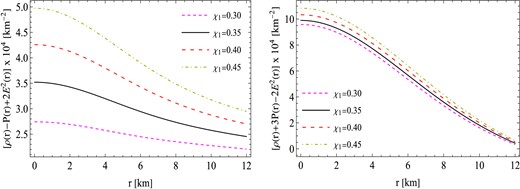
The behavior of energy conditions against the radial coordinates r for similar values of constants to those used in Fig. 5.

Open in new tab Download slide

5. Stability of charged fluid model

5.1. Adiabatic index

Chandrasekhar and Tooper [103] conducted a study to determine the stability or instability of the stellar structure in relation to adiabatic processes. The typical adiabatic index Γ for a consistent Newtonian star is shown to exceed 4/3. Γ does not only define the instability of compact objects, but it also significantly affects the formation, dynamic structure, and oscillation frequencies of the accretion disks that form around these objects [104]. The adiabatic index Γ is larger than 1 if the ratio of pressure to energy density decreases consistently with distance from the center, as shown numerically by Knutsen [105]. It may be inferred that the temperature decreases as one moves out from the center. In this particular instance, the adiabatic coefficient may be calculated as

$$\begin{eqnarray} \Gamma = \frac{\rho +P}{P}\left(\frac{dP}{d\rho }\right). \end{eqnarray}$$

(48)

The variation of the adiabatic index Γ is shown in Fig. 7 for various values of χ₁ while keeping fixed the value of the constant χ₂. The Γ often exhibits a minimal value at the center and increases as one moves outside. The value of Γ at the core with constant χ₂ = −0.0024 km⁻² is as follows: (i) Γ₀ = 2.04614 for χ₁ = 0.30, (ii) Γ₀ = 1.76643 for χ₁ = 0.35, (iii) Γ₀ = 1.57084 for χ₁ = 0.40, and (iv) Γ₀ = 1.42189 for χ₁ = 0.45 (See Table 1). The values of Γ indicate that it exceeds 4/3, demonstrating the attainment of a stable perfect fluid-charged model.

Fig. 7.

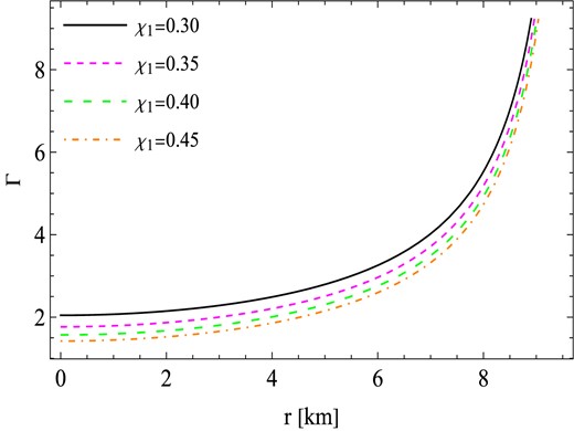
Behavior of the adibatic index (Γ) against the radial coordinates r for similar values of constants to those used in Fig. 5.

Open in new tab Download slide

Table 1.

Open in new tab

The numerical values of the pressure P(r), density ρ(r), constants A and B, central value of the adiabatic index Γ₀, and electric charge (Q).

Parameters	P₀ (dyne/cm²)	ρ₀ (gm/cm³)	ρ_s (gm/cm³)	A	B	Γ₀	\|${Q}\, (C)$\|
χ₁ = 0.30, χ₂ = −0.0024	2.0763 × 10³⁵	6.00903 × 10¹⁴	2.63484 × 10¹⁴	0.0045114	−0.0485865	2.04614	2.35199 × 10²⁰
χ₁ = 0.35, χ₂ = −0.0024	1.93615 × 10³⁵	6.90314 × 10¹⁴	2.96658 × 10¹⁴	0.00422568	−0.0148979	1.76643	2.54044 × 10²⁰
χ₁ = 0.40, χ₂ = −0.0024	1.84413 × 10³⁵	7.79724 × 10¹⁴	3.29833 × 10¹⁴	0.0040114	0.0107053	1.57084	2.71584 × 10²⁰
χ₁ = 0.45, χ₂ = −0.0024	1.78021 × 10³⁵	8.69135 × 10¹⁴	3.63007 × 10¹⁴	0.00384473	0.0308575	1.42189	2.88058 × 10²⁰

Parameters	P₀ (dyne/cm²)	ρ₀ (gm/cm³)	ρ_s (gm/cm³)	A	B	Γ₀	\|${Q}\, (C)$\|
χ₁ = 0.30, χ₂ = −0.0024	2.0763 × 10³⁵	6.00903 × 10¹⁴	2.63484 × 10¹⁴	0.0045114	−0.0485865	2.04614	2.35199 × 10²⁰
χ₁ = 0.35, χ₂ = −0.0024	1.93615 × 10³⁵	6.90314 × 10¹⁴	2.96658 × 10¹⁴	0.00422568	−0.0148979	1.76643	2.54044 × 10²⁰
χ₁ = 0.40, χ₂ = −0.0024	1.84413 × 10³⁵	7.79724 × 10¹⁴	3.29833 × 10¹⁴	0.0040114	0.0107053	1.57084	2.71584 × 10²⁰
χ₁ = 0.45, χ₂ = −0.0024	1.78021 × 10³⁵	8.69135 × 10¹⁴	3.63007 × 10¹⁴	0.00384473	0.0308575	1.42189	2.88058 × 10²⁰

Table 1.

Open in new tab

The numerical values of the pressure P(r), density ρ(r), constants A and B, central value of the adiabatic index Γ₀, and electric charge (Q).

Parameters	P₀ (dyne/cm²)	ρ₀ (gm/cm³)	ρ_s (gm/cm³)	A	B	Γ₀	\|${Q}\, (C)$\|
χ₁ = 0.30, χ₂ = −0.0024	2.0763 × 10³⁵	6.00903 × 10¹⁴	2.63484 × 10¹⁴	0.0045114	−0.0485865	2.04614	2.35199 × 10²⁰
χ₁ = 0.35, χ₂ = −0.0024	1.93615 × 10³⁵	6.90314 × 10¹⁴	2.96658 × 10¹⁴	0.00422568	−0.0148979	1.76643	2.54044 × 10²⁰
χ₁ = 0.40, χ₂ = −0.0024	1.84413 × 10³⁵	7.79724 × 10¹⁴	3.29833 × 10¹⁴	0.0040114	0.0107053	1.57084	2.71584 × 10²⁰
χ₁ = 0.45, χ₂ = −0.0024	1.78021 × 10³⁵	8.69135 × 10¹⁴	3.63007 × 10¹⁴	0.00384473	0.0308575	1.42189	2.88058 × 10²⁰

Parameters	P₀ (dyne/cm²)	ρ₀ (gm/cm³)	ρ_s (gm/cm³)	A	B	Γ₀	\|${Q}\, (C)$\|
χ₁ = 0.30, χ₂ = −0.0024	2.0763 × 10³⁵	6.00903 × 10¹⁴	2.63484 × 10¹⁴	0.0045114	−0.0485865	2.04614	2.35199 × 10²⁰
χ₁ = 0.35, χ₂ = −0.0024	1.93615 × 10³⁵	6.90314 × 10¹⁴	2.96658 × 10¹⁴	0.00422568	−0.0148979	1.76643	2.54044 × 10²⁰
χ₁ = 0.40, χ₂ = −0.0024	1.84413 × 10³⁵	7.79724 × 10¹⁴	3.29833 × 10¹⁴	0.0040114	0.0107053	1.57084	2.71584 × 10²⁰
χ₁ = 0.45, χ₂ = −0.0024	1.78021 × 10³⁵	8.69135 × 10¹⁴	3.63007 × 10¹⁴	0.00384473	0.0308575	1.42189	2.88058 × 10²⁰

5.2. Stability analysis of charged models via Harrison–Zeldovich–Novikov criterion

We apply our findings to meet the Harrison–Zeldovich–Novikov (HZN) stability criterion, as shown in Fig. 8. The following limitations determine whether the HZN stability criterion holds true [106,107]:

$$\begin{eqnarray} \frac{dM}{d\rho _0} &\gt & 0 \rightarrow \mbox{stable configuration}, \end{eqnarray}$$

(49)

$$\begin{eqnarray} \frac{dM}{d\rho _0} &\lt & 0 \rightarrow \mbox{unstable configuration} . \end{eqnarray}$$

(50)

To validate this criterion for the charged solution, we calculate the mass expression as a function of ρ₀ and its derivative with respect to ρ₀ as:

$$\begin{eqnarray} 8\pi \rho _0 = -9 \chi _1 \gamma -\frac{\chi _2}{2}, \end{eqnarray}$$

(51)

$$\begin{eqnarray} M(\rho _0) &=& \frac{1}{24 \chi _1 \Big (R^2 \left(16 \pi \rho _0+\chi _2\right)+9 \chi _1\Big )^2}\Big [18 R^5 \chi _1 \big(32 \pi \rho _0^2-\chi _2^2\big)-2 R^7 \chi _2 \left(16 \pi \rho _0+\chi _2\right)^2 \\ &&+\,\,9 \chi _1^2 \Big (32\pi \rho _0 R^5 \chi _2+32 \pi \rho _0 R^3 \left(8 \pi \rho _0 R^2+9\right)+R^5 \chi _2^2\Big )\Big ], \end{eqnarray}$$

(52)

$$\begin{eqnarray} \frac{d M(\rho _0)}{d\rho _0} &=& \frac{1}{2 \left(R^2 \left(16 \pi +\chi _2\right)+9 \chi _1\right){}^3}\\ &&\times \Big [27 \chi _1 \Big (R^5 (16 \pi \rho _0+\chi _2) +R^3 \chi _1 \left(16 \pi \rho _0 R^2+R^2 \chi _2+9\right)\Big )\Big ]. \end{eqnarray}$$

(53)

From Fig. 8, it is evident that the derivative of M with respect to ρ₀ is positive, implying that the obtained charged models are stable. The upper panel demonstrates that a reduction in the torsion parameter χ₁ results in enhanced stability of the confined structures, but the corresponding increase in mass with respect to the effective central density is minor.

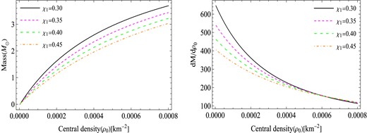
Stability analysis via (left) M–ρ0 and (right) dM/dρ0–ρ0 curves for similar values of constants to those used in Fig. 5.

Fig. 8.

Stability analysis via (left) M–ρ₀ and (right) dM/dρ₀–ρ₀ curves for similar values of constants to those used in Fig. 5.

Open in new tab Download slide

5.3. Hydrostatic equilibrium

To achieve hydrostatic equilibrium, one must analyze the gravitational along with additional fluid forces acting on a dense star, confirming the model’s physical validity. To get a deeper understanding of the equilibrium condition of a charged fluid system in |$f(\mathcal {T})$| gravity, we may examine the generalized Tolman–Oppenheimer–Volkoff (TOV) equation [108,109]:

$$\begin{eqnarray} -\frac{M_G(r)(\rho +P)}{r^2}e^{\frac{\tau -\varphi }{2}}-\frac{dP}{dr}+\frac{q}{4\pi r^4}\frac{dq}{dr}=0, \end{eqnarray}$$

(54)

where M_G(r) is the definition of the effective gravitational mass,

$$\begin{eqnarray} M_G(r)=\frac{1}{2}{{r}^{2}}e^{\frac{\varphi -\tau }{2}}\varphi ^{\prime }. \end{eqnarray}$$

(55)

Then it is easy to derive Eq. (54) as

$$\begin{eqnarray} -\frac{\varphi ^{\prime }}{2}(\rho +P)-\frac{dP}{dr}+\frac{2q}{r^4}\frac{dq}{dr}=0. \end{eqnarray}$$

(56)

The TOV expression (56) characterizes the condition of balance for charged perfect fluid objects subjected to gravitational, hydrostatic, and electric forces. By using the aforementioned formulas, we can formulate the subsequent equation,

$$\begin{eqnarray} F_g+F_h+F_e=0. \end{eqnarray}$$

(57)

The expressions for the forces are as follows: |$F_g=-\frac{\varphi ^{\prime }}{2}(\rho +P)$|⁠, |$F_h=-\frac{dp}{dr}$|⁠, and |$F_e=\frac{2q}{r^4} \frac{dq}{dr}$|⁠. Subsequently, we plot Fig. 9 to depict the objective of fulfilling the aforementioned equation that asserts the total of these three forces is 0. The model claims that the gravitational force (F_g) is canceled out by the combined influence of the hydrostatic force (F_h) and electric force (F_e) to maintain a state of equilibrium.

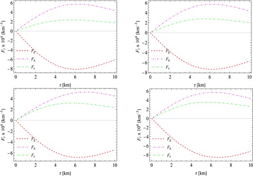
The behavior of different forces against the radial coordinates r for the values of free parameters γ = −0.0037 km−2, R = 10 km, and χ2 = −0.0024 km−2 with different values of α. (Top left) χ1 = 0.30, (top right) χ1 = 0.35, (bottom left) χ1 = 0.40, (bottom right) χ1 = 0.45.

Fig. 9.

The behavior of different forces against the radial coordinates r for the values of free parameters γ = −0.0037 km⁻², R = 10 km, and χ₂ = −0.0024 km⁻² with different values of α. (Top left) χ₁ = 0.30, (top right) χ₁ = 0.35, (bottom left) χ₁ = 0.40, (bottom right) χ₁ = 0.45.

Open in new tab Download slide

6. Influence of the torsion parameter χ₁ and electric charge Q on mass–radius relation for different compact objects via M–R curves

The upper and lower bounds on the mass–radius ratio in the presence of a cosmological constant were derived by Andréasson [110] and Böhmer and Harko [111], respectively. In the context of |$f(\mathcal {T})$| gravity, the inequality expressing the bounds on the mass–radius ratio can be formulated as follows:

$$\begin{eqnarray} \left (\frac{3 {Q}^2}{4R^2}+\frac{\chi _{_2} R^2}{24 \chi _{_1}} \right ) \le \frac{{M}}{R} \le \left ( \frac{2}{9}+\frac{{Q}^2}{3R^2}-\frac{\chi _{_2} R^2}{18\chi _{_1}}+\frac{2}{9} \sqrt{1+\frac{3{Q}^2}{R^2}+\frac{3\chi _{_2} R^2}{2 \chi _{_1}}} \right ). \end{eqnarray}$$

(58)

Let us now shift our focus to investigating the characteristics of compact astronomical objects through the analysis of M–R curves produced by our phenomenal system. Specifically, we will explore pulsars, which belong to a class of celestial objects known as NSs. Pulsars are distinguished by their remarkably strong magnetic fields and their ability to emit periodic bursts of electromagnetic signals, commonly referred to as pulses. The origin of these pulses is attributed to the combination of their intense magnetic fields and rapid rotation. The high rotational frequencies observed in pulsars suggest that they must be exceptionally compact. Typically, pulsars are found within binary systems, where a massive NS is accompanied by another star. These binary systems, governed by Kepler’s third law, offer a unique opportunity to measure the mass of the NS. By analyzing the time delays in the arrival of pulses, scientists can extract valuable information about the mass of the NS. This measurement technique has been studied extensively, as referenced by Lattimer [112] and Ozel et al. [113].

In our investigation of the M–R relationship within the framework of f(Q) gravity, we have focused on studying the effect of the torsion parameter χ₁ and electric charge Q on various compact objects. Specifically, we have selected the following objects for our analysis: Her X-1, LMC X-4, PSR J1903+327, PSR J1614-2230, and GW190814. The existence of these compact objects is inherently supported by a stiff EoS, which allows for relatively higher pressure values while maintaining fixed energy density. In this context, the pressure within the NS configuration plays a significant role in counteracting the gravitational collapse of matter. The determination of NS radii is a complex task that can be facilitated by advancements in theoretical modeling. In this study, we have developed a framework for constructing models of compact objects within the context of f(Q) gravity. Significantly, in Fig. 10 (left panel), we have depicted the relationship between the total mass M (normalized in solar masses, M_⊙) and the radius R for the considered compact object candidates, using selected values of χ₁ (0.30, 0.35, 0.40, 0.45, and 0.50). The figure illustrates that the maximum mass (M_max) gradually increases as the value of χ₁ ranges from 0.30 to 0.50. In Table 2, we present the maximum allowable masses and their corresponding radii for different values of χ₁ within our model. Specifically, the maximum masses in our model range from 0.70M_⊙ to 2.67M_⊙, while the corresponding radii span from 8.47 km to 11.33 km. Our analysis demonstrates that the masses of the mentioned five compact objects can be achieved within our proposed mode, by selecting different values of χ₁. In Fig. 11 (left panel), we present the correlation between the total mass M (normalized in solar masses, M_⊙) and the radius R for the same set of compact object candidates. However, in this case, we vary the values of Q (0.0, 0.5, 1, 1.5, and 2). The plot illustrates that the maximum mass (M_max) gradually decreases as the value of Q increases from 0 to 2. In Table 3, we provide details on the maximum allowable masses and their corresponding radii for different values of Q within our model. Specifically, the maximum masses in our model range from 0.70M_⊙ to 2.67M_⊙, while the corresponding radii range from 13.85 km to 15.36 km. Our analysis demonstrates that the masses of the mentioned five compact objects can also be successfully accounted for within our proposed model by selecting different values of Q. Clearly, M–R curves exhibiting larger values of χ₁ and smaller values of χ₁ correspond to a stiffer EoS. This observation is indicative of the presence of massive NSs within the system.

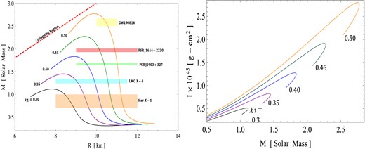
Influence of the torsion parameter χ1 on (left) mass–radius and (right) M–I relations for different compact objects via the M–R curve.

Fig. 10.

Influence of the torsion parameter χ₁ on (left) mass–radius and (right) M–I relations for different compact objects via the M–R curve.

Open in new tab Download slide

Fig. 11.

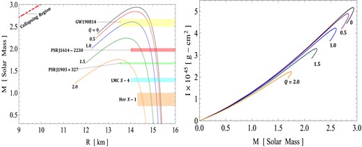
Influence of the electric charge Q on (left) mass–radius and (right) M–I relations for different compact objects via the M–R curve.

Open in new tab Download slide

Table 2.

Open in new tab

M–R curve and prediction of radii for different values of χ₁.

Objects	M/M_⊙	Predicted R [km]
		χ₁ = 0.30	χ₁ = 0.35	χ₁ = 0.40	χ₁ = 0.45	χ₁ = 0.50
Her X-1	0.85 ± 0.15	\|$8.69^{+0.20}_{-0.22}$\|	\|$9.49^{+0.14}_{-0.15}$\|	\|$10.15^{+0.10}_{-0.08}$\|	\|$10.73^{+0.09}_{-0.07}$\|	\|$11.25^{+0.08}_{-0.05}$\|
LMC X-4	1.29 ± 0.05	–	\|$9.02^{+0.08}_{-0.09}$\|	\|$9.89^{+0.04}_{-0.03}$\|	\|$10.55^{+0.03}_{-0.01}$\|	\|$11.12^{+0.01}_{-0.01}$\|
PSR J1903+327	1.667 ± 0.021	–	–	\|$9.52^{+0.03}_{-0.02}$\|	\|$10.37^{+0.02}_{-0.01}$\|	\|$11.01^{+0.01}_{-0.01}$\|
PSR J1614-2230	1.97 ± 0.04	–	–	–	\|$10.15^{+0.04}_{-0.04}$\|	\|$10.90^{+0.02}_{-0.01}$\|
GW190814	2.5–2.67	–	–	–	–	\|$10.49^{+0.07}_{-0.16}$\|

Objects	M/M_⊙	Predicted R [km]
		χ₁ = 0.30	χ₁ = 0.35	χ₁ = 0.40	χ₁ = 0.45	χ₁ = 0.50
Her X-1	0.85 ± 0.15	\|$8.69^{+0.20}_{-0.22}$\|	\|$9.49^{+0.14}_{-0.15}$\|	\|$10.15^{+0.10}_{-0.08}$\|	\|$10.73^{+0.09}_{-0.07}$\|	\|$11.25^{+0.08}_{-0.05}$\|
LMC X-4	1.29 ± 0.05	–	\|$9.02^{+0.08}_{-0.09}$\|	\|$9.89^{+0.04}_{-0.03}$\|	\|$10.55^{+0.03}_{-0.01}$\|	\|$11.12^{+0.01}_{-0.01}$\|
PSR J1903+327	1.667 ± 0.021	–	–	\|$9.52^{+0.03}_{-0.02}$\|	\|$10.37^{+0.02}_{-0.01}$\|	\|$11.01^{+0.01}_{-0.01}$\|
PSR J1614-2230	1.97 ± 0.04	–	–	–	\|$10.15^{+0.04}_{-0.04}$\|	\|$10.90^{+0.02}_{-0.01}$\|
GW190814	2.5–2.67	–	–	–	–	\|$10.49^{+0.07}_{-0.16}$\|

Table 2.

Open in new tab

M–R curve and prediction of radii for different values of χ₁.

Objects	M/M_⊙	Predicted R [km]
		χ₁ = 0.30	χ₁ = 0.35	χ₁ = 0.40	χ₁ = 0.45	χ₁ = 0.50
Her X-1	0.85 ± 0.15	\|$8.69^{+0.20}_{-0.22}$\|	\|$9.49^{+0.14}_{-0.15}$\|	\|$10.15^{+0.10}_{-0.08}$\|	\|$10.73^{+0.09}_{-0.07}$\|	\|$11.25^{+0.08}_{-0.05}$\|
LMC X-4	1.29 ± 0.05	–	\|$9.02^{+0.08}_{-0.09}$\|	\|$9.89^{+0.04}_{-0.03}$\|	\|$10.55^{+0.03}_{-0.01}$\|	\|$11.12^{+0.01}_{-0.01}$\|
PSR J1903+327	1.667 ± 0.021	–	–	\|$9.52^{+0.03}_{-0.02}$\|	\|$10.37^{+0.02}_{-0.01}$\|	\|$11.01^{+0.01}_{-0.01}$\|
PSR J1614-2230	1.97 ± 0.04	–	–	–	\|$10.15^{+0.04}_{-0.04}$\|	\|$10.90^{+0.02}_{-0.01}$\|
GW190814	2.5–2.67	–	–	–	–	\|$10.49^{+0.07}_{-0.16}$\|

Objects	M/M_⊙	Predicted R [km]
		χ₁ = 0.30	χ₁ = 0.35	χ₁ = 0.40	χ₁ = 0.45	χ₁ = 0.50
Her X-1	0.85 ± 0.15	\|$8.69^{+0.20}_{-0.22}$\|	\|$9.49^{+0.14}_{-0.15}$\|	\|$10.15^{+0.10}_{-0.08}$\|	\|$10.73^{+0.09}_{-0.07}$\|	\|$11.25^{+0.08}_{-0.05}$\|
LMC X-4	1.29 ± 0.05	–	\|$9.02^{+0.08}_{-0.09}$\|	\|$9.89^{+0.04}_{-0.03}$\|	\|$10.55^{+0.03}_{-0.01}$\|	\|$11.12^{+0.01}_{-0.01}$\|
PSR J1903+327	1.667 ± 0.021	–	–	\|$9.52^{+0.03}_{-0.02}$\|	\|$10.37^{+0.02}_{-0.01}$\|	\|$11.01^{+0.01}_{-0.01}$\|
PSR J1614-2230	1.97 ± 0.04	–	–	–	\|$10.15^{+0.04}_{-0.04}$\|	\|$10.90^{+0.02}_{-0.01}$\|
GW190814	2.5–2.67	–	–	–	–	\|$10.49^{+0.07}_{-0.16}$\|

Table 3.

Open in new tab

M–R curve and prediction of radii for different values of Q.

Objects	M/M_⊙	Predicted R [km]
		Q = 0.0	Q = 0.5	Q = 1.0	Q = 1.5	Q = 2.0
Her X-1	0.85 ± 0.15	\|$15.34^{+0.02}_{-0.02}$\|	\|$15.29^{+0.02}_{-0.02}$\|	\|$15.16^{+0.02}_{-0.02}$\|	\|$14.91^{+0.04}_{-0.03}$\|	\|$14.52^{+0.06}_{-0.05}$\|
LMC X-4	1.29 ± 0.05	\|$15.28^{+0.01}_{-0.01}$\|	\|$15.24^{+0.01}_{-0.01}$\|	\|$15.08^{+0.01}_{-0.01}$\|	\|$14.81^{+0.01}_{-0.02}$\|	\|$14.32^{+0.03}_{-0.04}$\|
PSR J1903+327	1.667 ± 0.021	\|$15.21^{+0.01}_{-0.01}$\|	\|$15.17^{+0.01}_{-0.01}$\|	\|$14.99^{+0.01}_{-0.01}$\|	\|$14.66^{+0.01}_{-0.01}$\|	\|$13.89^{+0.06}_{-0.04}$\|
PSR J1614-2230	1.97 ± 0.04	\|$15.15^{+0.01}_{-0.01}$\|	\|$15.08^{+0.01}_{-0.02}$\|	\|$14.89^{+0.02}_{-0.02}$\|	\|$14.46^{+0.03}_{-0.04}$\|	–
GW190814	2.5–2.67	\|$14.91^{+0.04}_{-0.07}$\|	\|$14.80^{+0.05}_{-0.09}$\|	\|$14.32^{+0.16}_{-}$\|	–	–

Objects	M/M_⊙	Predicted R [km]
		Q = 0.0	Q = 0.5	Q = 1.0	Q = 1.5	Q = 2.0
Her X-1	0.85 ± 0.15	\|$15.34^{+0.02}_{-0.02}$\|	\|$15.29^{+0.02}_{-0.02}$\|	\|$15.16^{+0.02}_{-0.02}$\|	\|$14.91^{+0.04}_{-0.03}$\|	\|$14.52^{+0.06}_{-0.05}$\|
LMC X-4	1.29 ± 0.05	\|$15.28^{+0.01}_{-0.01}$\|	\|$15.24^{+0.01}_{-0.01}$\|	\|$15.08^{+0.01}_{-0.01}$\|	\|$14.81^{+0.01}_{-0.02}$\|	\|$14.32^{+0.03}_{-0.04}$\|
PSR J1903+327	1.667 ± 0.021	\|$15.21^{+0.01}_{-0.01}$\|	\|$15.17^{+0.01}_{-0.01}$\|	\|$14.99^{+0.01}_{-0.01}$\|	\|$14.66^{+0.01}_{-0.01}$\|	\|$13.89^{+0.06}_{-0.04}$\|
PSR J1614-2230	1.97 ± 0.04	\|$15.15^{+0.01}_{-0.01}$\|	\|$15.08^{+0.01}_{-0.02}$\|	\|$14.89^{+0.02}_{-0.02}$\|	\|$14.46^{+0.03}_{-0.04}$\|	–
GW190814	2.5–2.67	\|$14.91^{+0.04}_{-0.07}$\|	\|$14.80^{+0.05}_{-0.09}$\|	\|$14.32^{+0.16}_{-}$\|	–	–

Table 3.

Open in new tab

M–R curve and prediction of radii for different values of Q.

Objects	M/M_⊙	Predicted R [km]
		Q = 0.0	Q = 0.5	Q = 1.0	Q = 1.5	Q = 2.0
Her X-1	0.85 ± 0.15	\|$15.34^{+0.02}_{-0.02}$\|	\|$15.29^{+0.02}_{-0.02}$\|	\|$15.16^{+0.02}_{-0.02}$\|	\|$14.91^{+0.04}_{-0.03}$\|	\|$14.52^{+0.06}_{-0.05}$\|
LMC X-4	1.29 ± 0.05	\|$15.28^{+0.01}_{-0.01}$\|	\|$15.24^{+0.01}_{-0.01}$\|	\|$15.08^{+0.01}_{-0.01}$\|	\|$14.81^{+0.01}_{-0.02}$\|	\|$14.32^{+0.03}_{-0.04}$\|
PSR J1903+327	1.667 ± 0.021	\|$15.21^{+0.01}_{-0.01}$\|	\|$15.17^{+0.01}_{-0.01}$\|	\|$14.99^{+0.01}_{-0.01}$\|	\|$14.66^{+0.01}_{-0.01}$\|	\|$13.89^{+0.06}_{-0.04}$\|
PSR J1614-2230	1.97 ± 0.04	\|$15.15^{+0.01}_{-0.01}$\|	\|$15.08^{+0.01}_{-0.02}$\|	\|$14.89^{+0.02}_{-0.02}$\|	\|$14.46^{+0.03}_{-0.04}$\|	–
GW190814	2.5–2.67	\|$14.91^{+0.04}_{-0.07}$\|	\|$14.80^{+0.05}_{-0.09}$\|	\|$14.32^{+0.16}_{-}$\|	–	–

Objects	M/M_⊙	Predicted R [km]
		Q = 0.0	Q = 0.5	Q = 1.0	Q = 1.5	Q = 2.0
Her X-1	0.85 ± 0.15	\|$15.34^{+0.02}_{-0.02}$\|	\|$15.29^{+0.02}_{-0.02}$\|	\|$15.16^{+0.02}_{-0.02}$\|	\|$14.91^{+0.04}_{-0.03}$\|	\|$14.52^{+0.06}_{-0.05}$\|
LMC X-4	1.29 ± 0.05	\|$15.28^{+0.01}_{-0.01}$\|	\|$15.24^{+0.01}_{-0.01}$\|	\|$15.08^{+0.01}_{-0.01}$\|	\|$14.81^{+0.01}_{-0.02}$\|	\|$14.32^{+0.03}_{-0.04}$\|
PSR J1903+327	1.667 ± 0.021	\|$15.21^{+0.01}_{-0.01}$\|	\|$15.17^{+0.01}_{-0.01}$\|	\|$14.99^{+0.01}_{-0.01}$\|	\|$14.66^{+0.01}_{-0.01}$\|	\|$13.89^{+0.06}_{-0.04}$\|
PSR J1614-2230	1.97 ± 0.04	\|$15.15^{+0.01}_{-0.01}$\|	\|$15.08^{+0.01}_{-0.02}$\|	\|$14.89^{+0.02}_{-0.02}$\|	\|$14.46^{+0.03}_{-0.04}$\|	–
GW190814	2.5–2.67	\|$14.91^{+0.04}_{-0.07}$\|	\|$14.80^{+0.05}_{-0.09}$\|	\|$14.32^{+0.16}_{-}$\|	–	–

In the context of f(Q) gravity, it is worth mentioning that the secondary mass of GW190814 falls within the hypothesized lower “mass gap” range of (2.5–5) M_⊙, which is believed to exist between known NSs and BHs [113–116]. This secondary mass is heavier than the most massive pulsar in the galaxy [117] and nearly surpasses the mass of the primary component of GW190425, which falls within the range of (1.61–2.52) M_⊙ and is considered an outlier compared to the population of binary NS systems in our galaxy [118]. Furthermore, it is comparable to the mass of the millisecond pulsar PSR J1748-2021B [119], which has a claimed mass of |$2.74_{-0.21}^{+0.21}~M_{\odot }$| at a 68% confidence level.

A significant discovery in this study within the context of f(Q) gravity is the identification of a compact object with a mass of 2.57 M_⊙ that falls within the proposed lower range of the “mass gap,” specifically for χ₁ = 0.5 and Q ≤ 1. Remarkably, our findings align with the new data for PSR J0952-0607, which exhibits a mass of |$2.35_{-0.17}^{+0.17}~M_{\odot }$|⁠. PSR J0952-0607 stands as the most massive and fastest pulsar within the Milky Way’s disk, and its characteristics lend support to the potential existence of strange quark matter within its composition. This binary millisecond pulsar, operating at a frequency of 707 Hz, was initially reported by Bassa et al. [120] and is commonly referred to as a “black widow binary” due to the pulsar’s intense luminosity causing irradiation and evaporation of its low-mass (substellar) companion.

In a different study by Astashenok et al. [16], the R² model scenario was examined, revealing that it adheres to the general relativistic limit of approximately 3M_⊙. The upper causal mass limit was found to marginally match the general relativistic causal maximum mass and fall within the mass gap region. The authors also explored the concept of strange stars within the context of modified gravity, specifically in relation to the secondary component of the GW190814 event. Furthermore, Odintsov and Oikonomou [121] investigated static NSs using various inflationary models popular in cosmology. By employing the MPA1 EoS, the authors demonstrated that the maximum masses of NSs resided within the mass gap region, with values exceeding 2.5 M_⊙ but remaining below the causal limit of 3 solar masses.

7. Impact of slow rotation and moment of inertia

According to Newtonian theory, relativistic bodies are no longer stationary in connection to astronomical stellar objects [122]. On the other hand, the present gravitational body is influenced by the rotational movement of the fluid. This phenomenon, based on the laws of GR, was first examined by Thirring in 1918 [123], and subsequently explored in more depth by Brill and Cohen in 1966 [124], shedding light on its relationship with Mach’s principle. Precisely determining the rotational speed is crucial for achieving equilibrium between the forces of gravity, pressure, and centrifugal forces. Now, we will analyze the influence of a slow rotation on these configurations. The study of the masses and radii of X-ray radio pulsars is now an emerging discipline in observational astrophysics. Determining the moment of inertia is crucial for accurately simulating these radio pulsars. Recent studies have examined Millisecond X-Ray Pulsar MAXI J1816–195 [125] using the Neutron Star Interior Composition Explorer (NICER) Telescope, millisecond Pulsar PSR J0514-4002E [126] using the Karoo Array Telescope (MeerKAT), whereas X-ray pulsars 1E 1145.1-6141 [127] and IGR J19294+1816 [128] have been examined using data from the Nuclear Spectroscopic Telescope Array mission (NuSTAR). Various methods may be used to figure out the stiffness of an EoS, such as calculating the adiabatic index or the sound speed. Nevertheless, the M–R and I–M plots exhibit a rather acute sensitivity to stiffness. The I–M graph is highly efficient and accurate in measuring the stiffness of an EoS. In order to make a comparison with the I–M curve, it is necessary to know the method for calculating the moment of inertia (I). By using the Bejger and Haensel [129] formula, one may calculate the moment of inertia (I) that corresponds to a static solution. The expression is derived from

$$\begin{eqnarray} I = \frac{2}{9} \Bigg ( 1+\frac{5(M/R).\mathrm{ km} }{M_{\odot }} M R^2\Bigg ). \end{eqnarray}$$

(59)

Accordingly, Baskey et al. [130] quantify the slow rotation impact of pulsars in the context of GR. In this study, we have plotted the moment of inertia against mass in the right panels of Figs. 10 and 11 for different values of the torsion parameter χ₁ and electric charge Q. As the mass increases with the χ₁ parameter, the moment of inertia also increases. The obtained values of maximum mass and moment of inertia for different values of torsion parameter are as follows:

For χ₁ = 0.30: M_max = 1.118M_⊙ and I = 4.90 × 10⁴⁴g · cm²;
For χ₁ = 0.35: M_max = 1.453M_⊙ and I = 8.15 × 10⁴⁴g · cm²;
For χ₁ = 0.40: M_max = 1.83M_⊙ and I = 1.25 × 10⁴⁵g · cm²;
For χ₁ = 0.45: M_max = 2.27M_⊙ and I = 1.89 × 10⁴⁵g · cm²;
For χ₁ = 0.50: M_max = 2.77M_⊙ and I = 2.78 × 10⁴⁵g · cm².

However, as the charge increases the moment of inertia decreases and the corresponding values are:

For Q = 0.0: M_max = 2.94M_⊙ and I = 5.15 × 10⁴⁵g · cm²;
For Q = 0.5: M_max = 2.84M_⊙ and I = 4.88 × 10⁴⁵g · cm²;
For Q = 1.0: M_max = 2.61M_⊙ and I = 4.23 × 10⁴⁵g · cm²;
For Q = 1.5: M_max = 2.24M_⊙ and I = 3.29 × 10⁴⁵g · cm²;
For Q = 2.0: M_max = 1.75M_⊙ and I = 2.23 × 10⁴⁵g · cm².

Comparing the left and right panels of Fig. 10 shows that the mass obtained for the nonrotating star is more than the slow-rotating star for all values of χ₁, whereas the situation is reversed when we vary electric charge Q, see Fig. 11.

8. Concluding remarks

In this paper, we present a new and exact solution for a charged spherical model within the framework of |$f(\mathcal {T})$| gravity. By solving the field equation using a well-behaved ansatz for the radial component of the metric function and an appropriate form of the electric field, we derive this solution. Our main objective is to provide a thorough understanding of charged anisotropic compact stars. Moreover, we extensively examine how the structural physical parameters of the model, as well as the model parameters, vary under specific physical conditions. Particularly, we investigate the influence of the torsion parameter and electric charge on compact stars in lower mass gaps. By conducting this analysis, we deepen our understanding of the distinctive features exhibited by charged anisotropic compact stars within the framework of |$f(\mathcal {T})$| gravity, leading to a more accurate explanation of their behavior.

What’s more, our analysis provides valuable insights into the behavior and characteristics of charged anisotropic compact stars within the arena of |$f(\mathcal {T})$| gravity. We demonstrate the regularity and positivity of the metric coefficients, ensuring the physical viability of the solutions. The presence of a positive electric charge in the compact star leads to a repulsive force that counteracts gravitational collapse and maintains equilibrium. We observe that the electric charge increases from the center to the boundary of the star, indicating an outward electric force throughout the stellar interior. Furthermore, we examine the energy density, pressure, and ratio of pressure to density of the compact star. The energy density is highest at the core and decreases towards the surface. The pressure remains finite throughout the stellar interior, with the highest values at the center and the lowest at the surface. The ratio of pressure to density is consistently lower than unity, providing insights into the nature of the stellar matter. Additionally, we confirm that the speed of sound within the fluid remains below the speed of light, satisfying the causality requirements.

The extent to which different energy conditions and stability criteria are satisfied for the charged anisotropic compact star models is also examined in the context of |$f(\mathcal {T})$| gravity. We find that the physical parameters, such as the charge density q(r), energy density ρ(r), and pressure P(r), are positive throughout the stellar configuration, ensuring that quantities like ρ + E² and ρ + P remain positive as well. By studying the behavior of the quantities ρ + 3P − 2E² and ρ − P + 2E², we confirm that the energy conditions, including the WEC, NEC, SEC, and DEC, are satisfied. However, we have analyzed the adiabatic index Γ, which exhibits a minimum value at the center of the star and increases towards the outer regions. The values of Γ exceed 4/3, indicating the attainment of a stable perfect fluid-charged model. The derivative of the gravitational mass M with respect to the central energy density ρ₀ is found to be positive, indicating stability of the charged models. Furthermore, we demonstrate the fulfillment of the TOV equation, which states that the total of the gravitational force, hydrostatic force, and electric force must sum to 0 in order to maintain equilibrium. We have shown that the three forces balance each other, ensuring a stable equilibrium state.

Our investigation into the relationship between the mass and radius (M–R) of compact astronomical objects, particularly pulsars and other similar objects, has yielded intriguing results. By varying the torsion parameter χ₁ and electric charge Q, we observe significant effects on the maximum mass (M_max) and the corresponding radii of these objects. Increasing values of χ₁ lead to higher M_max and smaller radii, indicating the possibility of the existence of massive NSs within the system. On the other hand, increasing values of Q result in a decrease in M_max and larger radii. Furthermore, our analysis reveals that the masses of the compact object candidates can be accurately accommodated within our proposed model by choosing different values for χ₁ and Q. The M–R curves exhibit a correlation between larger values of χ₁ and smaller values of Q with a stiffer EoS, suggesting the presence of massive compact objects. These findings contribute to our understanding of the properties and composition of compact astronomical objects, shedding light on the behavior of matter under extreme conditions and the nature of gravity. Our study has uncovered significant implications, particularly regarding the secondary mass of GW190814. This secondary mass falls within the hypothesized lower “mass gap” range of (2.5–5) M_⊙, which offers support for the existence of a distinct mass gap between known NSs and BHs. This mass is notably greater than the most massive pulsar in the galaxy and nearly surpasses the mass of the primary component of GW190425, which is considered an outlier compared to the population of binary NS systems in our galaxy. Additionally, the secondary mass is comparable to the mass of the millisecond pulsar PSR J1748-2021B, further highlighting the significance of our findings. Moreover, we have obtained a compact object with a mass of 2.57 M_⊙ that falls within the hypothesized lower “mass gap” range. This result aligns with the new data for PSR J0952-0607, which is the heaviest and fastest pulsar in the Milky Way’s disk. The properties of PSR J0952-0607 also lend support to the possibility of strange quark matter existing in its composition. This pulsar, known as a “black widow binary,” features a 707 Hz binary millisecond pulsar and has been previously reported by Bassa et al. [120]. It is worth noting that Astashenok and Odintsov [131] have conducted a study on realistic NSs within the framework of axion R² gravity. The authors make a significant discovery regarding the potential existence of supermassive compact stars with masses around M ≈ 2.2–2.3 M_⊙ and radii approximately R_s ≈ 11 km. These predictions are based on a realistic EoS, specifically considering the APR EoS. Additionally, the study reveals an intriguing result related to the behavior of the scalar curvature in comparison to vacuum R² gravity. The authors find that the scalar curvature decays at a slower rate due to the presence of an axion “galo” around the star. On the other hand, the work by Nashed et al. [132] delves into the study of spherically symmetric spacetime solutions for the interior of stellar compact objects in the higher-order curvature theory. Their findings reveal the ability of their model to bypass the necessary conditions for compact anisotropic stars, with a specific focus on the Her X-1 star. Additionally, the authors highlight the differentiated and enhanced stability of their proposed model compared to analogous models within the framework of GR. In a more recent study, Astashenok et al. [133] delve into realistic models of compact objects, focusing on NSs and SSs, which incorporate dense matter and dark energy. The study explores various scenarios, including a simple fluid or scalar field interacting with matter as the dark energy component. Additionally, the authors investigate the effects of modified gravity by examining the R² model in combination with dark energy. Finally, the study considers the case of dark energy as a scalar field nonminimally interacting with gravity, offering a comprehensive analysis of the interconnections between these components.

We have also explored the relationship between the moment of inertia and mass for various values of the torsion parameter χ₁ and electric charge Q. Our findings demonstrate that increasing the mass with respect to χ₁ leads to a corresponding increase in the moment of inertia. We have determined the maximum mass and the accompanying moment of inertia for different χ₁ values. Conversely, as the electric charge is increased, the moment of inertia exhibits a decrease. An intriguing observation arises from comparing the results: for all χ₁ values, nonrotating stars possess higher masses compared to slow-rotating stars, whereas this trend is reversed when adjusting the electric charge Q.

In conclusion, the results of this experiment have unambiguously shown the material importance and practicality of incorporating the torsion parameter and electric charge into the study of compact stars in the lower mass range, particularly in the context of |$f(\mathcal {T})$| gravity. These influential factors have been shown to have a profound impact on the characteristics and dynamics of compact stars, underlining their crucial role in advancing our understanding of the underlying physics governing these astrophysical objects.

Acknowledgement

The authors are thankful to the Deanship of Graduate Studies and Scientific Research at University of Bisha for supporting this work through the Fast-Track Research Support Program. A.E. thanks the National Research Foundation of South Africa for the award of a postdoctoral fellowship. S.K.M. thanks the administration of University of Nizwa for their ongoing assistance and encouragement in doing this research study. G.M. is very thankful to Prof. Gao Xianlong from the Department of Physics, Zhejiang Normal University, for his kind support and help during this research. Further, G.M. acknowledges grant no. ZC304022919 to support his Postdoctoral Fellowship at Zhejiang Normal University, People’s Republic of China.

Funding

Data availability

This paper does not have any supporting data or the data will not be archived. The required numerical results and graphical analysis are already included in the manuscript.

References

[1]

H. F. M.

Goenner

Living Rev. Rel.

(

2004

Month:	Total Views:
March 2024	33
April 2024	138
May 2024	80
June 2024	49
July 2024	48
August 2024	36
September 2024	38
October 2024	18
November 2024	21
December 2024	12
January 2025	28
February 2025	11
March 2025	25
April 2025	10
May 2025	12

Article Contents

Charged Spherical Solution in Torsion and Matter Coupling Gravity and Influence of Torsion Parameter and Electric Charge on Compact Stars in Lower Mass Gap

Abstract

1. Introduction

2. Static spherical symmetry field equation in T gravity

3. Boundary conditions

4. Physical analysis

4.1. Energy conditions

5. Stability of charged fluid model

5.1. Adiabatic index

5.2. Stability analysis of charged models via Harrison–Zeldovich–Novikov criterion

5.3. Hydrostatic equilibrium

6. Influence of the torsion parameter χ1 and electric charge Q on mass–radius relation for different compact objects via M–R curves

7. Impact of slow rotation and moment of inertia

8. Concluding remarks

Acknowledgement

Funding

Data availability

References

Author notes

Citations

Views

Altmetric

Email alerts

Astrophysics Data System

Citing articles via

Latest

Most Read

Most Cited

This Feature Is Available To Subscribers Only

6. Influence of the torsion parameter χ₁ and electric charge Q on mass–radius relation for different compact objects via M–R curves