


Abstract
The excess-path-length distribution of cascade-shower particles due to the multiple Coulomb scattering of shower electrons is investigated analytically. A diffusion equation for the distribution under the Landau approximation is proposed and solved under the conditions of neglecting and including the ionization loss. Contributions of the Rutherford single scattering on the distribution are also investigated and found to dominate in very large excess regions of path length. The excess-path-length distribution of shower electrons is observed as an arrival-time distribution at a given thickness of traverse. The present results will be valuable for qualitative and quantitative analyses of cascade showers observed by the arrival-time distribution.
1. Introduction
High-energy electrons (including positrons, in this report) traversing through matter produce secondary photons by radiation, sharing energies of the primary electron between the secondary photon and the surviving electron. On the other hand, high-energy photons traversing through matter produce electron pairs by pair production, sharing energies of the primary photon between the pair electrons. As a consequence, they produce electromagnetic cascade showers, as reviewed in Rossi and Greisen [1] and Nishimura [2], where the numbers of electrons and photons above some threshold energies increase, reach some peaks, and begin to decrease afterwards, with the increase of traversed thickness in matter configuring the transition curves indicated in Refs. [1,2].
However, at a given thickness of traverse, the shower shows other important characteristics. Shower particles shift their locations sideways from the shower axis as they change their directions of motion from the incident direction of the shower, due to the multiple Coulomb scattering of electrons with the matter of traverse obeying Fermi’s formulae (see Section 23 of Ref. [1]). Therefore they show a lateral distribution of location in the shower as predicted by Kamata and Nishimura [2,3]. At the same time, shower particles shift their locations backward from the shower front or the tangential plane at the traversed thickness as their path lengths exceed the thickness of traverse with their direction angles inclined, due to the above scattering of electrons obeying Yang’s additional formulae [4,5]. Therefore they show the excess-path-length (EPL) distribution or the longitudinal distribution of location in the shower that is observed as an arrival-time distribution of shower electrons [6–10].
We investigate this distribution of shower electrons by first proposing a diffusion equation under the Landau approximation (Fokker–Planck approximation) [2,3] and solving the equation under the conditions of neglecting and including the ionization loss of electrons (Approximations A and B) [1,2,]1, in matter of uniform density. Contributions of Rutherford single scattering on the EPL distribution of shower electrons in very large excess regions are investigated next by applying single scattering to the shower electrons, assuming shower particles to propagate straight toward the directions of shower development before and after the single scattering. The results for both are compared in figures, and contributions of both on the analyses of EPL distribution are discussed.
2. The EPL distribution of cascade-shower electrons under Approximation A
2.1. The diffusion equation under Approximation A
Let |$\pi (E,\vec{\theta },\Delta ,t)dE d\vec{\theta } d\Delta$| and |$\gamma (E,\vec{\theta },\Delta ,t)dE d\vec{\theta } d\Delta$| be the numbers of electrons and photons of energy E, direction |$\vec{\theta }$|, and EPL Δ [4,5] within the infinitesimal ranges of dE, |$d\vec{\theta }$|, and dΔ, at the traversed thickness of t in units of radiation length [1,2]. Under the cascade process described in Kamata and Nishimura [2,3], the density π for the direction angle |$\vec{\theta }$| increases by |$(E_{\rm s}^2/4E^2)\nabla _\theta ^2\pi dt$| due to multiple Coulomb scattering [1,2] under the Landau approximation [2,3] and the densities π and γ at the EPL Δ change by an increase of |$d\Delta = (\sec \theta -1) dt \simeq (\theta ^2/2) dt$| after the infinitesimal traverse of dt. Therefore we have a diffusion equation of
under the Landau approximation with the ionization loss of electrons neglected (Approximation A), where the operators A′, B′, C′ and the constant σ0 are defined in Kamata and Nishimura [2,3] and the densities are expressed as π(E, θ, Δ, t) and γ(E, θ, Δ, t) as they are axially symmetric with |$\vec{\theta }$|.
After applying Mellin, Laplace, and Hankel transforms to the densities π and γ as
the diffusion equation (1) becomes
We express f and g by series expansion of
then Eq. (3) becomes
as they satisfy A′E−s − 1 = A(s)E−s − 1, B′E−s − 1 = B(s)E−s − 1, and C′E−s − 1 = C(s)E−s − 1, where A(s), B(s), and C(s) are the cascade functions defined in Refs. [1,2].
We introduce the inverse matrix of the coefficient matrix on the left-hand side,
where λ1(s) and λ2(s) are defined in Refs. [1,2]. Then, multiplying Rs + 2κ + 2m by Eq. (5), we have a recurrence formula:
|$\phi _0^{(\kappa )}(s;\lambda )$| and |$\psi _0^{(\kappa )}(s;\lambda )$| obtained for κ of integer values from 0 to 4 are indicated in Table 1. In the table, |$\vec{i}$| corresponds to the incident particle of the shower,
and |$\vec{v}_s$| and |$\vec{v}_s^{(j)}$| are introduced as
together with those electron- and photon-side components of |$\hat{v}_s^{(j)}$| and |$\check{v}_s^{(j)}$|. We indicate |$\hat{v}_s^{(j)}$| in Table 2 up to j = 4, though |$\hat{v}_s$| is simply expressed by |$\hat{v}$| as it does not depend on s.
|$\phi _0^{(k)}(s;\lambda )$| and |$\psi _0^{(k)}(s;\lambda )$| for kof integer values up to 4. |$\vec{i}$| corresponds to the incident particle of the shower as defined in Eq. (8).
| k | $$\begin{eqnarray}
\begin{pmatrix}\phi _m^{(k)}(s;\lambda ) \\\psi _m^{(k)}(s;\lambda ) \end{pmatrix}
\end{eqnarray}$$ |
|---|---|
| 0 | $$\begin{eqnarray}
\begin{pmatrix}\phi _0^{(0)}(s;\lambda ) \\\psi _0^{(0)}(s;\lambda ) \end{pmatrix}= {\rm R}_s \vec{i} = \frac{1}{D_s} \begin{pmatrix}\lambda +\sigma _0 \quad B(s) \\C(s) \quad \lambda +A(s) \end{pmatrix} \vec{i} \equiv \begin{pmatrix}\phi _{00}(s;\lambda ) \\\psi _{00}(s;\lambda ) \end{pmatrix}
\end{eqnarray}$$ |
$$\begin{eqnarray}
\begin{pmatrix}\phi _m^{(0)}(s;\lambda ) \\\psi _m^{(0)}(s;\lambda ) \end{pmatrix}= \frac{\hat{v}^{m-1}\phi _{00}(s;\lambda )}{\prod _{j=1}^{m} D_{s+2j}} \vec{v}_{s+2m}
\end{eqnarray}$$ | |
| 1 | $$\begin{eqnarray}
\begin{pmatrix}\phi _0^{(1)}(s;\lambda ) \\\psi _0^{(1)}(s;\lambda ) \end{pmatrix}= \frac{\phi _{00}(s;\lambda )}{D_{s+2}}\vec{v}_{s+2}^{(1)}
\end{eqnarray}$$ |
$$\begin{eqnarray}
\begin{pmatrix}\phi _m^{(1)}(s;\lambda ) \\\psi _m^{(1)}(s;\lambda ) \end{pmatrix}= \frac{\hat{v}^{m-1}\phi _{00}(s;\lambda )}{\prod _{j=1}^{m+1} D_{s+2j}} \Big[(m+1)^2\hat{v}\vec{v}_{s+2m+2}^{(1)}+\vec{v}_{s+2m+2}\sum _{j=1}^{m}j^2\hat{v}_{s+2j}^{(1)}\Big]
\end{eqnarray}$$ | |
| 2 | $$\begin{eqnarray}
\begin{pmatrix}\phi _0^{(2)}(s;\lambda ) \\\psi _0^{(2)}(s;\lambda ) \end{pmatrix}= \frac{2\phi _{00}(s;\lambda )}{\prod _{j=1}^{2} D_{s+2j}} \Big[4\hat{v}\vec{v}_{s+4}^{(2)}+\vec{v}_{s+4}^{(1)}\hat{v}_{s+2}^{(1)}\Big]\end{eqnarray}$$ |
$$\begin{eqnarray}
\begin{pmatrix}\phi _1^{(2)}(s;\lambda ) \\\psi _1^{(2)}(s;\lambda ) \end{pmatrix}= \frac{2\phi _{00}(s;\lambda )}{\prod _{j=1}^{3} D_{s+2j}} \Big[36\hat{v}^2\vec{v}_{s+6}^{(2)}+4\hat{v}\vec{v}_{s+6}^{(1)}\sum _{j=1}^{2}j^2\hat{v}_{s+2j}^{(1)}+\vec{v}_{s+6}\Big\lbrace 4\hat{v}\hat{v}_{s+4}^{(2)}+\hat{v}_{s+4}^{(1)}\hat{v}_{s+2}^{(1)}\Big\rbrace \Big]\end{eqnarray}$$ | |
$$\begin{eqnarray}
\begin{pmatrix}\phi _2^{(2)}(s;\lambda ) \\\psi _2^{(2)}(s;\lambda ) \end{pmatrix}= \frac{2\hat{v}\phi _{00}(s;\lambda )}{\prod _{j=1}^{4} D_{s+2j}} \Big[144\hat{v}^2\vec{v}_{s+8}^{(2)}+ 9\hat{v}\vec{v}_{s+8}^{(1)}\sum _{j=1}^{3}j^2\hat{v}_{s+2j}^{(1)}\end{eqnarray}$$ | |
$$\begin{eqnarray}
\qquad \qquad \qquad \quad+\,\, \vec{v}_{s+8}\Big\lbrace 36\hat{v}\hat{v}_{s+6}^{(2)}+ 4\hat{v}_{s+6}^{(1)}\sum _{j=1}^{2}j^2\hat{v}_{s+2j}^{(1)}+ 4\hat{v}\hat{v}_{s+4}^{(2)}+ \hat{v}_{s+4}^{(1)}\hat{v}_{s+2}^{(1)}\Big\rbrace \Big]\end{eqnarray}$$ | |
| 3 | $$\begin{eqnarray}
\begin{pmatrix}\phi _0^{(3)}(s;\lambda ) \\\psi _0^{(3)}(s;\lambda ) \end{pmatrix}= \frac{6\phi _{00}(s;\lambda )}{\prod _{j=1}^{3} D_{s+2j}} \Big[36\hat{v}^2\vec{v}_{s+6}^{(3)}+4\hat{v}\vec{v}_{s+6}^{(2)}\sum _{j=1}^{2}j^2\hat{v}_{s+2j}^{(1)}+\vec{v}_{s+6}^{(1)}\Big\lbrace 4\hat{v}\hat{v}_{s+4}^{(2)}+\hat{v}_{s+4}^{(1)}\hat{v}_{s+2}^{(1)}\Big\rbrace \Big]
\end{eqnarray}$$ |
$$\begin{eqnarray}
\begin{pmatrix}\phi _1^{(3)}(s;\lambda ) \\\psi _1^{(3)}(s;\lambda ) \end{pmatrix}= \frac{6\phi _{00}(s;\lambda )}{\prod _{j=1}^{4} D_{s+2j}} \Big[576\hat{v}^3\vec{v}_{s+8}^{(3)}+ 36\hat{v}^2\vec{v}_{s+8}^{(2)}\sum _{j=1}^{3}j^2\hat{v}_{s+2j}^{(1)} \,\,\,\,
\end{eqnarray}$$ | |
$$\begin{eqnarray}
\qquad \qquad \qquad \quad+\,\, 4\hat{v}\vec{v}_{s+8}^{(1)}\Big\lbrace 36\hat{v}\hat{v}_{s+6}^{(2)}+ 4\hat{v}_{s+6}^{(1)}\sum _{j=1}^{2}j^2\hat{v}_{s+2j}^{(1)}+ 4\hat{v}\hat{v}_{s+4}^{(2)}+ \hat{v}_{s+4}^{(1)}\hat{v}_{s+2}^{(1)}\Big\rbrace
\end{eqnarray}$$ | |
$$\begin{eqnarray}
\qquad \qquad \qquad \quad+\,\, \vec{v}_{s+8} \Big\lbrace 36\hat{v}^2\hat{v}_{s+6}^{(3)}+ 4\hat{v}\hat{v}_{s+6}^{(2)}\sum _{j=1}^{2}j^2\hat{v}_{s+2j}^{(1)}+ \hat{v}_{s+6}^{(1)}(4\hat{v}\hat{v}_{s+4}^{(2)}+ \hat{v}_{s+4}^{(1)}\hat{v}_{s+2}^{(1)})\Big\rbrace \Big]
\end{eqnarray}$$ | |
| 4 | $$\begin{eqnarray}
\begin{pmatrix}\phi _0^{(4)}(s;\lambda ) \\\psi _0^{(4)}(s;\lambda ) \end{pmatrix}= \frac{24\phi _{00}(s;\lambda )}{\prod _{j=1}^{4} D_{s+2j}} \Big[576\hat{v}^3\vec{v}_{s+8}^{(4)}+ 36\hat{v}^2\vec{v}_{s+8}^{(3)}\sum _{j=1}^{3}j^2\hat{v}_{s+2j}^{(1)} \,\,\,\,
\end{eqnarray}$$ |
$$\begin{eqnarray}
\qquad \qquad \qquad \quad+\,\, 4\hat{v}\vec{v}_{s+8}^{(2)} \Big\lbrace 36\hat{v}\hat{v}_{s+6}^{(2)}+4\hat{v}_{s+6}^{(1)}\sum _{j=1}^{2}j^2\hat{v}_{s+2j}^{(1)}+ 4\hat{v}\hat{v}_{s+4}^{(2)}+ \hat{v}_{s+4}^{(1)}\hat{v}_{s+2}^{(1)}\Big\rbrace \,\,\,\,
\end{eqnarray}$$ | |
$$\begin{eqnarray}
\qquad \qquad \qquad \quad+\,\, \vec{v}_{s+8}^{(1)} \Big\lbrace 36\hat{v}^2\hat{v}_{s+6}^{(3)}+ 4\hat{v}\hat{v}_{s+6}^{(2)}\sum _{j=1}^{2}j^2\hat{v}_{s+2j}^{(1)}+\hat{v}_{s+6}^{(1)} (4\hat{v}\hat{v}_{s+4}^{(2)}+ \hat{v}_{s+4}^{(1)}\hat{v}_{s+2}^{(1)})\Big\rbrace \Big]
\end{eqnarray}$$ |
|$\hat{v}_s^{(j)}$| up to j = 4.
| j | |$\hat{v}_s^{(j)}$| |
|---|---|
| 0 | |$\hat{v}_s^{(0)}=\lambda +\sigma _0 \equiv \hat{v}$| |
| 1 | |$\hat{v}_s^{(1)}=[\hat{v}^2+B(s)C(s)]/D_s$| |
| 2 | |$\hat{v}_s^{(2)}=[\hat{v}^3+\lbrace 2\hat{v}+(\lambda +A(s))\rbrace B(s)C(s)]/{D_s}^2$| |
| 3 | |$\hat{v}_s^{(3)}=[\hat{v}^4+\lbrace 3\hat{v}^2+2\hat{v}(\lambda +A(s)) + (\lambda +A(s))^2\rbrace B(s)C(s) + B(s)^2C(s)^2]/{D_s}^3$| |
| 4 | |$\hat{v}_s^{(4)}=[\hat{v}^5+\lbrace 4\hat{v}^3+3\hat{v}^2(\lambda +A(s))+2\hat{v}(\lambda +A(s))^2 + (\lambda +A(s))^3\rbrace B(s)C(s) \,\,\,\, $| |
| |$\quad \qquad+\,\, \lbrace 3\hat{v}+2(\lambda +A(s))\rbrace B(s)^2C(s)^2]/{D_s}^4$| |
Note that Rs, Ds, and |$\vec{v}_s^{(j)}$| also depend on λ.
2.2. The kth moment of the EPL distribution for shower electrons under Approximation A
Let |$\Pi _{\rm A}^{(k)}(E_0,E,t)$| be the kth moment of EPL distribution under Approximation A for shower electrons of energies greater than E at the traversed thickness of t, with the angular distribution integrated. We have, from f(E, ζ, κ, λ) of Eq. (2) with Eq. (4),
where the complex integration with λ is evaluated approximately by only the residue from the pole at λ = λ1(s) [1,2], neglecting the residue from the pole at λ = λ2(s).
In particular, for k = 0, we have the number of electrons under Approximation A. We perform the complex integral in Eq. (10) by the saddle-point method [1,2]. As the term |$({E_0}/{E})^s e^{\lambda _1(s)t} /s$| produces the saddle point dominantly in the integrand, we have
with a conventional saddle point |$\bar{s}$| determined by
irrespective of the incident particle, where |$\lbrace D_{\bar{s}} \phi _{00}(\bar{s};\lambda )\rbrace _{\lambda \rightarrow \lambda _1(\bar{s})}$| denotes λ + σ0 or B(s) for the shower initiated by an electron or a photon, with |$\phi _{00}(s;\lambda )\equiv \phi _0^{(0)}(s;\lambda )$| introduced. The saddle point |$\bar{s}$| is called the shower age [2] under Approximation A. Note that |$\bar{s}$| for photon-incident showers can be slightly improved,2 expecting a better saddle point.
Then we have the mean kth moment of EPL distribution averaged over shower electrons as
where we have introduced a new normalized variable for the EPL,
depending on the threshold energy of E, under Approximation A.
The results of the mean and the root-mean-square width of EPL, 〈u〉 and |$\sqrt{\langle u^2 \rangle - \langle u \rangle ^2}$|, are indicated in Figs. 1 and 2 for E0/E = 10, 102, ⋅⋅⋅, and 106. Note that 〈uk〉 is a function of only the age |$\bar{s}$|, depending on the incident particle slightly through the corresponding age |$\bar{s}$|.
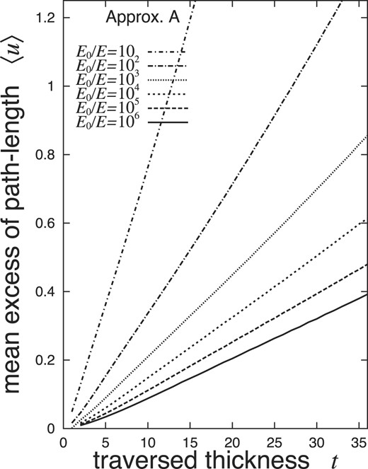
Mean EPL 〈u〉 under Approximation A for shower electrons, with a threshold energy of E and |$u \equiv 2E^2 \Delta /E_{\rm s}^2$|. Values of 〈u〉 are determined by the age |$\bar{s}$|, derived from Eq. (12) irrespective of the incident particle.
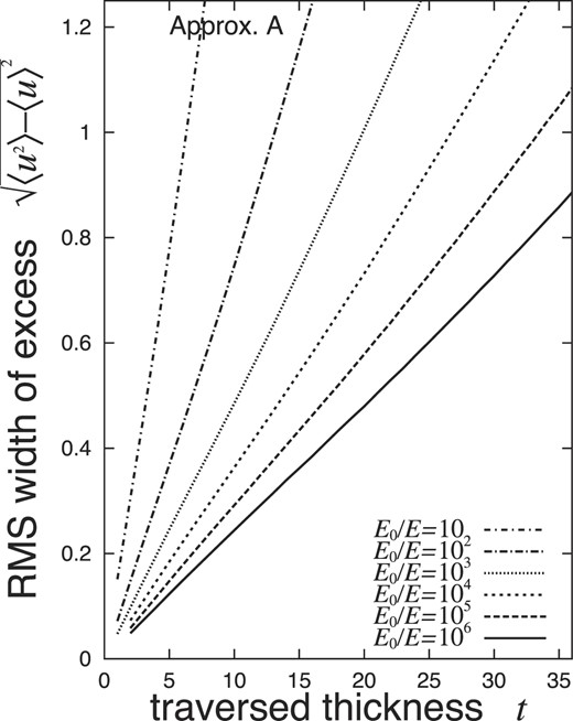
Root-mean-square EPL |$\sqrt{\langle u^2 \rangle - \langle u \rangle ^2}$| under Approximation A for shower electrons, with a threshold energy of E and |$u \equiv 2E^2 \Delta /E_{\rm s}^2$|. Values of |$\sqrt{\langle u^2 \rangle - \langle u \rangle ^2}$| are determined by the age |$\bar{s}$|, derived from Eq. (12) irrespective of the incident particle.
2.3. EPL distribution for shower electrons under Approximation A
The mean kth moments 〈Δk〉 or 〈uk〉 of Eq. (13) or (14) for the EPL distribution of shower electrons are special results of the Mellin transform with the transform variable κ at integer k. So, we can obtain the EPL distribution or the probability density for EPL from our Mellin transform 〈Δκ〉 or 〈uκ〉 of the generalized mean κth moment, extended from integer k to real κ.
We get our 〈Δκ〉 or 〈uκ〉 by interpolating |$\ln \left\lbrace {\phi _0^{(k)}(\bar{s};\lambda )}/{\phi _{00}(\bar{s};\lambda )}\right\rbrace _{\lambda \rightarrow \lambda _1(\bar{s})}$| at k = 0, 1, 2, 3, and 4 indicated in Table 1 with a quartic function:
as indicated in Fig. 3 and Table 3 for |$\bar{s} =$| 0.6, 1.0, 1.4, and 2.0. Then, applying the inverse Mellin transform on our 〈Δκ〉 or 〈uκ〉, we have the Δ- or u-weighted probability density of
where PA(E0, E, Δ, t) or |$p_{\rm A}(u,\bar{s})$| denotes the probability of shower electrons with energies greater than E to show their EPL smaller than Δ or u, satisfying
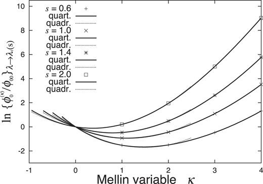
Interpolation of |$\ln \lbrace \phi _0^{(k)}(s;\lambda )/\phi _{00}(s;\lambda )\rbrace _{\lambda \rightarrow \lambda _1(s)}$| by the quartic functions of |$f(\kappa ) \equiv \sum _{j=1}^4 f_j \kappa ^j$| (thick lines) from dots at k = 0, 1, ⋅⋅⋅, and 4 and by the quadratic functions of f(κ) = f1κ + f2κ2 (thin lines) from dots at k = 0, 1, 2.
Interpolation of |$\ln \lbrace \phi _0^{(k)}(\bar{s};\lambda )/\phi _{00}(\bar{s};\lambda )\rbrace$| with |${\lambda \rightarrow \lambda _1(\bar{s})}$| by the quartic function of |$f(\kappa ) \equiv \sum _{j=1}^4 f_j \kappa ^j$|.
| |$\bar{s}$| | |$\ln \frac{\phi _0^{(1)}(\bar{s};\lambda )}{\phi _{00}(\bar{s};\lambda )}$| | |$\ln \frac{\phi _0^{(2)}(\bar{s};\lambda )}{\phi _{00}(\bar{s};\lambda )}$| | |$\ln \frac{\phi _0^{(3)}(\bar{s};\lambda )}{\phi _{00}(\bar{s};\lambda )}$| | |$\ln \frac{\phi _0^{(4)}(\bar{s};\lambda )}{\phi _{00}(\bar{s};\lambda )}$| | f1 | f2 | f3 | f4 |
|---|---|---|---|---|---|---|---|---|
| 0.6 | −1.528 | −1.501 | −0.470 | 1.316 | −2.565 | 1.192 | −0.1677 | 0.012 63 |
| 1.0 | −0.933 | −0.437 | 1.096 | 3.511 | −1.838 | 1.019 | −0.1245 | 0.009 85 |
| 1.4 | −0.472 | 0.480 | 2.612 | 5.762 | −1.286 | 0.871 | −0.0612 | 0.003 42 |
| 2.0 | 0.201 | 1.950 | 5.005 | 9.031 | −0.628 | 0.851 | −0.0171 | −0.003 85 |
The u-weighted probability density (17) can be evaluated as
by the saddle-point method, where the saddle point |$\bar{\kappa }$| is taken at |$-\bar{s}/2 \lt \bar{\kappa }$|. The density approaches
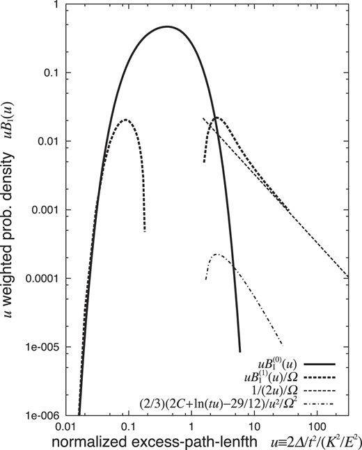
in the case of u ≪ 1, due to the residue of the pole at |$\kappa = -\bar{s}/2$|. We indicate these results in Fig. 4 for |$\bar{s} =$| 0.6, 1.0, 1.4, and 2.0.
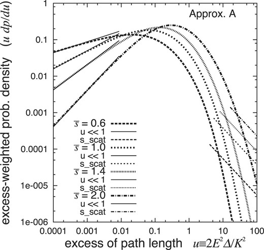
Probability densities of EPL for shower electrons under Approximation A at |$\bar{s}$| = 0.6, 1.0, 1.4, 2.0 (thick lines) and those at u ≪ 1 (thin solid lines), together with those determined by the Rutherford single scatterings (thin straight lines). The results depend on the incident particle only through the age |$\bar{s}$|.
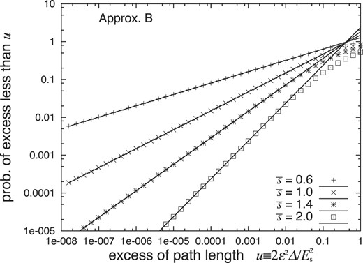
There remains an ambiguity in our evaluation of the EPL distribution due to the saddle point being taken as |$-\bar{s}/2 \lt \bar{\kappa }$|, which exceeds the interpolated region of |$\bar{\kappa }$| between 0 and 4 for |$f(\bar{\kappa })$| of Eq. (16). The residue at |$\kappa = -\bar{s}/2$| gives the probability densities |$dp_{\rm A}(u,\bar{s})/du$| with the power function of |$u^{\bar{s}/2-1}$| at the shower front of u ≪ 1 as indicated in Eq. (21); consequently it gives the corresponding probabilities |$p_{\rm A}(u,\bar{s})$| with the power function of |$u^{\bar{s}/2}$|. We compared these probabilities |$p_{\rm A}(u,\bar{s})$| with those obtained by the complex integration carried out numerically with the real part of κ within the interpolated region 0 < κ < 4 of f(κ), as described in Appendix B.1. Both agreed very well as indicated in Fig. 5; thus we find that |$f(\bar{\kappa })$| is sufficiently reliable in the extrapolated region of |$\bar{\kappa }$| up to |$-\bar{s}/2$|.
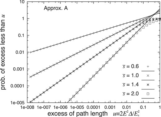
The probabilities |$p_{\rm A}(u,\bar{s})$| for shower electrons above the threshold energy of E with EPL up to u derived by the complex integral within the interpolated region of f(κ) (dots), compared with those derived by the residues at |$\kappa =-\bar{s}/2$| with f(κ) extrapolated (lines). The results depend on the incident particle only through the age |$\bar{s}$|.
Note that dpA/du is a function of only the age |$\bar{s}$|, slightly depending on the incident particle through the corresponding age |$\bar{s}$|.
3. The EPL distribution of cascade-shower electrons under Approximation B
3.1. The diffusion equation under Approximation B
We take into account the ionization loss of electrons under Approximation B, whence shower electrons lose their energies of εdt with the critical energy of ε in each infinitesimal traverse of dt [1,2]. Thus we have a diffusion equation for the EPL distribution:
under the Landau approximation. Then f(E, ζ, κ, λ) and g(E, ζ, κ, λ) defined in Eq. (2) satisfy
We express f and g by series expansion of
and then Eq. (23) becomes
Thus multiplying the inverse matrix Rs + 2κ + 2m of Eq. (6) to Eq. (25), we have a difference equation:
We solve this equation under Approximation B by introducing the factors of |$K_m^{(k)}(s,\nu )$| and |$H_m^{(k)}(s,\nu )$| to multiply the solutions of |$\phi _m^{(k)}(s;\lambda )$| under Approximation A as
Then we have a difference equation for |$K_m^{(k)}(s,\nu )$| and |$H_m^{(k)}(s,\nu )$| as
where we have introduced the operator ρ for the function of s as
Note that |$K_m^{(k)}(s,\nu )$| and |$H_m^{(k)}(s,\nu )$| also depend on λ.
3.2. Derivation of Km(k)(s, ν) with k = m = 0
We have a difference equation for |$K_0^{(0)}(s,\nu )$| from Eq. (28) as
which is a homogeneous difference equation indicated in Appendix A.2. As |$\phi _0^{(0)}(s,0;\lambda )$| gives the solution |$\phi _0^{(0)}(s;\lambda )$| under Approximation A, it satisfies |$K_0^{(0)}(s,0)=1$|. Thus according to Eq. (A5), we have the solution of
For ν of negative integer −n, the homogeneous solution (31) becomes expressed as
wherein the product of Γ(−n + 1)Ds shows indefinite at λ → λ1(s) evaluated as
Thus we have
3.3. Derivation of Km(k)(s, ν) with k + m = 1
3.3.1. The solution of K0(1)(s, ν).
The equations of |$K_{1-k}^{(k)}(s,\nu )$| and |$H_{1-k}^{(k)}(s,\nu )$| for k of 0 and 1 are derived from Eq. (28) as
where we have applied the relation of |$K_1^{(0)}(s,\nu )/H_1^{(0)}(s,\nu )=\hat{v}/\check{v}_{s+2+\nu }$| indicated in Eq. (35).
The homogeneous equations of |$\bar{K}_{1-k}^{(k)}(s,\nu )$| with the right-hand sides of Eqs. (35) and (36) set to 0 give the common solution of
to both equations, with |$\bar{K}_{1-k}^{(k)}(s,0) = 1$| applied at ν = 0. Then dividing Eqs. (35) and (36) with |$\bar{K}_{1-k}^{(k)}(s,\nu )$|, we have the equations for the relative solution |$\dot{K}_{1-k}^{(k)}(s,\nu ) \equiv K_{1-k}^{(k)}(s,\nu )/\bar{K}_{1-k}^{(k)}(s,\nu )$| with k of 0 and 1,
where we have introduced a function of
and applied the relation of
Thus applying Eq. (A2), we have the relative solutions as
Note that the operator Δν + 1 is applied to the variable i in the target function.
3.3.2. The solutions of K0(1)(s, ν) with ν of negative integer −n
For ν of negative integer −n, the homogeneous solutions (37) become expressed as
Γ(−n + 1) diverges, although the product with Ds appearing at n ≥ 3 gives the limiting value of Eq. (33) at λ → λ1(s). Thus we have
The relative solutions (42) and (43) for k = 0, 1 become expressed as
for ν of negative integer −n. |$\dot{K}_1^{(0)}(s,-n)$| of Eq. (46) shows the sum of n − 1 components valuable for n ≥ 2, where the first component (i = 1) is proportional to Ds. However, |$\dot{K}_0^{(1)}(s,-n)$| in Eq. (47) shows the sum of n − 2 components valuable for n ≥ 3, as |$\dot{K}_1^{(0)}(s,-i)$| in the first component (i = 1) vanishes as evaluated by Eq. (42), so that it starts from the second component (i = 2) of
where the function of s is conventionally expressed by the suffix of s, e.g. (BC)s instead of B(s)C(s).
3.4. Derivation of Km(k)(s, ν) with k + m = 2
3.4.1. The solution of K0(2)(s, ν)
The equations of |$K_{2-k}^{(k)}(s,\nu )$| and |$H_{2-k}^{(k)}(s,\nu )$| for k of 0, 1, and 2 are derived from Eq. (28) as
The homogeneous equations of |$\bar{K}_{2-k}^{(k)}(s,\nu )$| with the right-hand sides of Eqs. (49), (50), and (51) set to 0 give the common solution of
to those equations, with |$\bar{K}_{2-k}^{(k)}(s,0) = 1$| applied at ν = 0.
Then the relative solutions |$\dot{K}_{2-k}^{(k)}(s,\nu ) \equiv K_{2-k}^{(k)}(s,\nu )/\bar{K}_{2-k}^{(k)}(s,\nu )$| satisfy the following equations:
where we have applied the relation of
and substituted into Eq. (55) the term
which is derived from the electron- and photon-side equations in Eq. (50). Thus the relative solutions are expressed as
due to Eq. (A2) for f(0) = ψ(0).
3.4.2. The solutions of K0(2)(s, ν) with ν of negative integer −n
For ν of negative integer −n, the homogeneous solutions (52) become expressed as
The product of Γ(−n + 1) and Ds appearing at n ≥ 5 gives the limiting value of Eq. (33) at λ → λ1(s). Thus we have
The relative solution (58) for k = 0 becomes expressed as
where the component of summation at i = 1 does not contribute as |$\dot{K}_1^{(0)}(s,-1) = 0$|, the components at i = 2, 3 contribute infinitesimally due to Ds at λ → λ1(s) as
and the components at i ≥ 4 contribute by finite terms. Thus we find that |$\dot{K}_2^{(0)}(s,-n)$| gives 0 for n ≤ 2, an infinitesimal value for n = 3, 4, and the sum of n − 4 finite components starting with i = 4 for n ≥ 5.
The relative solution (59) for k = 1 becomes expressed as
where the components of summation do not contribute at i = 1, 2 as |$\dot{K}_0^{(1)}(s,-j) = 0$| and |$\dot{K}_2^{(0)}(s,-j) = 0$|, the component at i = 3 contributes infinitesimally as ρ−3Ds + 3 and |$\dot{K}_2^{(0)}(s,-3)$| is infinitesimal due to Ds at λ → λ1(s), and the components at i ≥ 4 contribute by finite terms. Note that the second term of the component at i = 4 has Ds, but is reduced to a finite term as
Thus we find that |$\dot{K}_1^{(1)}(s,-n)$| gives 0 for n ≤ 3, an infinitesimal value for n = 4, and the sum of n − 4 finite components starting with i = 4 for n ≥ 5.
The relative solution (60) for k = 2 becomes expressed as
where the components of summation at i = 1, 2 vanish as the terms |$\dot{K}_1^{(1)}(s,-i)$| and |$\dot{K}_2^{(0)}(s,-i)$| are both 0, the component at i = 3 does not contribute as |$\dot{K}_1^{(1)}(s,-3)$| and |$\dot{K}_2^{(0)}(s,-3)$| are 0 and infinitesimal, and the components at i ≥ 4 contribute by finite terms, though the component at i = 4 is expressed as
after reducing the Ds in the numerator and the denominator. Thus we find that |$\dot{K}_0^{(2)}(s,-n)$| gives 0 for n ≤ 3, an infinitesimal value for n = 4, and the sum of n − 4 finite components starting with i = 4 for n ≥ 5.
3.5. The kth moment of the EPL distribution for shower electrons under Approximation B
3.5.1. The kth moment of the EPL distribution for total shower electrons
Let |$\Pi _{\rm B}^{(k)}(E_0,E,t)$| be the kth moment of EPL distribution under Approximation B for shower electrons of energies greater than E at the traversed thickness of t, with the angular distribution integrated. We have, from f(E, ζ, κ, λ) of Eq. (2) with Eq. (24),
where ε denotes the critical energy indicated in Refs. [1,2] and |$\phi _0^{(k)}(s,\nu ;\lambda )$| is replaced by |$\phi _0^{(k)}(s;\lambda )$| and |$K_0^{(k)}(s,\nu )$| with Eq. (27). For the “total” shower electrons (the threshold energy E of 0), the integration with ν is replaced by the residue at the pole of ν = −s − 2k. Thus we have
where the complex integration with λ is evaluated approximately by the residue from the pole at λ = λ1(s).
In particular, for k = 0, |$\Pi _{\rm B}^{(k)}(E_0,0,t)$| gives the total number of electrons (E → 0) under Approximation B evaluated as
by the saddle-point method [1,2], with a conventional saddle point |$\bar{s}$| determined by
irrespective of the incident particle, where ΠA(E0, ε, t) and |$\bar{s}$| are determined by Eqs. (11) and (12) with E replaced by ε. The saddle point |$\bar{s}$| is called the shower age under Approximation B. Note that |$\bar{s}$| under Approximation B for photon-incident showers can also be slightly improved [1] as |$\bar{s}$| under Approximation A (see footnote 2), expecting a better saddle point.
|$\lbrace K_0^{(0)}(\bar{s},-\bar{s})\rbrace _{\lambda \rightarrow \lambda _1(\bar{s})}$| for non-integer |$\bar{s}$| is evaluated by Eq. (31), and those for integer |$\bar{s}$| are evaluated by Eq. (34) exactly without converging ambiguities as indicated in Table 5 for |$\bar{s} =$| 1, 2, ⋅⋅⋅, and 5. Those for non-integer and integer |$\bar{s}$| are shown by dots in Fig. 6, which are already indicated in Refs. [1,2]. We express the function of |$\ln \lbrace K_0^{(0)}(\bar{s},-\bar{s})\rbrace _{\lambda \rightarrow \lambda _1(\bar{s})}$| explicitly in a quartic polynomial,
by interpolating the values of those at |$\bar{s} =$| 0, 1, 2, ⋅⋅⋅, and 5, as shown by lines in Fig. 6.
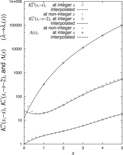
|$K_0^{(0)}(s,-s)$|, |$K_0^{(1)}(s,-s-2)$|, and Λ(s) with λ → λ1(s) at integer s of 1, 2, ⋅⋅⋅, and 5 (○) and non-integer s (+), as well as the approximated quartic functions from those at integer s (lines).
Then we have the mean kth moment of EPL distribution averaged over total shower electrons as
where we have introduced a new normalized variable of
for the EPL under Approximation B.
3.5.2. The mean first moment of the EPL distribution averaged over total shower electrons
The mean EPL for shower electrons requires
as expressed in Eq. (76) with k = 1, where
are derived from Eqs. (37) and (43). So |$\lbrace K_0^{(1)}(\bar{s},-\bar{s}-2)\rbrace _{\lambda \rightarrow \lambda _1(\bar{s})}$| for non-integer |$\bar{s}$| are evaluated, as shown by dots in Fig. 6. However, those for integer |$\bar{s}$| are solved from Eqs. (44) and (47) exactly without converging ambiguities, in which the relative solutions are indicated in Table 4. Thus those with |$\lambda \rightarrow \lambda _1(\bar{s})$| are evaluated as indicated in Table 5, in which |$\lbrace K_0^{(1)}(\bar{s},-\bar{s}-2)\rbrace _{\lambda \rightarrow \lambda _1(\bar{s})}$| are evaluated for integer |$\bar{s}$| of 1, 2, ⋅⋅⋅, and 5, as shown by dots in Fig. 6. We express the function of |$\ln \lbrace K_0^{(1)}(\bar{s},-\bar{s}-2)\rbrace _{\lambda \rightarrow \lambda _1(\bar{s})}$| explicitly in a quartic polynomial,
by interpolating the values of those at |$\bar{s} =$| 1, 2, ⋅⋅⋅, and 5, as shown by lines in Fig. 6. The interpolated formula (81) seems sufficiently applicable even at |$0.6 \lesssim \bar{s}$|, within the converging ambiguities of Eq. (80).
|$\dot{K}_0^{(1)}(j,-j-2)$| up to j = 5.
| j | |$\dot{K}_0^{(1)}(j,-j-2)$| |
|---|---|
| 1 | |$\dot{K}_0^{(1)}(1,-3) = \frac{3\times 2}{D_2\hat{v}_{3}^{(1)}}\frac{\hat{v}^2+(BC)_{1}}{2\times 1}$| |
| 2 | |$\dot{K}_0^{(1)}(2,-4) = \frac{4\times 3}{D_3\hat{v}_{4}^{(1)}}\left\lbrace \frac{\hat{v}^2+(BC)_{2}}{3\times 2}+\frac{\hat{v}^2+(BC)_{1}}{2\times 1}\right\rbrace$| |
| 3 | |$\dot{K}_0^{(1)}(3,-5) = \frac{5\times 4}{D_4\hat{v}_{5}^{(1)}}\left\lbrace \frac{\hat{v}^2+(BC)_{3}}{4\times 3}+\frac{\hat{v}^2+(BC)_{2}}{3\times 2}+\frac{\hat{v}^2+(BC)_{1}}{2\times 1}\left(1+\frac{D_2}{3D_1}\right)\right\rbrace$| |
| 4 | |$\dot{K}_0^{(1)}(4,-6) = \frac{6\times 5}{D_5\hat{v}_{6}^{(1)}}\left\lbrace \frac{\hat{v}^2+(BC)_{4}}{5\times 4}+\frac{\hat{v}^2+(BC)_{3}}{4\times 3} +\frac{\hat{v}^2+(BC)_{2}}{3\times 2}\left(1+\frac{D_3}{2D_2}\right) + \frac{\hat{v}^2+(BC)_{1}}{2\times 1}\left(1+\frac{D_2}{3D_1}+\frac{D_3}{6D_1}\right)\right\rbrace$| |
| 5 | |$\dot{K}_0^{(1)}(5,-7) = \frac{7\times 6}{D_6\hat{v}_{7}^{(1)}}\left\lbrace \frac{\hat{v}^2+(BC)_{5}}{6\times 5}+\frac{\hat{v}^2+(BC)_{4}}{5\times 4} +\frac{\hat{v}^2+(BC)_{3}}{4\times 3}\left(1+\frac{3D_4}{5D_3}\right) \,\,\,\, \right.$| |
| |$\left. +\frac{\hat{v}^2+(BC)_{2}}{3\times 2}\left(1+\frac{D_3}{2D_2}+\frac{3D_4}{10D_2}\right) +\frac{\hat{v}^2+(BC)_{1}}{2\times 1}\left(D_1+\frac{D_2}{3}+\frac{D_3}{6}+\frac{D_4}{10}\right)\right\rbrace$| |
|$K_0^{(0)}(\bar{s},-\bar{s})$|, |$\bar{K}_0^{(1)}(\bar{s},-\bar{s}-2)$|, |$\dot{K}_0^{(1)}(\bar{s},-\bar{s}-2)$|, |$K_0^{(1)}(\bar{s},-\bar{s}-2)$|, |$\bar{K}_0^{(2)}(\bar{s},-\bar{s}-4)$|, |$\dot{\Lambda }(\bar{s})$|, and |$\Lambda (\bar{s})$| with |$\lambda \rightarrow \lambda _1(\bar{s})$| at |$\bar{s}$| of integer values up to 5.
| |$\bar{s}$| | |$K_0^{(0)}$| | |$\bar{K}_0^{(1)}$| | |$\dot{K}_0^{(1)}$| | |$K_0^{(1)}$| | |$\bar{K}_0^{(2)}$| | |$\dot{\Lambda }$| | Λ |
|---|---|---|---|---|---|---|---|
| 1 | 2.29 | 2.461 | 8.20 | 20.5 | 1.03 × 100 | 3.18 × 10² | 3.27 × 10² |
| 2 | 3.45 | 0.691 | 63.50 | 43.9 | 1.16 × 10⁻¹ | 2.25 × 10⁴ | 2.61 × 10³ |
| 3 | 5.98 | 0.484 | 243.78 | 117.9 | 4.79 × 10⁻² | 2.36 × 10⁵ | 1.13 × 10⁴ |
| 4 | 10.62 | 0.449 | 597.50 | 268.3 | 2.98 × 10⁻² | 1.24 × 10⁶ | 3.69 × 10⁴ |
| 5 | 18.08 | 0.454 | 1192.32 | 540.9 | 2.13 × 10⁻² | 4.65 × 10⁶ | 9.90 × 10⁴ |
The results of the mean EPL |$\langle u \rangle \equiv 2\varepsilon ^2 \langle \Delta \rangle / E_{\rm s}^2$| for total shower electrons expressed by Eq. (76) with k = 1 are evaluated by applying the contents of Table 1 and Eqs. (74) and (81), as indicated in Fig. 7 for E0/ε = 10, 102, ⋅⋅⋅, and 106 (lines). Note that 〈u〉 is a function of only the age |$\bar{s}$|, slightly depending on the incident particle through the corresponding age |$\bar{s}$|.
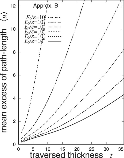
Mean EPL 〈u〉 under Approximation B for shower electrons, with the threshold energy E of 0 and |$u \equiv 2\varepsilon ^2 \Delta /E_{\rm s}^2$|. Values of 〈u〉 are determined by the age s, derived from Eq. (73) irrespective of the incident particle.
3.5.3. The mean second moment of the EPL distribution averaged over total shower electrons
The mean second moment of the EPL distribution for total shower electrons, expressed in Eq. (76) with k = 2, requires
At s of integer 1, |$\bar{K}_0^{(2)}(1,-5)$| is finite as derived from Eq. (62). However, |$\dot{K}_0^{(2)}(s,-5)$| diverges at s → 1 due to the pole of second degree at s = 1, by the term of ρ−2DSSs + 1 in Eq. (69). Thus the mean second moment 〈Δ2〉 and hence the root-mean-square width |$\sqrt{\langle \Delta ^2 \rangle -\langle \Delta \rangle ^2}$| of the EPL distribution for total shower electrons diverge at s = 1. At s of integer 2, |$\bar{K}_0^{(2)}(2,-6)$| is finite as derived from Eq. (62). However, |$\dot{K}_0^{(2)}(s,-6)$|, requiring |$\dot{K}_2^{(0)}(s,-5)$| and |$\dot{K}_1^{(0)}(s,-4)$| at Eqs. (68) and (63), diverges at s → 2 due to the pole of second degree at s = 2, by the term of ρ−3DSSs + 1 appearing at i = 3 of the summation in |$\dot{K}_1^{(0)}(s,-4)$| of Eq. (46). Thus 〈Δ2〉 and hence |$\sqrt{\langle \Delta ^2 \rangle -\langle \Delta \rangle ^2}$| diverge at s = 2. In the same way, 〈Δ2〉 and hence |$\sqrt{\langle \Delta ^2 \rangle -\langle \Delta \rangle ^2}$| diverge at s → 3, 4, ⋅⋅⋅, due to the pole of second degree at s = 3, 4, ⋅⋅⋅.
At s of non-integer values, |$\bar{K}_0^{(2)}(s,-s-4)$| is finite as derived from Eq. (52). However, |$\dot{K}_0^{(2)}(s^{\prime },-s-4)$| of Eq. (60), requiring |$\dot{K}_2^{(0)}(s^{\prime },-s-3)$| and hence |$\dot{K}_1^{(0)}(s^{\prime },-s-2)$| of Eqs. (58) and (42), diverges at s′ → s due to the pole of second degree at s′ = s by the term of |$\Delta _{-s-1}{\rm DSS}_{s^{\prime }+1}$| appearing in |$\dot{K}_1^{(0)}(s^{\prime },-s-2)$| at i = 0 of the summation. Thus, 〈Δ2〉 and hence |$\sqrt{\langle \Delta ^2 \rangle -\langle \Delta \rangle ^2}$| diverge for s of non-integer values, due to the pole of second degree at s′ = s.
Evaluating the mean moments of shower electrons with their threshold energy of E finite (E > 0), 〈Δ〉, 〈Δ2〉 and hence |$\sqrt{\langle \Delta ^2 \rangle -\langle \Delta \rangle ^2}$| do not diverge, as the moments of individual electrons in the shower do not diverge due to the finite threshold of energy [5,11]. Linsley and Scarsi regarded the thickness of the shower front as an effective observable for quantitative analyses of extensive air shower [6]. However, it should be noted that 〈Δ2〉 and hence |$\sqrt{\langle \Delta ^2 \rangle -\langle \Delta \rangle ^2}$| are very sensitive to the value of the threshold energy E.
3.6. EPL distribution for shower electrons under Approximation B
3.6.1. Our Mellin transform of 〈Δκ〉 or 〈uκ〉 under Approximation B
We derive our Mellin transform 〈Δκ〉 or 〈uκ〉 of the generalized mean κth moment by extending the mean kth moment 〈Δk〉 or 〈uk〉 of Eq. (75) or (76) for integer k to that for real κ.
We investigate first the analytical property of |${K}_0^{(\kappa )}(s,-s-4)$| at κ → 2. As confirmed in Section 3.5.3, |$\dot{K}_0^{(2)}(s,\nu )$| diverges at ν → −s − 4 due to the pole of the second degree. So |$\lbrace (s+2\kappa +\nu )^2 \dot{K}_0^{(\kappa )}(s,\nu )\rbrace _{\kappa = 2}$| gives a finite limiting value at ν → −s − 4. As |$\dot{K}_0^{(\kappa )}(s,\nu )$| is continuous with κ and ν, |$\lbrace (s+2\kappa +\nu )^2 \dot{K}_0^{(\kappa )}(s,\nu )\rbrace _{\nu = -s-4}$| also gives the same limiting value at κ → 2:
where the limiting values of |$\dot{\Lambda }(s)$| and Λ(s) are defined. |$\dot{\Lambda }(j)$| for j of positive integer is derived by applying the solution of |$\dot{K}_0^{(2)}(s,-n)$| indicated in Eq. (68) as
where we have applied lims → j(s − j)2DSSs − j = −1.36B(0). Thus |$\dot{\Lambda }(\bar{s})$| and |$\Lambda (\bar{s})$| of Eqs. (83) and (84) with |$\lambda \rightarrow \lambda _1(\bar{s})$| are evaluated for |$\bar{s} =$| 1, 2, ⋅⋅⋅, and 5, as indicated in Table 5 and shown by dots in Fig. 6. We express the function of |$\ln \lbrace \Lambda (\bar{s})\rbrace _{\lambda \rightarrow \lambda _1(\bar{s})}$| explicitly in a quartic polynomial,
by interpolating the values of those at |$\bar{s} =$| 1, 2, ⋅⋅⋅, and 5, as shown by lines in Fig. 6.
Then, we express |$\ln \lbrace \phi _0^{(\kappa )}(\bar{s};\lambda )/\phi _{00}(\bar{s};\lambda )\rbrace _{\lambda \rightarrow \lambda _1(\bar{s})}$| by a quadratic function of κ satisfying those indicated in Table 1 at κ = 0, 1, 2, under Approximation B:
where f(κ) determined here shows a negligible difference from f(κ) of Eq. (16) under Approximation A in the applicable region of |$-\bar{s}/2 \lt \bar{\kappa } \lt 2$|, as compared in Fig. 3. On the other hand we express |$\ln \lbrace (\kappa -2)^2K_0^{(\kappa )}(\bar{s},-\bar{s}-2\kappa )/(4 K_0^{(0)}(\bar{s},-\bar{s}))\rbrace _{\lambda \rightarrow \lambda _1(\bar{s})}$| by a quadratic function of κ satisfying those at κ = 0, 1, 2, applying the limiting value |$\Lambda (\bar{s})$| of Eq. (84) at κ = 2:
Thus we have our Mellin transform 〈uκ〉 of
The coefficients of f1, f2, g1, and g2 determined here are indicated in Table 6 and the |$\left\lbrace {K_0^{(\kappa )}(\bar{s},-\bar{s}-2\kappa )}/{K_0^{(0)}(\bar{s},-\bar{s})}\right\rbrace _{\lambda \rightarrow \lambda _1(\bar{s})}$| values are indicated in Fig. 8, for |$\bar{s} =$| 0.6, 1.0, 1.4, and 2.0.
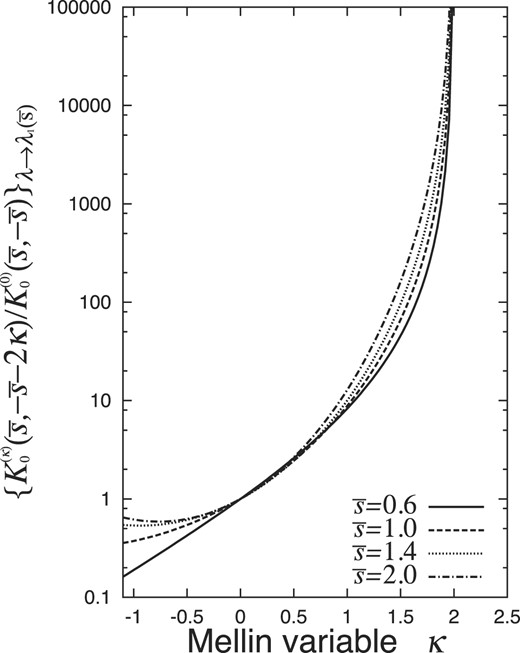
Our approximated functions of |$K_0^{(\kappa )}(\bar{s},-\bar{s}-2\kappa )/K_0^{(0)}(\bar{s},-\bar{s})$| with |$\lambda \rightarrow \lambda _1(\bar{s})$| for |$\bar{s} =$| 0.6, 1.0, 1.4, and 2.0.
Interpolation of |$\ln \lbrace \phi _0^{(k)}(\bar{s};\lambda )/\phi _{00}(\bar{s};\lambda )\rbrace _{\lambda \rightarrow \lambda _1(s)}$| and |$\ln \lbrace \lbrace K_0^{(\kappa )}(\bar{s},-\bar{s}-2\kappa )/K_0^{(0)}(\bar{s},-\bar{s})\rbrace \rbrace _{\lambda \rightarrow \lambda _1(s)}$| by the quadratic functions of f1κ + f2κ2 and g1κ + g2κ2.
| |$\bar{s}$| | f1 | f2 | g1 | g2 |
|---|---|---|---|---|
| 0.6 | −2.306 | 0.778 | 0.791 | −0.0623 |
| 1.0 | −1.649 | 0.715 | 0.483 | 0.3095 |
| 1.4 | −1.184 | 0.712 | 0.365 | 0.5533 |
| 2.0 | −0.572 | 0.774 | 0.419 | 0.7470 |
| |$\bar{s}$| | f1 | f2 | g1 | g2 |
|---|---|---|---|---|
| 0.6 | −2.306 | 0.778 | 0.791 | −0.0623 |
| 1.0 | −1.649 | 0.715 | 0.483 | 0.3095 |
| 1.4 | −1.184 | 0.712 | 0.365 | 0.5533 |
| 2.0 | −0.572 | 0.774 | 0.419 | 0.7470 |
3.6.2. Probability density of EPL for total shower electrons
By applying the inverse Mellin transform on our 〈uκ〉 of Eq. (91), we have the Δ- or u-weighted probability density of
where PB(E0, 0, Δ, t) or |$p_{\rm B}(u,\bar{s})$| denotes the probability for total shower electrons (the threshold energy E of 0) to show their EPL smaller than Δ or u, satisfying
The u-weighted probability density (92) can be evaluated as
by the saddle-point method, where the saddle point |$\bar{\kappa }$| is taken at |$-\bar{s}/2 \lt \bar{\kappa } \lt 2$| satisfying
In particular, in the case of u ≪ 1 or u ≫ 1, the density approaches
due to the residue of the pole at |$\kappa = -\bar{s}/2$| or κ = 2. These results for |$\bar{s} =$| 0.6, 1.0, 1.4, and 2.0 are indicated in Fig. 9.
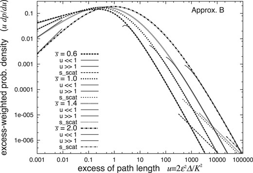
Probability densities of EPL for shower electrons under Approximation B at |$\bar{s}$| = 0.6, 1.0, 1.4, 2.0 (thick lines) and those at u ≪ 1 and u ≫ 1 (thin solid lines), together with those determined by the Rutherford single scatterings (thin straight lines). The results depend on the incident particle only through the age |$\bar{s}$|.
Our |$f(\bar{\kappa })$| and |$g(\bar{\kappa })$| of Eqs. (87) and (89) under Approximation B are also sufficiently reliable in the extrapolated region of |$\bar{\kappa }$| up to |$-\bar{s}/2$|, as under Approximation A. We have confirmed in Appendix B.2 that the results of |$p_{\rm B}(u,\bar{s})$| at u ≪ 1 derived from our extrapolated |$f(\bar{\kappa })$| and |$g(\bar{\kappa })$| at |$\bar{\kappa } = -\bar{s}/2$| agree very well with those derived by the complex integration carried out numerically in the interpolated region of f(κ) and g(κ) with the real part of κ between 0 and 2, as indicated in Fig. 10.
The probabilities |$p_{\rm B}(u,\bar{s})$| for shower electrons above the threshold energy E of 0 with EPL up to u derived by the complex integral within the interpolated region of f(κ) and g(κ) (dots), compared with those derived by the residues at |$\kappa =-\bar{s}/2$| with f(κ) and g(κ) extrapolated (lines). The results depend on the incident particle only through the age |$\bar{s}$|.
Our analytical results (94) of EPL distribution are compared in Fig. 11 with those derived by a Monte Carlo method [12,13] based on the Yang formulae [4,5], for showers with an incident energy E0 of 104ε and a threshold energy E of 0 (in the former) or 0.01ε (in the latter) at t = 5, 10, 15, 20, and 25 (thus |$\bar{s}$| = 0.735, 1.12, 1.38, 1.50, and 1.75). They both agreed fairly well, in spite of the difference of the threshold energies E between them.
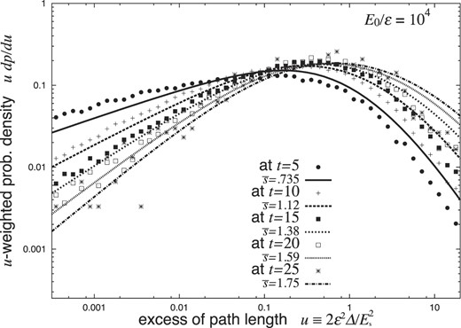
Our EPL probability densities for shower electrons with an incident energy E0 of 104ε and a threshold energy E of 0 at t = 5, 10, 15, 20, 25 or |$\bar{s}$| = 0.735, 1.12, 1.38, 1.50, 1.75 (thick lines), compared with those derived by 100 photon-induced Monte Carlo showers with E0 of 104ε and E of 0.01 ε (dots).
As we found in Eq. (96), the probability density dpB/du decreases with the power function of |$u^{\bar{s}/2-1}$| at the shower front of u ≪ 1, for showers with the age of |$\bar{s}\lt 2$|. This fact is a characteristic property of a shower at an age |$\bar{s}$| comparable with the fact that the lateral distribution of shower electrons decreases with |$(\varepsilon ^2 r^2/E_{\rm s}^2)^{\bar{s}/2-1}$| near the shower axis of r ≪ Es/ε [2,3], as discussed by Aglietta et al. [9] from the empirical point of view.
Note that dpB/du is a function of only the age |$\bar{s}$|, slightly depending on the incident particle through the corresponding age |$\bar{s}$|. It should also be noted that udpB/du can be well observed at radial distances of r from the shower axis, with only its starting part lacking as indicated in Fig. 12 in the case of |$\bar{s}=1.0$| [14].
![Probability densities d2ρ/du/d(v/t) = $\pi r_{\rm M}^2 t d^2 \rho /du/d\vec{r}$ of EPL in the case of $\bar{s}=1.0$ with u2/h weighted, h = 9 set, and rM ≡ Es/ε of the Molière unit denoted [2,3], for shower electrons at traversed thickness of t and radial distances of r reflected in u0 ≡ v/t = (r/rM)2/t (dotted lines) [14]. They approach udp/du (thin solid line) at r → 0. The results depend on the incident particle only through the age $\bar{s}$.](https://oup.silverchair-cdn.com/oup/backfile/Content_public/Journal/ptep/2024/4/10.1093_ptep_ptae047/1/m_ptae047fig12.jpeg?Expires=1747998405&Signature=Ph3saGnGmMcc5WAdgpakw7XReOCrdBhVYB03rX5MOud7YvtwjMq3J5dkcdXpn7sWj~8lbPggoOI8ZJsfnj2GN~4U30MnO32i78wt-JTJ4irN32dkvWo7GvVRlARsy3mfHPJl5QzwjITqiekonYUYkS-MDiVrW1thLD3QB3rFV~DmZOjVpWSUO-HU~4Kb54Ajf2msBTLeqKQEdjKys2OYvyWrTW7tIiygHyf14~GZ9Z5XBXzj-dUaBm2acC81RS8U18K0iIFfHAOT61VyOR9l~boy-J-jCi5hSqfYIlJkj3EsxHtrsiDnoW79SrouLrjR0DbwsV8IvZ8HQKqOnKQE2Q__&Key-Pair-Id=APKAIE5G5CRDK6RD3PGA)
Probability densities d2ρ/du/d(v/t) = |$\pi r_{\rm M}^2 t d^2 \rho /du/d\vec{r}$| of EPL in the case of |$\bar{s}=1.0$| with u2/h weighted, h = 9 set, and rM ≡ Es/ε of the Molière unit denoted [2,3], for shower electrons at traversed thickness of t and radial distances of r reflected in u0 ≡ v/t = (r/rM)2/t (dotted lines) [14]. They approach udp/du (thin solid line) at r → 0. The results depend on the incident particle only through the age |$\bar{s}$|.
4. The EPL distribution of shower electrons due to Rutherford single scattering
We have to investigate the contributions of Rutherford single scattering in the EPL distribution in large excess regions, as investigated in the lateral distribution without the Landau approximation by Kamata and Nishimura [2,3]. We confirm in Appendix C that the large angle and the large EPL distributions of penetrating electrons can be well reproduced by the large-angle scattering σL of electrons assumed to penetrate straight before and after the single scattering, as indicated in Figs. 13 and 14. So we evaluate the large EPL distribution of shower electrons by applying Rutherford single scattering to the shower electrons, assuming shower particles to propagate straight toward the direction of shower development before and after the single scattering.
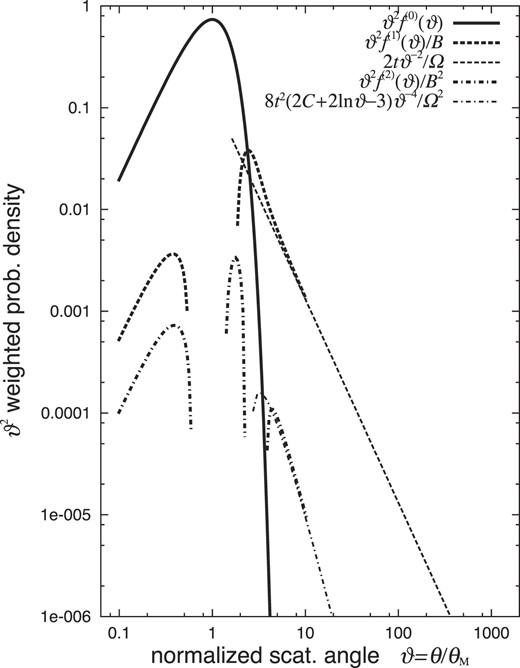
The first three terms (k = 0, 1, 2) of a Molière series for the angular distribution of the penetrating electrons at t = 1, compared with the contributions from the first large-angle scattering (k = 1) and the second (k = 2).
The first two terms (k = 0, 1) of a Molière series for the EPL distribution of the penetrating electrons at t = 1, compared with the contributions from the first large-angle scattering (k = 1) and the second (k = 2).
4.1. The distribution under Approximation A
As the scattered angle θ at t′ causes the EPL Δ at t by
the Rutherford scattering probability per g/cm2 for electrons of energy E′ at t′ [2,15] is transformed to the EPL distribution at t as [5]
where the constants K and Ω are defined in Kamata and Nishimura [2,3] and the infinitesimal traversed thickness dx′ in g/cm2 is exchanged to dt′ in units of radiation length. A cascade shower induced by photons of energy W0 produces a differential energy spectrum of
for electrons at t′ under Approximation A [1,2]. The respective electrons in the spectrum are multiplied by
at the destination thickness t with E of the threshold energy, after receiving Rutherford scattering only once at t′ during the passage from 0 to t. Thus the electrons in the spectrum (100) at t′ contribute to the EPL distribution at t by the single scattering of Eq. (99) as
Therefore, integrating Eq. (102) with t′ from 0 to t and dividing the result by the number of electrons ΠA(W0, E, t), we have the infinitesimal probability dPA(W0, E, Δ, t) for EPL to exceed Δ within dΔ. Then the Δ-weighted probability density for Δ at t is expressed as
We carried out this integration numerically. The factor QA(W0/E, t′) defined in Eq. (102) is evaluated by the double complex integral with p and q. In particular, for t′ of 0 and t, it satisfies
and for general t′ it is evaluated by the double saddle-point method [2] as
where the double saddle point |$(\bar{p},\bar{q})$| is determined by3
The resultant Δ-weighted probability densities (103) of the EPL due to the Rutherford single scattering are indicated in Fig. 4 (thin straight lines) with the normalized variable u of Eq. (15), compared with those results (17) derived under the Landau approximation (thick lines). We took W0/E = 6.32 × 10⁹, 54 600, 516, and 20.1 for t = 10 so as the shower age |$\bar{s}$| from Eq. (12) satisfied 0.6, 1.0, 1.4, and 2.0, and also we set Ω = 15.2 and did not distinguish K and Es. We find that the probability densities dPA/dΔ due to the Rutherford single scattering exceed those derived under the Landau approximation in very large EPL regions (100 times or more of the peak positions of the EPL-weighted probability density) with the densities decreasing with Δ−2.
4.2. The distribution under Approximation B
The differential energy spectrum for electrons at the traversed thickness t′ is expressed as
under Approximation B [1,2]. The EPL distribution of Eq. (99) caused by the Rutherford single scattering of electrons at t′ is affected in electrons at the destination thickness t, multiplied by
with E of the threshold energy. Thus the Rutherford single scattering of Eq. (99) at t′ contributes to the EPL distribution at t by
where we have defined QB(W0/E, t′) as
depending on QA(W0/ε, t′) of Eq. (105) with its double saddle point of |$(\bar{p},\bar{q})$|.
Integrating Eq. (109) with t′ from 0 to t and dividing the result by the number of electrons ΠB(W0, E, t), we have the infinitesimal probability dPB(W0, E, Δ, t) for EPL to exceed Δ within dΔ. Then the Δ-weighted probability density for Δ at t is expressed as
We carried out this integration numerically, as performed under Approximation A.
The resultant Δ-weighted probability densities (111) of the EPL due to the Rutherford single scattering are indicated in Fig. 9 (thin straight lines) with the normalized variable u of Eq. (77), compared with those results (92) derived under the Landau approximation (thick lines). We took W0/ε = 6.32 × 10⁹, 54 600, 516, and 20.1 for t = 10 so as the shower age |$\bar{s}$| from Eq. (73) satisfied 0.6, 1.0, 1.4, and 2.0, and also we set Ω = 15.2 and did not distinguish K and Es. We find that the probability densities dPB/dΔ due to the Rutherford single scattering exceed those derived under the Landau approximation in very large EPL regions (about 10 000 times or more of the peak positions of the PL-weighted probability density) with the densities decreasing with Δ−2.
5. Summary and discussions
EPL distributions for cascade-shower electrons were investigated first by proposing and solving a diffusion equation under the Landau approximation.
In cases in which ionization loss is not taken into account (Approximation A), the mean kth moments of the EPL distribution for shower electrons were solved up to the fourth. The mean and the root-mean-square width of the distribution were derived from those moments (Figs. 1 and 2). By moderately interpolating the ratio |${\phi _0^{(k)}}/{\phi _{00}}$| at k = 0, 1, 2, 3, and 4 (Fig. 3), we got our Mellin transform 〈uκ〉 of Eq. (16) possessing a pole at |$\kappa =-\bar{s}/2$|, from which we obtained the EPL distributions indicated in Fig. 4 (thick lines).
In cases in which ionization loss is taken into account (Approximation B), the mean moments of the EPL distribution for shower electrons were solved by further introducing the factor |$K_0^{(k)}(s,\nu )$| to multiply |$\phi _0^{(k)}(s;\lambda )$| under Approximation A. The mean EPL was derived from the first moment (Fig. 7), though the root-mean-square width could not be obtained due to divergence of the factor |$K_0^{(2)}$| with a pole of the second degree. By moderately interpolating the ratio |${K_0^{(k)}}/{K_0^{(0)}}$| at k = 0, 1, and 2 (Fig. 8), we got our Mellin transform 〈uκ〉 of Eq. (91) possessing poles at |$\kappa =-\bar{s}/2$| and 2, from which we obtained the EPL distributions indicated in Fig. 9 (thick lines).
The EPL distributions due to Rutherford single scattering were investigated next under Approximations A and B as indicated in Figs. 4 and 9 (thin straight lines); they decreased more slowly and showed higher probability densities in sufficiently large EPL regions than those derived under the Landau approximation in Sections 2 and 3. Since these effects appear in very large EPL regions, as shown in the figures, the EPL distributions observed up to around the peak positions of the EPL-weighted probability density could be well analyzed with the results under the Landau approximation.
The EPL distribution of shower electrons gives their longitudinal distribution observed as an arrival-time distribution at the given thickness of traverse, which will be equally as important as their lateral distribution for investigations of cascade showers developing in thin matter, e.g. in air. The present theory of EPL distribution will verify and improve traditional investigations of cascade showers, by appending other precise qualitative and quantitative analyses to those that the theory of lateral distribution has provided [2,3].
Conflict of interest statement. None declared.
Acknowledgement
The authors are very indebted to Prof. J. Nishimura for his valuable advice and encouragement. They also wish to express their great thanks to the members of Okayama Cosmic-Ray Simulation Group [14] for useful discussions about the content, as well as to Dr S. Tanaka for reading and improving the manuscript.
A. Solutions of the difference equation
A.1. Recurrence equation
The recurrence equation
is solved as
where we define
A.2. Homogeneous difference equation
The homogeneous difference equation
is solved as
A.3. Inhomogeneous difference equation
We solve the inhomogeneous difference equation
We introduce |$\bar{f}(x)$| as the solution of the homogeneous equation (A4) and |$\dot{f}(x)$| as the relative solution
to the former, then dividing Eq. (A6) with |$\bar{f}(x)$| we have
which can be solved as the recurrence equation (A1). Thus we have the solution |$f(x) = \bar{f}(x)\dot{f}(x)$|.
B. Reliability of our Mellin transform applied to the extrapolated region up to κ = – s̄/2
B.1. EPL distribution of shower electrons at the shower front under Approximation A
The probability density of EPL |$u \equiv 2E^2 \Delta / E_{\rm s}^2$| is derived as Eq. (17) from our Mellin transform 〈uκ〉 of Eq. (16), under Approximation A with u weighted. In particular, at the shower front of u ≪ 1, the density (17) becomes as shown in Eq. (21) due to the residue at |$\kappa = -\bar{s}/2$| so that the probability of EPL u is expressed as
However, it remains a problem in reliability that |$f(-\bar{s}/2)$| in the expression is extrapolated from the interpolated region 0 ≤ κ ≤ 4 of the approximation.
Fortunately the probability |$p_{\rm A}(u,\bar{s})$| can be derived by integrating the density of Eq. (17) as
where the path of the complex integral is taken within the interpolated region of f(κ), with the real part of κ greater than 0. Comparing this result at u ≪ 1 with that of Eq. (B1) derived by the residue at |$\kappa =-\bar{s}/2$|, we can examine the reliability of the extrapolated value of |$f(-\bar{s}/2)$|.
The saddle-point method could not give a satisfying result for Eq. (B2) due to the lack of accuracy, even after applying the factor of |$e/\sqrt{2\pi }$| recommended by Eyges [16]. So we got the result by strict numerical complex integration of Eq. (B2), taking the path parallel to the imaginary axis near the saddle point |$\bar{\kappa }$| at |$0 \lt \bar{\kappa }$| with
so as to expect rapid convergence. The results are compared with those of Eq. (B1) in Fig. 5 for |$\bar{s}=$| 0.6, 1.0, 1.4, and 2.0. We confirm that both results agree very well, so we find that the approximated f(κ) by interpolation is sufficiently applicable in the extrapolated region up to |$\kappa = -\bar{s}/2$|.
B.2. EPL distribution of shower electrons at the shower front under Approximation B
The probability density of EPL |$u \equiv 2\varepsilon ^2 \Delta / E_{\rm s}^2$| is derived as Eq. (92) from our Mellin transform 〈uκ〉 of Eq. (91), under Approximation B with u weighted. In particular, at the shower front of u ≪ 1, the density (92) becomes as shown in Eq. (96) due to the residue at |$\kappa = -\bar{s}/2$| so that the probability of EPL u is expressed as
However, it remains a problem in reliability that |$f(-\bar{s}/2)$| and |$g(-\bar{s}/2)$| in the expressions are extrapolated from the interpolated region 0 ≤ κ ≤ 2 of the approximation.
Fortunately the probability |$p_{\rm B}(u,\bar{s})$| can be derived by integrating the density of Eq. (92) as
where the path of the complex integral is taken within the interpolated region of f(κ) and g(κ), with the real part of κ between 0 and 2. Comparing these results at u ≪ 1 with those of Eq. (B4) derived by the residue at |$\kappa =-\bar{s}/2$|, we can examine the reliability of the extrapolated values of |$f(-\bar{s}/2)$| and |$g(-\bar{s}/2)$|. Thus we got the result by strict numerical complex integration of Eq. (B5), taking the path parallel to the imaginary axis near the saddle point |$\bar{\kappa }$| at |$0 \lt \bar{\kappa } \lt 2$| with
so as to expect rapid convergence. The results are compared with those of Eq. (B4) in Fig. 10 for |$\bar{s}=$| 0.6, 1.0, 1.4, and 2.0. We confirm that both results agree very well, so we find that the approximated f(κ) and g(κ) by interpolation are sufficiently applicable in the extrapolated region up to |$\kappa = -\bar{s}/2$|.
C. The angular and EPL distributions of penetrating electrons due to Rutherford large-angle scattering
C.1. Molière formulation of the multiple-scattering theory analyzed by divided Rutherford cross sections
Let |$f(\vec{\theta },x)d\vec{\theta }$| be the probability density of penetrating electrons to show the direction angle of |$\vec{\theta }$| within |$d\vec{\theta }$| at the traversed thickness of x measured in g/cm2. Then the diffusion equation is described as
where
denotes the Rutherford cross section [2,15] with C = 0.577 21⋅⋅⋅ of Euler’s constant. Then applying the Hankel transform of |$\int _0^\infty J_0(\zeta \theta ) \theta d\theta \times$|, we have
where we have applied the formula [17]
Note that the two terms in the bracket of Eq. (C3) originate from the two cross sections, divided ones of the cross section (C2) at |$\theta ={\sqrt{e} \chi _{\rm a} e^{\Omega /2}}$|, which are the moderate scattering σM(θ) valid at |$\sqrt{e} \chi _{\rm a} \lt \theta \lt {\sqrt{e} \chi _{\rm a} e^{\Omega /2}}$| and the large-angle scattering σL(θ) valid at |${\sqrt{e} \chi _{\rm a} e^{\Omega /2}}\lt \theta \lt \infty$| [15] satisfying
Then we have
Applying the Hankel transform of |$\int _0^\infty J_0(\theta \zeta ) \zeta d\zeta \times$|, we have the angular distribution under the Molière formulation of the multiple-scattering theory.
C.2. Angular distribution of penetrating electrons due to large-angle scattering
The solution (C7) shows that the angular distribution under the Molière formulation is the result folded between the distribution reproduced from the moderate scattering σM and that from the large-angle scattering σL. The former factor exp {− K2ζ2t/4E2} of Eq. (C7) produces a Gaussian angular distribution that becomes more narrowly concentrated toward the incident direction; on the other hand, the latter factor exp {(K2ζ2t/4E2)ln (K2ζ2/4E2)} produces a power-law angular distribution (investigated below) that spreads more widely from the incident direction. So the former factor can be neglected in producing the angular distribution in large-angle regions. Thus we investigate the angular distribution reproduced from only the large-angle scattering σL.
The diffusion equation (C3) with large-angle scattering σL is expressed as
where we have introduced a new normalized variable for the scattering angle,
so that we can set |$\sqrt{e} \chi _{\rm a}e^{\Omega /2}/(K/E) = e^{1-C}$|. Then we have
We express the angular distribution of penetrating electrons due to the large-angle scattering σL as
where the first term in the series denotes the survival electrons without suffering any scattering. Thus we have
where in the derivation of Eq. (C12) we have applied the Hankel transform to the factor multiplied by |$\tilde{f}/\Omega$| in Eq. (C8), and in Eq. (C13) we have applied Molière’s evaluation of [18]
The terms |$t f_{\rm L}^{(1)}(\vartheta )/{\Omega }$| and |$(t^2/2)f_{\rm L}^{(2)}(\vartheta )/\Omega ^2$| agree well with f(1)(ϑ)/B and f(2)(ϑ)/B2 of Molière [18] at ϑ of sufficiently large regions, as indicated in Fig. 13 at t = 1 (where they satisfy B = Ω and |$\theta _{\rm M}^2=\theta _{\rm G}^2= K^2 t/E^2$|) with ϑ2 weighted.
C.3. EPL distribution of penetrating electrons due to large-angle scattering
Electrons scattered at t′ in the direction of |$\vec{\theta }$| give EPL Δ at t as
So, we have the EPL distributions due to the first and second large-angle scattering from the angular distributions of Eqs. (C12) and (C13).
We express the EPL distribution of penetrating electrons due to the large-angle scattering σL as
Then, as the factors t and t2/2 in the second and third terms of the series (C11) show, the first large-angle scattering occurs at t′ uniformly within 0 < t′ < t and the second occurs at t″ uniformly within t′ < t″ < t. Thus the first scattering gives an EPL distribution of
which agrees with Eq. (7.3) of our previous investigation [5], where we have introduced a new normalized variable for the EPL:
Also, the second scattering gives an EPL distribution of
The distributions |$B_{\rm L}^{(1)}(t,u)/\Omega$| and |$B_{\rm L}^{(2)}(t,u)/\Omega ^2$| are indicated in Fig. 14 at t = 1 with u weighted, where we find that |$B_{\rm L}^{(1)}(t,u)/\Omega$| agrees well with our previous result |$B_{\rm I}^{(1)}(t,u)/\Omega$| of Eq. (6.7) in Ref. [5] at u of sufficiently large regions.
Footnotes
The cascade process is constructed by radiation, pair production, and ionization loss in the reviews, regarding Compton scattering, positron annihilation, and other less important factors. We also follow this construction.
The term |$({E_0}/{E})^s e^{\lambda _1(s)t} /\sqrt{s}$| can be regarded as dominant in the integrand, so that the saddle point |$\bar{s}$| can be determined by |$\ln ({E_0}/{E}) \simeq - \lambda _1^{\prime }(\bar{s})t + {1}/(2{\bar{s}})$|, for photon-incident showers [1]. However, the difference in the result due to a small difference in the saddle point is small, under evaluation by the saddle-point method.
In the practical evaluation of (t −t′)QA(W0/E, t′) by the double saddle-point method, the value decreased with the approach of t′ to both sides of 0 and t. However, at further approaches of t′ to 0 and t, it became gradually more difficult to determine the double saddle point |$(\bar{p},\bar{q})$| along with the decrease of |$\bar{q}$|. So we took the limiting values of QA(W0/E, t′) expressed in Eq. (104), in such t′ cases of approaching 0 and t with |$\bar{q}$| smaller than 0.03.
References
Author notes
Retired now from the university.
