Thermodynamic Topology of Black Holes in f(R) Gravity

Abstract

In this work, we study the thermodynamic topology of a static, a charged static, and a charged rotating black hole in f(R) gravity. For charged static black holes, we work in two different ensembles: the fixed charge (q) ensemble and fixed potential (ϕ) ensemble. For charged rotating black holes, four different types of ensembles are considered: fixed (q, J), fixed (ϕ, J), fixed (q, Ω), and fixed (ϕ, Ω) ensemble, where J and Ω denote the angular momentum and the angular frequency, respectively. Using the generalized off-shell free energy method, where the black holes are treated as topological defects in their thermodynamic spaces, we investigate the local and global topologies of these black holes via the computation of winding numbers at these defects. For the static black hole we work in three models. We find that the topological charge for a static black hole is always −1 regardless of the values of the thermodynamic parameters and the choice of f(R) model. For a charged static black hole, in the fixed charge ensemble, the topological charge is found to be zero. Contrastingly, in the fixed ϕ ensemble, the topological charge is found to be −1. For charged static black holes, in both the ensembles, the topological charge is observed to be independent of the thermodynamic parameters. For charged rotating black holes, in the fixed (q, J) ensemble, the topological charge is found to be 1. In the fixed (ϕ, J) ensemble, we find the topological charge to be 1. In the case of the fixed (q, Ω) ensemble, the topological charge is 1 or 0 depending on the value of the scalar curvature (R). In the fixed (Ω, ϕ) ensemble, the topological charge is −1, 0, or 1 depending on the values of R, Ω, and ϕ. Therefore, we conclude that the thermodynamic topologies of the charged static black hole and charged rotating black hole are influenced by the choice of ensemble. In addition, the thermodynamic topology of the charged rotating black hole also depends on the thermodynamic parameters.

1. Introduction

Black hole thermodynamics has advanced significantly over the last 50 years since its initiation in the 1970s [1–13], culminating in new frameworks of study such as extended black hole thermodynamics [14–26], restricted phase space thermodynamics, and holographic thermodynamics [27–37]. A relatively recent development in the context of understanding critical phenomena in black hole thermodynamics is the introduction of topology in black hole thermodynamics [38,39]. In the approach shown in Ref. [39] and known as the off-shell free energy method, the topology of black hole thermodynamics can be studied by treating the black hole solutions as topological defects in their thermodynamic space. The local and global topologies of the black hole are then analyzed by computing the winding numbers at these defects. Based on the total winding number or the topological charge, all black hole solutions are conjectured to be classified into three topological classes. Such studies of thermodynamic topology have been generalized to a variety of black hole solutions in different theories of gravity [40–83].

In the off-shell free energy method, one begins with an expression for the off-shell free energy of a black hole with arbitrary mass given by:

$$\begin{eqnarray} \mathcal {F}=E-\frac{S}{\tau } , \end{eqnarray}$$

(1)

where E and S are the energy and entropy of the black hole, respectively. τ is the time scale parameter which can be considered as the reciprocal of the cavity’s temperature that encloses the black hole:

$$\begin{eqnarray} \tau =\frac{1}{T} . \end{eqnarray}$$

(2)

Here, T is the equilibrium temperature at the surface of the cavity and the time parameter τ is set freely to vary. Utilizing the generalized free energy, a vector field is constructed as follows [39]:

$$\begin{eqnarray} \phi =\left(\phi ^r,\phi ^\Theta \right)=\left(\frac{\partial \mathcal {F}}{\partial r_{+}},-\cot \Theta ~\csc \Theta \right) , \end{eqnarray}$$

(3)

where θ = π/2, and τ = 1/T represents a zero point of the vector field ϕ. The topological property associated with the zero point of a field is its winding number or topological charge. The topological charge can be calculated by constructing a contour C around each zero point which is parametrized as:

$$\begin{eqnarray} \left\lbrace \begin{array}{@{}l@{\quad }l@{}}r_+=a \mathrm{ cos}\nu +r_0\\ \theta =b \mathrm{ sin} \nu +\frac{\pi }{2},\\ \end{array}\right. \end{eqnarray}$$

(4)

where ν ∈ (0, 2π), followed by calculating the deflection of vector field n along the contour C as:

$$\begin{eqnarray} \Omega (\nu )=\int _{0}^{\nu } \epsilon _{12} n^1\partial _\nu n^2 d\nu . \end{eqnarray}$$

(5)

The unit vectors (n¹, n²) are given by:

$$\begin{eqnarray} n^1=\frac{\phi ^r}{\sqrt{(\phi ^r)^2+(\phi ^\Theta )^2}} \text{and} n^2=\frac{\phi ^\theta }{\sqrt{(\phi ^r)^2+(\phi ^\Theta )^2}} . \end{eqnarray}$$

Finally, the winding numbers w and topological charge W can be calculated as follows:

$$\begin{eqnarray} \left\lbrace \begin{array}{@{}l@{\quad }l@{}}w=\frac{1}{2\pi } \Omega (2\pi )\\ W=\sum _{i} w_i .\end{array}\right. \end{eqnarray}$$

(6)

In cases where the parameter region does not encompass any zero points, the overall topological number or charge is determined to be 0. This approach for computing the topological number or charge is referred to as Duan’s ϕ mapping technique [84,85].

An alternative method used to calculate the winding number has been proposed in Ref. [74]. In this approach, the winding number (w_i) for each solution can be calculated by using the residue theorem. First, a solution for τ is obtained for the following equation:

$$\begin{eqnarray} \frac{\partial \mathcal {F}}{\partial r_{+}}=0 \end{eqnarray}$$

(7)

The solution for τ, thus obtained, is a function of the horizon radius r₊. This is followed by replacing r₊ with a complex variable z and renaming the solution to Eq. (7) as |$\mathcal {G}(z)$|⁠. Then a rational complex function |$\mathcal {R}(z)$| is constructed as follows:

$$\begin{eqnarray} \mathcal {R}(z)=\frac{1}{\tau - \mathcal {G}(z)} . \end{eqnarray}$$

(8)

In the final step, the residues at the poles of |$\mathcal {R}(z)$| are computed to find the winding number at the defects:

$$\begin{eqnarray} w_{i}=\frac{\mathrm{ Res}\mathcal {R}(z_{i})}{|\mathrm{ Res}\mathcal {R}(z_{i})|}=\mathrm{ Sign} [\mathrm{ Res}\mathcal {R}(z_{i})] . \end{eqnarray}$$

(9)

The total winding number or the topological charge, W, is given by W = ∑_iw_i.

In this study, we investigate the thermodynamic topology of black holes within the framework of f(R) gravity. Applications of modified theories of gravity have recently garnered significant attention across several fields of theoretical physics. Among these alternatives to Einstein’s gravity, f(R) theories which incorporate features of both cosmological and astrophysical significance are particularly noteworthy [86–90]. In f(R) gravity, the gravitational action is expressed as a general function of the scalar curvature R. Various facets associated with modified theories of gravity, including black hole solutions, cosmic inflation, cosmic acceleration, cosmic rays, dark matter, correction of solar system anomalies, etc., have been studied within the realm of f(R) gravity [91–143].

For our analysis, we have considered three black hole solutions in f(R) gravity. These are: static black holes, static charged black holes, and rotating charged black holes. For the static black hole, we consider three different f(R) models. For the charged static black hole, we work in two ensembles. In one ensemble, the charge q is kept fixed, whereas in the other, its conjugate potential ϕ is kept fixed. The rotating charged black hole is analyzed in four ensembles: fixed (q, J), fixed (ϕ, J), fixed (q, Ω), and fixed (ϕ, Ω). In this paper, we address the issues related to the dependence of thermodynamic topology on the f(R) model and the choice of ensemble. In particular, the choice of ensemble is often found to be a determining factor in the nature of thermodynamic properties and phase transitions of black holes [144–149]. For all these black holes we study their thermodynamic topologies by computing the topological charge in different ensembles with different values of thermodynamic parameters.

This paper is organized into the following sections: in Sect. 2, we have studied the thermodynamic topology of static black holes in f(R) gravity where we have considered three f(R) models in Sect. 2.1, Sect. 2.2, and Sect. 2.3, respectively. In Sect. 3.1, we have analyzed the thermodynamic topology of a charged static black hole in a fixed charge ensemble, followed by extending the same in a fixed ϕ ensemble in Sect. 3.2. In Sect. 4, we examine the rotating charged black hole in fixed (q, J) (Sect. 4.1), fixed (ϕ, J) (Sect. 4.2), fixed (q, Ω) (Sect. 4.3), and fixed (ϕ, Ω) (Sect. 4.4) ensembles. Finally, the conclusions are presented in Sect. 5.

2. Static black hole in f(R) gravity

We consider a static black hole solution in f(R) gravity which appears as a solution to the following action [141]:

$$\begin{eqnarray} S=\frac{1}{2k} \int d^4x \sqrt{-g} \mathrm{ f}(R) +S_{m}. \end{eqnarray}$$

Varying the action with respect to the metric gives:

$$\begin{eqnarray} \mathrm{ F}(R) R_{\mu \nu } - \frac{1}{2} \mathrm{ f}(R) g_{\mu \nu }-\left(\nabla _\mu \nabla _\nu -g_{\mu \nu }\Box \right) \mathrm{ F}(R)=kT_{\mu \nu } \end{eqnarray}$$

(10)

and for vacuum space

$$\begin{eqnarray} \mathrm{ F}(R) R_{\alpha \beta } - \frac{1}{2} \mathrm{ f}(R) g_{\alpha \beta }-\left(\nabla _\alpha \nabla _\beta -g_{\alpha \beta }\Box \right) \mathrm{ F}(R)=0 , \end{eqnarray}$$

(11)

where |$\mathrm{ F}(R)=\frac{d\mathrm{ f}(R)}{dR}$| and |$\Box =\nabla _\alpha \nabla ^\alpha .$|

The generic form of the metric for spherically symmetric spacetime is:

$$\begin{eqnarray} ds^2=-\mathrm{ N}(r)dt^2+\mathrm{ M}(r) dr^2+r^2(d\theta ^2+\mathrm{ sin}^2\theta d\phi ^2) , \end{eqnarray}$$

(12)

where |$\mathrm{ M}(r)=\frac{1}{\mathrm{ N}(r)}$|⁠.

2.1. Model I

The first model considered in this work is given by [105]:

$$\begin{eqnarray} \mathrm{ f}(R)= \frac{\alpha R^{2 m}-\beta R^m}{\gamma R^m+1} . \end{eqnarray}$$

(13)

To find the static black hole solution using this model we will be using a technique showcased in Refs. [150,151].

Contracting Eq. (11), we obtain:

$$\begin{eqnarray} \mathrm{ F}(R) R - 2 \mathrm{ f}(R)+3 \Box \mathrm{ F}(R)=0 . \end{eqnarray}$$

(14)

Differentiating the above equation we get the consistency relation as:

$$\begin{eqnarray} R F^{\prime }-R^{\prime }F+3(\Box F)^{\prime }=0 . \end{eqnarray}$$

(15)

Using Eq. (14), a modified version of Einstein’s field equation becomes:

$$\begin{eqnarray} F R_{\alpha \beta }-\nabla _\alpha \nabla _\beta F =\frac{1}{4} g_{\alpha \beta } (F R-\Box F) . \end{eqnarray}$$

(16)

So, any solution of Eqs. (16) and (11) must satisfy the consistency relation (15). Equation (16) can be seen as a set of differential equations for F(r), M(r), and N(r) since the metric only depends on r. As only diagonal elements are nonzero for the metric, we get four equations.

Considering

$$\begin{eqnarray} I_\alpha =\frac{F R_\alpha -\nabla _\alpha \nabla _\alpha F}{g_{\alpha \alpha }} \end{eqnarray}$$

we get two equations as follows:

$$\begin{eqnarray} I_{[t]}-I_{[r]}= 2F \frac{Y^{\prime }}{Y} + r F^{\prime } \frac{Y^{\prime }}{Y}-2 r F^{\prime \prime }=0 , \end{eqnarray}$$

(17)

where Y = M(r)N(r), and

$$\begin{eqnarray} I_{[t]}-I_{[\theta ]}= N^{\prime \prime } + \left(\frac{F^{\prime }}{F}-\frac{Y^{\prime }}{2 Y}\right) N^{\prime }-\frac{2}{r}\left(\frac{F^{\prime }}{F}-\frac{Y^{\prime }}{2 Y}\right) N -\frac{2}{r^2} N+\frac{2}{r^2} Y=0 . \end{eqnarray}$$

(18)

For the model we have considered here, we will have to take a solution with a constant curvature. Hence taking F′ = 0, F″ = 0, Eqs. (17) and (18) take the form:

$$\begin{eqnarray} \left\lbrace \begin{array}{@{}l@{\quad }l@{}}M N^{\prime }+N M^{\prime }=0 \\ 1-N+\frac{r}{2}\left(\frac{N^{\prime }}{N}+\frac{M^{\prime }}{M}\right)\left(\frac{r}{2} \frac{M^{\prime }}{M}-1\right)-\frac{r^2}{2}\frac{M^{\prime \prime }}{M}=0. \end{array}\right. \end{eqnarray}$$

(19)

Solving Eq. (19) we obtain

$$\begin{eqnarray} \left\lbrace \begin{array}{@{}l@{\quad }l@{}}\mathrm{ N}(r)=c_0+\frac{c_1}{r}+c_2 r^2\\ \mathrm{ M}(r)=\frac{c_0}{\mathrm{ N}(r)}. \end{array}\right. \end{eqnarray}$$

(20)

The Schwarzschild–de Sitter spacetime (SdS), which is the Schwarzschild solution in the presence of a cosmological constant, has the form

$$\begin{eqnarray} ds^2=-\mathrm{ B}(r) dt^2+\frac{1}{\mathrm{ B}(r)}dr^2+r^2(d\theta ^2+\mathrm{ sin}^2\theta d\phi ^2), \end{eqnarray}$$

where

$$\begin{eqnarray} \mathrm{ B}(r)=1-\frac{2M}{r}-\frac{\Lambda r^2}{3} . \end{eqnarray}$$

(21)

The relation between the constant scalar curvature R and the cosmological constant in this case is given by

$$\begin{eqnarray} R=-4\Lambda . \end{eqnarray}$$

(22)

Comparing Eq. (20) with Eq. (21), we get

$$\begin{eqnarray} c_0=1,c_1=-2M,c_2=-\frac{\Lambda }{3}=\frac{R}{12}. \end{eqnarray}$$

The constant curvature R = R₀ can be obtained from Eq. (14) as:

$$\begin{eqnarray} R_0= \frac{2 \mathrm{ f}(R_0)}{ \mathrm{ F}(R_0)}. \end{eqnarray}$$

For the model we have considered in this section,

$$\begin{eqnarray} R_0^2=144 c_2^2=4^{-1/m} \left(-\frac{\left(2 \beta \gamma \pm 2 \sqrt{(\alpha +\beta \gamma ) \left(\beta \gamma +\alpha (m-1)^2\right)}\right)+2 \alpha (m-1)}{\alpha \gamma (m-2)}\right)^{2/m} \end{eqnarray}$$

and N(r) of the solution in Eq. (12) will take the form:

$$\begin{eqnarray} \mathrm{ N}(r)=1-\frac{2M}{r}+\kappa r^2 , \end{eqnarray}$$

(23)

where

$$\begin{eqnarray} \kappa =\frac{1}{12} \sqrt{4^{-1/m} \left(-\frac{\left(2 \beta \gamma \pm 2 \sqrt{(\alpha +\beta \gamma ) \left(\beta \gamma +\alpha (m-1)^2\right)}\right)+2 \alpha (m-1)}{\alpha \gamma (m-2)}\right)^{2/m}} . \end{eqnarray}$$

Solving the equation N(r₊) = 0 (r₊ is the event horizon radius), we calculate the mass as:

$$\begin{eqnarray} M=\frac{1}{2} r_+ \left(1-\kappa r_+^2\right) . \end{eqnarray}$$

(24)

The temperature is calculated as:

$$\begin{eqnarray} T=\frac{\mathrm{ N}^{\prime }(r_+)}{4 \pi }=\frac{1-3 \kappa r_+^2}{4 \pi r_+} \end{eqnarray}$$

and the entropy is given by:

$$\begin{eqnarray} S=\int \frac{dM}{T}=\pi r_+^2 . \end{eqnarray}$$

(25)

Using Eqs. (24) and (25), the free energy |$\mathcal {F}=M-S/\tau$| is found to be:

$$\begin{eqnarray} \mathcal {F}=\frac{r_+ \left(-\kappa r_+^2 \tau -2 \pi r_++\tau \right)}{2 \tau } . \end{eqnarray}$$

(26)

The components of the vector ϕ are found to be

$$\begin{eqnarray} \phi ^{r}=-\frac{1}{2} 3 \kappa r_+^2-\frac{2 \pi r_+}{\tau }+\frac{1}{2} , \end{eqnarray}$$

(27)

$$\begin{eqnarray} \phi ^\Theta =-\cot \Theta ~\csc \Theta . \end{eqnarray}$$

(28)

The unit vectors (n¹, n²) are computed using the following prescription:

$$\begin{eqnarray} n^1=\frac{\phi ^r}{\sqrt{(\phi ^r)^2+(\phi ^\Theta )^2}} \text{and} n^2=\frac{\phi ^\theta }{\sqrt{(\phi ^r)^2+(\phi ^\Theta )^2}}. \end{eqnarray}$$

The expression for τ corresponding to zero points is obtained by setting ϕ^r = 0:

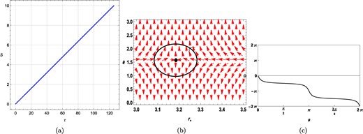
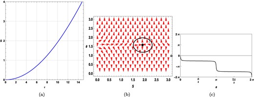
$$\begin{eqnarray} \tau =\frac{4 \pi r_+}{1-3 \kappa r_+^2} . \end{eqnarray}$$

(29)

We plot τ vs r₊ for κ = 0.005 in Fig. 1(a), where we observe one single black hole branch. In Fig. 1(b), a vector plot is shown for the ϕ^r and ϕ^θ components taking τ = 100, where we observe the zero point of the vector field at r₊ = 4.9879. From Fig. 1(c) it is observed that the winding number or the topological charge corresponding to r₊ = 4.9879 is found to be −1, which is represented by the black-colored solid line. Further analysis shows that for all values of κ, the topological charge is always −1.

Fig. 1.

Plots for a static black hole considering model I, where κ = 0.005. (a) τ vs r₊ plot. (b) Plot of the vector field n on a portion of the r₊ − θ plane for τ = 100. The red arrows represent the vector field n. The zero point is located at r₊ = 4.9879. (c) Computation of the winding number for the contour around the zero point, r₊ = 4.9879.

Open in new tab Download slide

2.2. Model II

The second model we have considered is [104]:

$$\begin{eqnarray} \mathrm{ f}(R)=-\frac{\left(R-R_0\right){}^{2 n+1}+R_0^{2 n+1}}{\mathrm{ f}_1 \left\lbrace \left(R-R_0\right){}^{2 n+1}+R_0^{2 n+1}\right\rbrace +\mathrm{ f}_0} \end{eqnarray}$$

(30)

$$\begin{eqnarray} \mathrm{ f}(R)=-\frac{1}{\mathrm{ f}_1}+\frac{\mathrm{ f}_0}{\mathrm{ f}_1 \left(\mathrm{ f}_1 \left\lbrace \left(R-R_0\right){}^{2 n+1}+R_0^{2 n+1}\right\rbrace +\mathrm{ f}_0\right)} , \end{eqnarray}$$

(31)

where

$$\begin{eqnarray} \frac{1}{\mathrm{ f}_1}=\Lambda _i \text{and} \mathrm{ f}_0=\frac{R_0^{2n}}{2}. \end{eqnarray}$$

Here, n = 1, 2, 3.... is a positive integer. R₀ is the current curvature (R₀ ∼ (10⁻³³eV)²) and Λ_i is the effective cosmological constant (Λ_i ∼ 10^20∼38). The details about this model are available in Ref. [104]. For simplicity, we take n = 1 and following the aforementioned procedure, we find out the second-order approximated metric solution of Eq. (12):

$$\begin{eqnarray} ds^2=-\mathrm{ N}(r)dt^2+\mathrm{ M}(r) dr^2+r^2(d\theta ^2+\mathrm{ sin}^2\theta d\phi ^2), \end{eqnarray}$$

where

$$\begin{eqnarray} \mathrm{ N}(r)=1-\frac{2M}{r}+\frac{1}{12} \left(-\sqrt{3} R_0+\frac{6 \sqrt{3} \left(7 \sqrt{3}+12\right) R_0^2}{\Lambda _i}\right) r^2 . \end{eqnarray}$$

(32)

The mass is calculated as:

$$\begin{eqnarray} M=\frac{r_+ \left(12 \Lambda _i-\sqrt{3} r_+^2 R_0 \Lambda _i+72 \sqrt{3} r_+^2 R_0^2+126 r_+^2 R_0^2\right)}{24 \Lambda _i} . \end{eqnarray}$$

(33)

The temperature is given by:

$$\begin{eqnarray} T=\frac{4 \Lambda _i+r_+^2 R_0 \left(18 \left(4 \sqrt{3}+7\right) R_0-\sqrt{3} \Lambda _i\right)}{16 \pi r_+ \Lambda _i} . \end{eqnarray}$$

(34)

And the entropy is calculated as:

$$\begin{eqnarray} S=\pi r_{+}^2 . \end{eqnarray}$$

(35)

From Eqs. (33) and (35), free energy is calculated as:

$$\begin{eqnarray} \mathcal {F}=\mathcal {F}=M-S/\tau =\frac{1}{24} \left(\frac{r_+^3 R_0 \left(18 \left(4 \sqrt{3}+7\right) R_0-\sqrt{3} \Lambda _i\right)}{\Lambda _i}-\frac{24 \pi r_+^2}{\tau }+12 r_+\right) . \end{eqnarray}$$

(36)

The components of the vector ϕ are found to be

$$\begin{eqnarray} \phi ^{r}=\frac{r_+^2 R_0 \left(18 \left(4 \sqrt{3}+7\right) R_0-\sqrt{3} \Lambda _i\right)}{8 \Lambda _i}-\frac{2 \pi r_+}{\tau }+\frac{1}{2} , \end{eqnarray}$$

(37)

$$\begin{eqnarray} \phi ^\Theta =-\cot \Theta ~\csc \Theta . \end{eqnarray}$$

(38)

The expression for τ corresponding to zero points is obtained by setting ϕ^r = 0:

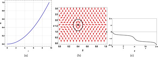
$$\begin{eqnarray} \tau =-\frac{16 \pi r_+ \Lambda _i}{r_+^2 R_0 \left(\sqrt{3} \Lambda _i-18 \left(4 \sqrt{3}+7\right) R_0\right)-4 \Lambda _i} . \end{eqnarray}$$

(39)

Next, we plot τ vs r₊ taking R₀ = (10⁻³³)²eV and Λ_i = 10²⁶ in Fig. 2(a), where we again observe one single black hole branch whose topological charge is −1. The vector plot in Fig. 2(b) and the contourplot in Fig. 4(c) show the same. In fact the topological charge is always −1 for all values of R₀ and Λ_i.

Plots for a static black hole considering model II, where R0 = (10−33)2eV and Λi = 1026. (a) τ vs r+ plot. (b) Plot of the vector field n on a portion of the r+ − θ plane for τ = 40. The red arrows represent the vector field n. The zero point is located at r+ = 3.18309. (c) Computation of the winding number for the contour around the zero point, r+ = 3.18309.

Fig. 2.

Plots for a static black hole considering model II, where R₀ = (10⁻³³)²eV and Λ_i = 10²⁶. (a) τ vs r₊ plot. (b) Plot of the vector field n on a portion of the r₊ − θ plane for τ = 40. The red arrows represent the vector field n. The zero point is located at r₊ = 3.18309. (c) Computation of the winding number for the contour around the zero point, r₊ = 3.18309.

Open in new tab Download slide

2.3. Model III

The next model that will be used in this work is [151,152]:

$$\begin{eqnarray} \mathrm{ f}(R)=R+\Lambda +\frac{R+\Lambda }{R/R_0+2/\alpha }\mathrm{ ln}\left(\frac{R+\Lambda }{R_c}\right) , \end{eqnarray}$$

(40)

where R_c is the integration constant and R₀ = 6α²/d²; d and α are the free parameters of the action. Λ is the cosmological constant.

The metric solution of Eq. (12) is obtained as [151,152]:

$$\begin{eqnarray} \mathrm{ N}(r)=1-\frac{2M}{r}+\beta r -\frac{\Lambda r^2}{3} , \end{eqnarray}$$

(41)

where β = α/d ≥ 0 is a real constant.

From Eq. (41), mass M can be obtained by setting N(r = r₊) = 0, which gives:

$$\begin{eqnarray} M=\frac{r_+ \left(\beta l^2 r_++l^2-r_+^2\right)}{2 l^2} . \end{eqnarray}$$

(42)

We have used |$\Lambda =\frac{3}{l^2}$| [153] in which l is the radius of curvature of the de Sitter space.

The entropy can be obtained by using the radius of the event horizon as:

$$\begin{eqnarray} S=\pi r_+^2 . \end{eqnarray}$$

(43)

Using Eqs. (42) and (43), the free energy |$\mathcal {F}=M-S/\tau$| for a static black hole in this f(R) model is found to be:

$$\begin{eqnarray} \mathcal {F}=\frac{1}{2} r_+ \left(-\frac{r_+^2}{l^2}+r_+ \left(\beta -\frac{2 \pi }{\tau }\right)+1\right) . \end{eqnarray}$$

(44)

The components of the vector ϕ are found to be

$$\begin{eqnarray} \phi ^{r}=\frac{\partial \mathcal {F}}{\partial r_{+}}=-\frac{3 r_+^2}{2 l^2}+r_+ \left(\beta -\frac{2 \pi }{\tau }\right)+\frac{1}{2} , \end{eqnarray}$$

(45)

$$\begin{eqnarray} \phi ^\Theta =-\cot \Theta ~\csc \Theta . \end{eqnarray}$$

(46)

The expression for τ corresponding to zero points is obtained by setting ϕ^r = 0:

$$\begin{eqnarray} \tau =\frac{4 \pi l^2 r_+}{2 \beta l^2 r_++l^2-3 r_+^2} . \end{eqnarray}$$

(47)

It is to be noted that not all values of r₊ and l are allowed for specific values of β. The allowed combinations of values of r₊ and l² for β = 1 are shown in Fig. 3 as the shaded portion with semipositive temperature.

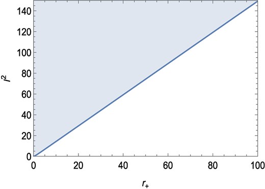
The relation between l2 and r for the positive temperature. Temperature is positive only on the shaded portion. We have taken β = 1.

Fig. 3.

The relation between l² and r for the positive temperature. Temperature is positive only on the shaded portion. We have taken β = 1.

Open in new tab Download slide

From the τ vs r₊ plot in Fig. 4(a), we observe one single black hole branch. The winding number is calculated by keeping β = 1, l² = 100, and τ = 20. For this combination of values, we observe the zero point of the vector field n at r₊ = 46.44048 (Fig. 4(b)). From Fig. 4(c) it is observed that the winding number or the topological charge corresponding to r₊ = 46.44048 (represented by the black-colored solid line) is found to be −1. Further analysis shows that for all sets of values of β, l², the topological charge remains constant, at −1.

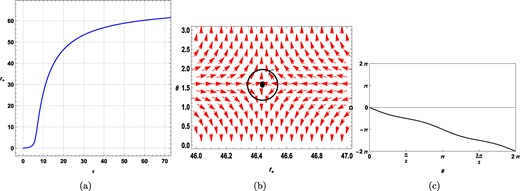
$Plots for a static black hole in model III, at $l^{2}=100$ with β = 1. (a) τ vs r+ plot. (b) Plot of the vector field n on a portion of the r+ − θ plane for τ = 20. The red arrows represent the vector field n. The zero point is located at r+ = 46.44048. (c) Computation of the winding number for the contour around the zero point, r+ = 46.44048.$

Fig. 4.

Plots for a static black hole in model III, at |$l^{2}=100$| with β = 1. (a) τ vs r₊ plot. (b) Plot of the vector field n on a portion of the r₊ − θ plane for τ = 20. The red arrows represent the vector field n. The zero point is located at r₊ = 46.44048. (c) Computation of the winding number for the contour around the zero point, r₊ = 46.44048.

Open in new tab Download slide

3. Charged static black hole in f(R) gravity

The second black hole solution in f(R) gravity that we have chosen to study is a charged static black hole solution originating from the following action [141]:

$$\begin{eqnarray} S=\frac{1}{16 \pi G} \int d^4x \sqrt{-g} \left(R+\mathrm{ f}(R)-F_{\mu \nu } F^{\mu \nu }\right). \end{eqnarray}$$

Varying the action with respect to the metric gives:

$$\begin{eqnarray} R_{\mu \nu }(1+\mathrm{ f}^{\prime }(R)) - \frac{1}{2} \left(R+\mathrm{ f}(R)\right) g_{\mu \nu }+\left(g_{\mu \nu } \nabla ^2-\nabla _\mu \nabla _\nu \right) \mathrm{ f}^{\prime }(R)=2T_{\mu \nu } , \end{eqnarray}$$

where |$\mathrm{ f}^{\prime }(R)=\frac{d\mathrm{ f}(R)}{dR}$| and T_μν is the stress-energy tensor of the electromagnetic field.

The trace of the above equation at R = R₀ results in:

$$\begin{eqnarray} R_0(1+\mathrm{ f}^{\prime }(R_0))-2(R_0+\mathrm{ f}(R_0))=0 , \end{eqnarray}$$

which eventually gives the constant curvature scalar as:

$$\begin{eqnarray} R_0=\frac{2 \mathrm{ f}(R_0)}{\mathrm{ f}^{\prime }(R_0)-1} . \end{eqnarray}$$

Finally, the metric of the spherically symmetric spacetime is obtained as follows:

$$\begin{eqnarray} ds^2=\mathrm{ P}(r)dt^2-\frac{1}{\mathrm{ P}(r)} dr^2-r^2(d\theta ^2+\mathrm{ sin}^2\theta d\phi ^2) , \end{eqnarray}$$

(48)

where

$$\begin{eqnarray} \mathrm{ P}(r)=1-\frac{2 G M}{r}+\frac{Q^2}{\left(1+\mathrm{ f}^{\prime }(R_0)\right) r^2}-\frac{R_0 r^2}{12} . \end{eqnarray}$$

(49)

For details about the metric see Ref. [142].

By putting G = 1 and |$q^2=\frac{Q^2}{\left(1+\mathrm{ f}^{\prime }(R_0)\right)}$| in the above equation:

$$\begin{eqnarray} \mathrm{ P}(r)=1-\frac{2 M}{r}+\frac{q^2}{r^2}-\frac{R_0 r^2}{12} , \end{eqnarray}$$

(50)

where R₀ = 4Λ = |$\frac{12}{l^2}$| is the constant curvature.

3.1. Fixed charge ensemble

For a charged static black hole, from Eq. (50), mass M in the canonical ensemble is obtained as [141]:

$$\begin{eqnarray} M=\frac{\pi ^2 l^2 q^2+\pi l^2 S-S^2}{2 \pi ^{3/2} l^2 \sqrt{S}} . \end{eqnarray}$$

(51)

In the context of the charged static black hole and rotating charged black hole, formulating the vector field component in terms of the horizon radius r₊ is difficult, particularly when working in different ensembles. Consequently, we have performed all calculations in terms of the entropy S. Using Eq. (51), free energy is computed as:

$$\begin{eqnarray} \mathcal {F}=M-S/\tau =\frac{\pi ^2 l^2 q^2 \tau -2 \pi ^{3/2} l^2 S^{3/2}+\pi l^2 S \tau -S^2 \tau }{2 \pi ^{3/2} l^2 \sqrt{S} \tau } . \end{eqnarray}$$

(52)

The components of the vector field ϕ are obtained as:

$$\begin{eqnarray} \left(\phi ^S,\phi ^\Theta \right)=\left(\frac{\partial \mathcal {F}}{\partial S},-\cot \Theta ~\csc \Theta \right), \end{eqnarray}$$

where

$$\begin{eqnarray} \phi ^S=\frac{\pi l^2 \left(-\pi q^2 \tau -4 \sqrt{\pi } S^{3/2}+S \tau \right)-3 S^2 \tau }{4 \pi ^{3/2} l^2 S^{3/2} \tau } \end{eqnarray}$$

(53)

and

$$\begin{eqnarray} \phi ^\Theta =-\cot \Theta ~\csc \Theta . \end{eqnarray}$$

(54)

The zero points of ϕ^r are also obtained as:

$$\begin{eqnarray} \tau =\frac{4 \pi ^{3/2} l^2 S^{3/2}}{-\pi ^2 l^2 q^2+\pi l^2 S-3 S^2} . \end{eqnarray}$$

(55)

For all values of q and l, the static charged black hole has topological charge equal to 0. At, e.g. q = 0.25 and l = 10, we encounter two black hole branches with total topological charge equaling 1 − 1 = 0, as shown in Fig. 5. In Fig. 5(a), τ vs S is plotted in the allowed range of S. For τ = 9, there are two zero points located at S = 0.38868 and S = 1.033022 as shown in Fig. 5(b). From Fig. 5(c), the winding numbers corresponding to S = 0.38868 and S = 1.033022 (represented by the black- and the red-colored solid line, respectively) are found to be −1 and +1, respectively. The total topological charge of the black hole, therefore, is 1 − 1 = 0.

Fig. 5.

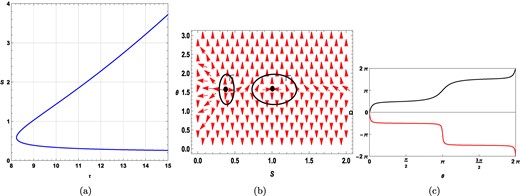
Plots for a static charged black hole in f(R) gravity in the fixed charge ensemble. Here q = 0.25 with l = 10. (a) τ vs S plot. (b) Plot of the vector field n on a portion of the S − θ plane for τ = 40. The red arrows represent the vector field n. The zero points are located at S = 0.38868 and S = 1.033022. (c) Computation of the winding numbers for the contours around the zero points S = 0.38868 and S = 1.033022, shown by the black- and red-colored solid lines, respectively.

Open in new tab Download slide

If we set q = 0, then we encounter one single black hole branch with topological charge −1 as shown in Fig. 6. In Fig. 6(a) τ vs S is plotted in the allowed range of S. For τ = 10, the zero point is located at S = 1.91726 as shown in Fig. 6(b). From Fig. 6(c), the winding number corresponding to S = 1.91726 (represented by the black-colored solid line) is found to be −1. So, when the charge q = 0, the thermodynamic topology of static charged black holes becomes equivalent to that of static black holes as expected.

Fig. 6.

Plots for a static charged black hole in f(R) gravity in the fixed charge ensemble. Here, q = 0 with l = 10. (a) τ vs S plot. (b) Plot of the vector field n on a portion of the S − θ plane for τ = 10. The red arrows represent the vector field n. The zero point is located at S = 1.91726. (c) Computation of the winding number for the contour around the zero point S = 2.5581.

Open in new tab Download slide

3.2. Fixed potential(ϕ) ensemble

In the fixed ϕ ensemble, we define a potential ϕ conjugate to q and keep it fixed. These two parameters are related by

$$\begin{eqnarray} \phi =\frac{\partial M}{\partial q}=\frac{\sqrt{\pi } q}{\sqrt{S}} . \end{eqnarray}$$

The mass in the fixed ϕ canonical ensemble is given by:

$$\begin{eqnarray} \tilde{M}=M-q\phi. \end{eqnarray}$$

We get

$$\begin{eqnarray} \tilde{M}=\frac{\sqrt{S} \left(\pi l^2 \left(1-\phi ^2\right)-S\right)}{2 \pi ^{3/2} l^2} . \end{eqnarray}$$

(56)

Accordingly, the free energy is calculated using:

$$\begin{eqnarray} \tilde{\mathcal {F}}=\tilde{M}-\frac{S}{\tau } \end{eqnarray}$$

(57)

$$\begin{eqnarray} \tilde{\mathcal {F}}=-\frac{\sqrt{S} \left(2 \pi ^{3/2} l^2 \sqrt{S}+\pi l^2 \tau \phi ^2-\pi l^2 \tau +S \tau \right)}{2 \pi ^{3/2} l^2 \tau } . \end{eqnarray}$$

(58)

The components of the vector field are obtained as:

$$\begin{eqnarray} \left(\phi ^S,\phi ^\theta \right)=\left(\frac{\partial \mathcal {F}}{\partial S},-\cot \theta ~\csc \theta \right) , \end{eqnarray}$$

where

$$\begin{eqnarray} \phi ^S=\frac{\pi l^2 \left(-4 \sqrt{\pi } \sqrt{S}-\tau \phi ^2+\tau \right)-3 S \tau }{4 \pi ^{3/2} l^2 \sqrt{S} \tau } \end{eqnarray}$$

(59)

and

$$\begin{eqnarray} \phi ^\theta =-\cot \theta \csc \theta . \end{eqnarray}$$

(60)

Finally, we obtain the expression for τ as:

$$\begin{eqnarray} \tau =\frac{4 \pi ^{3/2} l^2 \sqrt{S}}{-\pi l^2 \phi ^2+\pi l^2-3 S} . \end{eqnarray}$$

(61)

It is seen that for all values of ϕ and l, the static charged black hole in the fixed potential ensemble has a topological charge equal to −1. In Fig. 7(a) a τ vs S plot is shown where ϕ = 0.5 and l = 10. Here, we observe a single black hole branch. For τ = 6, the zero point is located at S = 0.39878. This is also confirmed from the vector plot of n in the S − θ plane as shown in Fig. 7(b). To find out the winding number/topological number associated with this zero point, we perform a contour integration around S = 0.39878, which is shown in Fig. 7(c). The topological charge in this case is equal to −1. We have explicitly verified that the topological charge of any zero point on the black hole branch remains the same and is equal to −1. Strikingly, in the fixed potential ensemble, the topological charge is different from that in the fixed charge ensemble.

Fig. 7.

Plots for a static charged black hole in the fixed potential ensemble at ϕ = 0.5 with l = 10. (a) τ vs S plot. (b) Plot of the vector field n on a portion of the S − θ plane for τ = 6. The red arrows represent the vector field n. The zero point is located at S = 0.39878. (c) Computation of the contour around the zero point τ = 100 and S = 0.39878.

Open in new tab Download slide

4. Rotating charged black hole

In this section, we study the thermodynamic topology of a rotating charged black hole solution in f(R) gravity for four types of ensemble: fixed (q, J), fixed (ϕ, J), fixed (q, Ω), and fixed (ϕ, Ω) ensemble, where q, ϕ, J, and Ω denote the charge, potential, angular momentum, and angular frequency, respectively. The black hole of our interest originates from the following action:

$$\begin{eqnarray} S=\frac{1}{16 \pi }\left(\int d^D x \sqrt{|g|} (R+\mathrm{ f}(R))-\int d^4 x \sqrt{|g|} [F_{\mu \nu }F^{\mu \nu }]\right) , \end{eqnarray}$$

(62)

where the first part represents the gravitational action and the second part represents the 4D Maxwell term. R is the scalar curvature and R + f(R) is a function of the scalar curvature. The field equations in the metric formalism are [143]:

$$\begin{eqnarray} R_{\mu \nu }(1+\mathrm{ f}^{\prime }(R))-\frac{1}{2}(R+\mathrm{ f}(R)) g_{\mu \nu } +(g_{\mu \nu } \nabla ^2 -\nabla _\mu \nabla _\nu )\mathrm{ f}^{\prime }(R)=2 T_{\mu \nu } , \end{eqnarray}$$

(63)

where ∇ is the covariant derivative, R_μν is the Ricci tensor, and T_μν is the stress-energy tensor of the electromagnetic field given by:

$$\begin{eqnarray} T_{\mu \nu }=F_{\mu \rho } F^\rho _\nu -\frac{g_{\mu \nu }}{4} F_{\rho \sigma }F^{\rho \sigma } . \end{eqnarray}$$

The trace of Eq. (63) gives the expression for R = R₀ as:

$$\begin{eqnarray} R_{0}=\frac{2 \mathrm{ f}(R_0)}{\mathrm{ f}^{\prime }(R_0)-1} . \end{eqnarray}$$

(64)

The axisymmetric ansatz, utilizing Boyer–Lindquist-type coordinates (t, r, θ, φ), derived from the Kerr-Newman-AdS black hole solution, as shown in Ref. [143] is:

$$\begin{eqnarray} ds^2=-\frac{\Delta _r}{\rho ^2}\left[ dt-\frac{a \mathrm{ sin}^2\theta d\varphi }{\Xi } \right]^2+\frac{\rho ^2}{\Delta _r} dr^2 +\frac{\rho ^2}{\Delta _\theta } d\theta ^2+\frac{\Delta _\theta \mathrm{ sin}^2 \theta }{\rho ^2}\left[a dt-\frac{r^2+a^2}{\Xi } d\varphi \right]^2 , \end{eqnarray}$$

(65)

where

$$\begin{eqnarray} \Delta _{r}=(r^2+a^2)\left(1+\frac{R_0}{12} r^2 \right)-2mr+\frac{Q^2}{(1+\mathrm{ f}^{\prime }(R_0))}, \end{eqnarray}$$

$$\begin{eqnarray} \Xi =1-\frac{R_0}{12}a^2, \rho ^2=r^2+a^2\mathrm{ cos}^2\theta , \end{eqnarray}$$

$$\begin{eqnarray} \Delta _\theta =1-\frac{R_0}{12}a^2 \mathrm{ cos}^2\theta , \end{eqnarray}$$

in which R₀ = −4Λ, Q is the electric charge, and a is the angular momentum per mass of the black hole. By setting dr = dt = 0 in Eq. (65), we can calculate the area of the 2D horizon, which eventually gives the expression for area as [141]:

$$\begin{eqnarray} S=\frac{\pi (r_+^2+a^2)}{1-\frac{R_0}{12}a^2} , \end{eqnarray}$$

(66)

where r₊ is the radius of the horizon.

The expressions for total mass and the angular momentum are [143]:

$$\begin{eqnarray} M=\frac{m}{\Xi ^2} \end{eqnarray}$$

(67)

and

$$\begin{eqnarray} J=\frac{a m}{\Xi ^2} , \end{eqnarray}$$

(68)

from which the generalized Smarr formula of the rotating charged black hole is obtained as [143]:

$$\begin{eqnarray} M^2=\frac{S}{4 \pi }-\frac{J^2 R_0}{12}+\frac{\pi \left(4 J^2+q^4\right)}{4 S}-\frac{R_0 S \left(q^2-\frac{R_0 S^2}{24 \pi ^2}+\frac{S}{\pi }\right)}{24 \pi }+\frac{q^2}{2} . \end{eqnarray}$$

(69)

4.1. Fixed (q, J) ensemble

In the fixed (q, J) ensemble, we keep q and J as fixed parameters. The mass expression, given by Eq. (69), remains unchanged within this ensemble, and is:

$$\begin{eqnarray} M=\sqrt{\frac{S}{4 \pi }-\frac{J^2 R_0}{12}+\frac{\pi \left(4 J^2+q^4\right)}{4 S}-\frac{R_0 S \left(q^2-\frac{R_0 S^2}{24 \pi ^2}+\frac{S}{\pi }\right)}{24 \pi }+\frac{q^2}{2}} . \end{eqnarray}$$

(70)

The off-shell free energy is calculated to be:

$$\begin{eqnarray} \mathcal {F}=-\frac{24 \pi ^{3/2} S-\tau \sqrt{\frac{-48 \pi ^3 J^2 R S+576 \pi ^4 J^2-24 \pi ^2 q^2 R S^2+288 \pi ^3 q^2 S+144 \pi ^4 q^4+R^2 S^4-24 \pi R S^3+144 \pi ^2 S^2}{S}}}{24 \pi ^{3/2} \tau } . \end{eqnarray}$$

The components of the vector field ϕ are obtained as:

$$\begin{eqnarray} \left(\phi ^S,\phi ^\Theta \right)=\left(\frac{\partial \mathcal {F}}{\partial S},-\cot \Theta ~\csc \Theta \right) \end{eqnarray}$$

$$\begin{eqnarray} \phi ^S=\frac{\partial \mathcal {F}}{\partial S}=\frac{-16 \pi ^{3/2} S^2 \sqrt{\frac{48 \pi ^3 J^2 (12 \pi -R S)+\left(12 \pi ^2 q^2-R S^2+12 \pi S\right)^2}{S}}-48 \pi ^4 \tau \left(4 J^2+q^4\right)-8 \pi ^2 S^2 \tau \left(q^2 R-6\right)+R^2 S^4 \tau -16 \pi R S^3 \tau }{16 \pi ^{3/2} S^2 \tau \sqrt{\frac{48 \pi ^3 J^2 (12 \pi -R S)+\left(12 \pi ^2 q^2-R S^2+12 \pi S\right)^2}{S}}} \end{eqnarray}$$

and

$$\begin{eqnarray} \phi ^\Theta =-\cot \Theta ~\csc \Theta . \end{eqnarray}$$

The expression for τ that corresponds to the zero point of ϕ^S can be obtained by setting ϕ^S = 0:

$$\begin{eqnarray} \tau =\frac{4 \pi ^{3/2} l^4 S^2 \sqrt{\frac{4 \pi ^3 J^2 l^2 \left(\pi l^2+S\right)+\left(\pi l^2 \left(\pi q^2+S\right)+S^2\right)^2}{l^4 S}}}{-4 \pi ^4 J^2 l^4+l^4 \left(\pi ^2 S^2-\pi ^4 q^4\right)+2 \pi l^2 S^2 \left(\pi q^2+2 S\right)+3 S^4} , \end{eqnarray}$$

(71)

where we have substituted |$R_0=-\frac{12}{l^2}$|⁠.

We plot the entropy S against τ for a fixed length scale l = 0.1 while keeping J and q fixed at J = 1.5 and q = 0.05 in Fig. 8. Here we observed a single black hole branch.

Fig. 8.

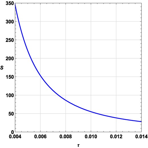
τ vs S plot for a rotating charged black hole in the fixed (q, J) ensemble at q = 0.05, J = 1.5, l = 0.1.

Open in new tab Download slide

In this section, we have adopted another method to calculate the topological charge [74]. The complex function |$\mathcal {R}_{rc}(z)$| defined in Sect. 1 is given by:

$$\begin{eqnarray} \mathcal {R}_{rc}(z)=-\frac{-4 \pi ^4 J^2 l^4+2 \pi ^2 l^2 q^2 z^2-\pi ^4 l^4 q^4+\pi ^2 l^4 z^2+4 \pi l^2 z^3+3 z^4}{4 \pi ^{3/2} l^4 z^2 \sqrt{\frac{4 \pi ^3 J^2 l^2 \left(\pi l^2+z\right)+\left(\pi l^2 \left(\pi q^2+z\right)+z^2\right)^2}{l^4 z}}+4 \pi ^4 J^2 l^4 \tau +\pi ^4 l^4 q^4 \tau -2 \pi ^2 l^2 q^2 \tau z^2-\pi ^2 l^4 \tau z^2-4 \pi l^2 \tau z^3-3 \tau z^4}.\\ \end{eqnarray}$$

(72)

Considering the denominator of the equation as a polynomial function |$\mathcal {A}(z)$| we can calculate the poles of |$\mathcal {R}_{rc}(z)$|⁠:

$$\begin{eqnarray} \mathcal {A}(z)=l^4 \left(4 \pi ^{3/2} z^2 \sqrt{\frac{4 \pi ^3 J^2 l^2 \left(\pi l^2+z\right)+\left(\pi l^2 \left(\pi q^2+z\right)+z^2\right)^2}{l^4 z}}+\pi ^4 \tau \left(4 J^2+q^4\right)-\pi ^2 \tau z^2\right)-2 \pi l^2 \tau z^2 \left(\pi q^2+2 z\right)-3 \tau z^4 .\\ \end{eqnarray}$$

(73)

To get the winding number, we put l = 0.1, J = 1.5, and q = 0.05 in Eq. (73). It is seen from Fig. 9 that, for τ = 0.008, the pole is at z = 86.108. The winding number can be calculated by finding the sign of the residue of Eq. (72) around the pole z = 86.108. We find a positively valued residue in this case. Hence, the winding number or the total topological charge is 1. It is found that if the value of l is decreased below l = 0.1, no branch or topological charge remains the same.

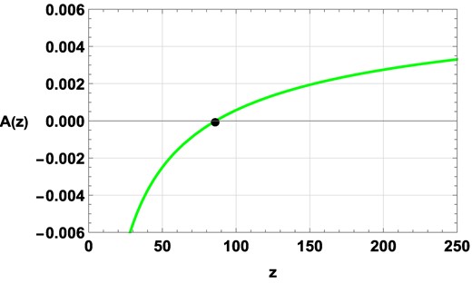
$Plot for polynomial function $\mathcal {A}(z)$ for τ = 0.008.$

Fig. 9.

Plot for polynomial function |$\mathcal {A}(z)$| for τ = 0.008.

Open in new tab Download slide

In Fig. 10, we have plotted S against τ when the length scale is increased to l = 10 while keeping q = 0.05 and J = 1.5 fixed. Here we observe three black hole branches: a small, an intermediate, and a large black hole branch. We also see a generation point at τ = 36.5182, S = 97.4031 and an annihilation point at τ = 33.8834, S = 28.8408, which are shown as black dots. To calculate the winding numbers, we put l = 10, J = 1.5, and q = 0.05 in Eq. (73).

Fig. 10.

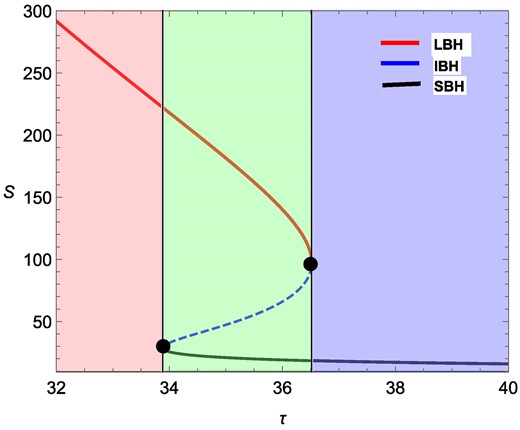
Plots for zero points of ϕ^r in the τ − S plane for a rotating charged black hole in the fixed (q, J) ensemble at l = 10, J = 1.5, and q = 0.05. Two lines are drawn at τ = 36.5182 and τ = 33.8834, which correspond to the annihilation point and the generation point, respectively. The solid red portion represents a large black hole (LBH) branch, the blue dashed portion represents an intermediate black hole (IBH) branch, and the solid black portion represents a small black hole (SBH) branch.

Open in new tab Download slide

The plot for the corresponding |$\mathcal {A}(z)$| is shown in Fig. 11. This clearly shows that for τ < 33.8834, there is only one pole, for 33.8834 < τ < 36.5182 there are three poles, and for τ > 36.5182 there is one pole. For the large black hole branch, taking τ = 33, the pole is at z = 254.214. Around the pole z = 254.214, the winding number is found to be w = +1. For the intermediate black hole branch, taking τ = 35, the poles are at z₁ = 21.0537, z₂ = 47.3137, and z₃ = 181.45. According to the sign of the residue around these three poles, the winding numbers are found to be w₁ = +1, w₂ = −1, and w₃ = +1, respectively. Hence the topological charge is:

$$\begin{eqnarray} W=w_1+w_2+w_3=1-1+1=1 . \end{eqnarray}$$

Similarly, for a small black hole branch, taking τ = 33, the pole is at z = 17.9982 and according to the sign of the residue around the pole, the winding number is found to be +1. We have checked that even if the value of l is increased further (i.e. beyond l = 10), the number of branches and topological charge remain the same.

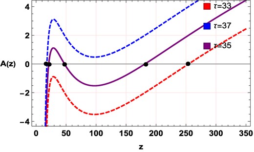
$Plot for polynomial function $\mathcal {A}(z)$ for τ = 33, τ = 35, and τ = 37.$

Fig. 11.

Plot for polynomial function |$\mathcal {A}(z)$| for τ = 33, τ = 35, and τ = 37.

Open in new tab Download slide

We repeat the analysis for different values of J and q, keeping l constant. We observe no effect on the topological charge. The same is illustrated in Fig. 12. In Fig. 12(a), Fig. 12(b), and Fig. 12(c) we show the effect of change in charge q when J and l are kept fixed at J = 1.5 and l = 10. In Fig. 12(a) the charge is changed to a significantly small value q = 0.0001. Here, we observe three black hole branches and the topological charge is found to be 1. In Fig. 12(b) where we set q = 1.3, again we find the number of black hole branches equal to three and topological charge to be 1. When the value of the charge is changed to q = 2 in Fig. 12(c), the number of branches becomes one but the topological charge remains 1.

Fig. 12.

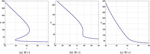
τ vs S plots for a rotating charged black hole in the fixed (q, J) ensemble when charge q is varied for a fixed length l = 10 while keeping J fixed at J = 1.5. (a) τ vs S plot at q = 0.0001, J = 1.5, l = 10; (b) τ vs S plot at q = 1.3, J = 1.5, l = 10; (c) the same at q = 2, J = 1.5, l = 10. W denotes the total topological charge.

Open in new tab Download slide

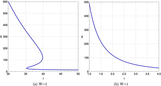
For fixed values of l = 10 and q = 0.05 the effect of variation in J on the thermodynamic topology is demonstrated in Fig. 13(a) and Fig. 13(b). For J = 1, three black hole branches are observed with the sum of the corresponding winding number equal to 1, as shown in Fig. 13(a). In Fig. 13(b) we set J = 7 and find a single black hole branch with topological charge equal to 1. We have explicitly verified that even for other values of J, the topological charge remains the same.

Fig. 13.

τ vs S plots for a rotating charged black hole in the fixed (q, J) ensemble when J is varied for a fixed length l = 10 while keeping the charge fixed at q = 0.05. (a) τ vs S plot at q = 0.05, J = 1, l = 10; (b) the same at q = 0.05, J = 7, l = 10. W denotes the corresponding topological charge.

Open in new tab Download slide

From our analysis, we conclude that the topological charge of the rotating charged black hole in the fixed (q, J) ensemble is equal to +1 and is unaffected by variation in the thermodynamic parameters l, q, J.

4.2. Fixed (ϕ,J) ensemble

In the fixed (ϕ, J) ensemble, the potential ϕ and angular momentum J are kept fixed. The potential ϕ is given by:

$$\begin{eqnarray} \phi =\frac{\partial M}{\partial q}=\frac{\sqrt{\pi } q \left(12 \pi ^2 q^2-R S^2+12 \pi S\right)}{S \sqrt{\frac{48 \pi ^3 J^2 (12 \pi -R S)+\left(12 \pi ^2 q^2-R S^2+12 \pi S\right)^2}{S}}} . \end{eqnarray}$$

(74)

Solving Eq. (74), we get an expression for q and find out the new mass (M_ϕ) in this ensemble as follows:

$$\begin{eqnarray} M_{\phi }=M-q \phi . \end{eqnarray}$$

(75)

The off-shell free energy is computed using:

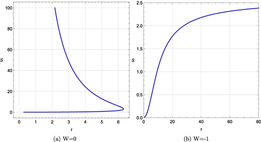
$$\begin{eqnarray} \mathcal {F}=M_{\phi }-S/\tau. \end{eqnarray}$$

Following the same procedure as shown in the previous subsection, we calculate the expressions for ϕ^S and τ. We plot the τ vs S curve for two different values of scalar curvature R as shown in Fig. 14. Here, J and ϕ are kept constant with J = 1.5 and ϕ = 0.05. In Fig. 14(a), we set R = −0.1 and find three black hole branches with topological charge equaling 1. In Fig. 14(b) for R = −4, we observed a single black hole branch with topological charge still equaling 1. We have checked that for the other values of R, the topological charge remains equal to 1.

Fig. 14.

τ vs S plots for a rotating charged black hole in the fixed (ϕ, J) ensemble when scalar curvature R is varied while keeping J and ϕ constant at J = 1.5, ϕ = 0.05. (a) τ vs S plot at ϕ = 0.05, J = 1.5, R = −0.1; (b) τ vs S plot at ϕ = 0.05, J = 1.5, R = −4. W denotes the respective topological charge.

Open in new tab Download slide

Next, we study the influence of changing J on the topological charge with R and ϕ kept fixed at R = −0.1 and ϕ = 0.05, as shown in Fig. 15. In Fig. 15(a) we observe three black hole branches leading to a topological charge of 1. In Fig. 15(b), we again encounter three branches and a topological charge equal to 1, for J = 7. In Fig. 15(c), with J = 10 we get one black hole branch with a topological charge equaling 1. We have explicitly verified that for other values of J the topological charge remains the same.

Fig. 15.

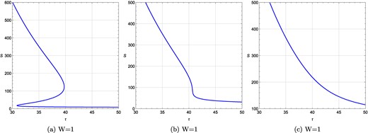
τ vs S plots for a rotating charged black hole in the fixed (ϕ, J) ensemble when J is varied keeping R = −0.1, ϕ = 0.05 fixed. (a) τ vs S plot at ϕ = 0.05, J = 1, R = −0.1; (b) τ vs S plot at ϕ = 0.05, J = 7, R = −0.1; (c) the same at ϕ = 0.05, J = 10, R = −0.1. W denotes the topological charge.

Open in new tab Download slide

Finally, we analyzed the effect of ϕ on the topological charge with fixed values of R and J. τ vs S plots for J = 1.5 and R = −0.1 are shown in Fig. 16(a) and Fig. 16(b) by setting ϕ = 0.005 and ϕ = 3, respectively. Whereas in Fig. 16(a) we find a single black hole branch, in Fig. 16(b) we see three branches. In both cases, the topological charge is found to be 1. The same is found to be true for other values of ϕ with J and R kept fixed.

Fig. 16.

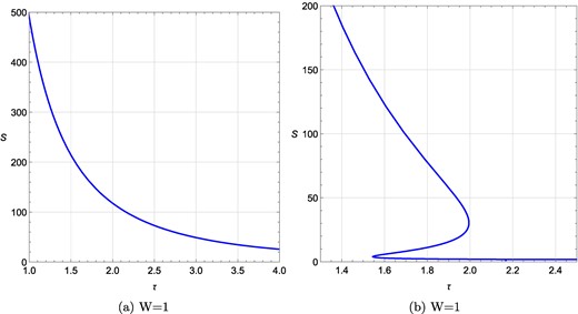
τ vs S plots for a rotating charged black hole in the fixed (ϕ, J) ensemble when ϕ is varied keeping R = −4, J = 1.5 fixed. (a) τ vs S plot at ϕ = 0.005, J = 1.5, R = −4; (b) τ vs S plot at ϕ = 3, J = 1.5, R = −4. W denotes the topological charge.

Open in new tab Download slide

Therefore, we infer that the topological charge of the rotating charged black hole under consideration in the fixed (ϕ, J) ensemble is equal to 1 irrespective of the values of the thermodynamic parameters ϕ, J, and R.

4.3. Fixed (Ω, q) ensemble

Next, we work in the fixed (Ω, q) ensemble where the angular frequency Ω and charge q are kept fixed. We begin with solving the following equation for the angular momentum J:

$$\begin{eqnarray} \Omega =\frac{\partial M}{\partial J}=-\frac{2 \pi ^{3/2} J (R S-12 \pi )}{S \sqrt{\frac{48 \pi ^3 J^2 (12 \pi -R S)+\left(12 \pi ^2 q^2-R S^2+12 \pi S\right)^2}{S}}} . \end{eqnarray}$$

(76)

From Eq. (76) we obtain the expressions for J as follows:

$$\begin{eqnarray} J=\frac{\sqrt{S} \Omega \left(12 \pi ^2 q^2-R S^2+12 \pi S\right)}{2 \pi ^{3/2} \sqrt{(12 \pi -R S) \left(12 \pi -S \left(R+12 \Omega ^2\right)\right)}} . \end{eqnarray}$$

(77)

The new mass (M_Ω) in this ensemble is obtained as:

$$\begin{eqnarray} M_{\Omega }=M-J \Omega , \end{eqnarray}$$

(78)

$$\begin{eqnarray} M_\Omega =\frac{\sqrt{(12 \pi -R S) \left(12 \pi -S \left(R+12 \Omega ^2\right)\right)} \sqrt{\frac{(12 \pi -R S) \left(12 \pi ^2 q^2-R S^2+12 \pi S\right)^2}{S \left(-R S-12 S \Omega ^2+12 \pi \right)}}-144 \pi ^2 q^2 \sqrt{S} \Omega ^2+12 R S^{5/2} \Omega ^2-144 \pi S^{3/2} \Omega ^2}{24 \pi ^{3/2} \sqrt{(12 \pi -R S) \left(12 \pi -S \left(R+12 \Omega ^2\right)\right)}} .\\ \end{eqnarray}$$

(79)

Accordingly, the off-shell free energy is computed using:

$$\begin{eqnarray} \mathcal {F}=M_{\Omega }-S/\tau . \end{eqnarray}$$

Repeating the procedure alluded to in the previous section, we obtained the expression for ϕ^S and τ.

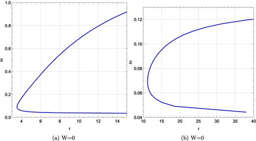
First, we analyzed the dependence of topological charge on the scalar curvature R keeping Ω and q fixed. In Fig. 17(a) and 17(b), τ vs S plots are shown with Ω = 0.1, q = 0.1 kept fixed and R = −0.01 and R = −4, respectively. In Fig. 17(a) two black hole branches and topological charge 0 are observed. In Fig. 17(b), we have three black hole branches totaling a topological charge of 1. Therefore, depending on the value of the scalar curvature, the topological charge is found to be either 0 or 1. For other values of R, we arrived at the same topological charge (0 or 1).

Fig. 17.

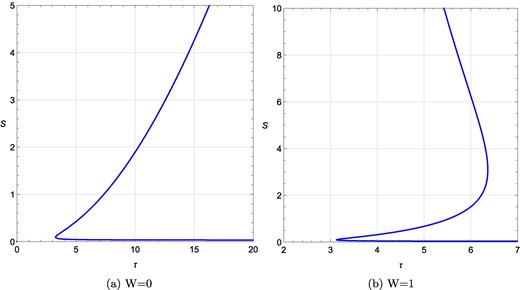
τ vs S plots for a rotating charged black hole in the fixed (Ω, q) ensemble for different values of R. (a) τ vs S plot at Ω = 0.1, q = 0.1, R = −0.01; (b) the same at Ω = 0.1, q = 0.1, R = −4. W denotes the topological charge.

Open in new tab Download slide

Now we want to understand the impact of change in charge q on the topological charge. In Fig. 18(a) and Fig. 18(b), we set Ω = 0.1, R = −4, and q = 0.09 and 1, respectively. In Fig. 18(a) we find three black hole branches, in Fig. 18(b) we find a single black hole branch. The topological charge in both cases equals 1.

Fig. 18.

τ vs S plots for a rotating charged black hole in the fixed (Ω, q) ensemble for different q values when R = −4 and Ω = 0.1 are kept fixed. (a) τ vs S plot at Ω = 0.1, q = 0.09, R = −4; (b) τ vs S plot at Ω = 0.1, q = 1, R = −4. W denotes the topological charge.

Open in new tab Download slide

In Fig. 19(a) and 19(b) we repeat the same analysis with Ω = 0.1, R = −0.01, and q = 0.09 and q = 1, respectively. The number of branches and the topological charge in both cases are found to be identical (two black hole branches and topological charge 0). Hence it is found that the topological charge does not change with the charge q, although the number of black hole branches may vary with a variation in q.

Fig. 19.

τ vs S plots for a rotating charged black hole in the fixed (Ω, q) ensemble for different q values at R = −0.01 and Ω = 0.1. (a) τ vs S plot at q = 0.09; (b) τ vs S plot at q = 1. The topological charge for all cases is 1. W denotes the topological charge.

Open in new tab Download slide

Finally, we examine the role of Ω in determining the topological charge. For that, we keep R and q fixed at R = −0.01 and q = 0.1 in Fig. 20(a) and Fig. 20(b). In Fig. 20(a) and 20(b) we set Ω = 1 and Ω = 3, respectively. As seen from the figure, the topological charge remains unaffected by the variation in Ω and is equal to 0. In conclusion, our results indicate that the topological charge of the rotating charged black hole in the fixed (Ω, q) ensemble is either 0 or 1 depending on the values of R. The other thermodynamic parameters Ω and q do not have any impact on the topological charge.

Fig. 20.

τ vs S plots for a rotating charged black hole in the fixed (Ω, q) ensemble for different Ω values at R = −0.01 and q = 0.1. (a) τ vs S plot at Ω = 1; (b) τ vs S plot at Ω = 3. The topological charge for all cases is 0.

Open in new tab Download slide

4.4. Fixed (Ω, Φ) ensemble

The last ensemble in which we conduct our analysis is the fixed (Ω, ϕ) ensemble. In this ensemble Ω and ϕ are kept fixed. First, we substitute J from Eq. (77) in the expression for mass in Eq. (69) as follows:

$$\begin{eqnarray} M=\sqrt{\frac{(R S-12 \pi ) \left(12 \pi ^2 q^2-R S^2+12 \pi S\right)^2}{576 \pi ^3 S \left(S \left(R+12 \Omega ^2\right)-12 \pi \right)}} . \end{eqnarray}$$

(80)

Now Eq. (80) becomes independent of variable J. From Eq. (80), we compute ϕ as:

$$\begin{eqnarray} \phi =\frac{dM_J}{dq}=\frac{\sqrt{\pi } q \sqrt{\frac{(R S-12 \pi ) \left(12 \pi ^2 q^2-R S^2+12 \pi S\right)^2}{S \left(S \left(R+12 \Omega ^2\right)-12 \pi \right)}}}{12 \pi ^2 q^2-R S^2+12 \pi S} . \end{eqnarray}$$

(81)

Accordingly, q is given by Eq. (81) as:

$$\begin{eqnarray} q=\frac{\sqrt{S} \phi \sqrt{R S+12 S \Omega ^2-12 \pi }}{\sqrt{\pi } \sqrt{R S-12 \pi }} . \end{eqnarray}$$

The new expression for angular momentum (J) is given by:

$$\begin{eqnarray} J=\frac{S^{3/2} \Omega \left(R^2 S^2-12 \pi R S \phi ^2-24 \pi R S-144 \pi S \Omega ^2 \phi ^2+144 \pi ^2 \phi ^2+144 \pi ^2\right)}{2 \pi ^{3/2} (12 \pi -R S) \sqrt{(12 \pi -R S) \left(-R S-12 S \Omega ^2+12 \pi \right)}} . \end{eqnarray}$$

Finally, the modified mass in the fixed (Ω, Φ) ensemble is written as:

$$\begin{eqnarray} \tilde{M}=M-q \phi -J \Omega \end{eqnarray}$$

(82)

$$\begin{multline} \tilde{M}= \frac{\sqrt{\frac{S \left(R^2 S^2-12 \pi S \left(R \left(\phi ^2+2\right)+12 \Omega ^2 \phi ^2\right)+144 \pi ^2 \left(\phi ^2+1\right)\right)^2}{(12 \pi -R S) \left(12 \pi -S \left(R+12 \Omega ^2\right)\right)}}}{24 \pi ^{3/2}} - \frac{S^{3/2} \Omega ^2 \left(\frac{12 \pi \phi ^2 \left(S \left(R+12 \Omega ^2\right)-12 \pi \right)}{R S-12 \pi }-R S+12 \pi \right)}{2 \pi ^{3/2} \sqrt{(12 \pi -R S) \left(12 \pi -S \left(R+12 \Omega ^2\right)\right)}} \\ - \frac{\sqrt{S} \phi ^2 \sqrt{S \left(R+12 \Omega ^2\right)-12 \pi }}{\sqrt{\pi } \sqrt{R S-12 \pi }} . \end{multline}$$

(83)

Using Eq. (83), |$\mathcal {F}$|⁠, ϕ^S, and τ are constructed following standard procedure.

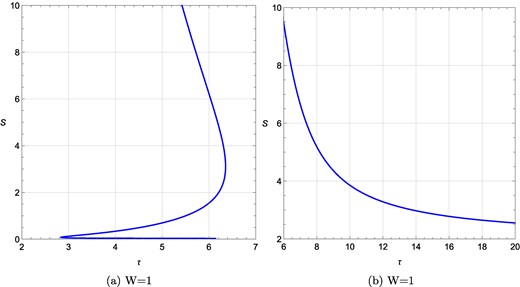
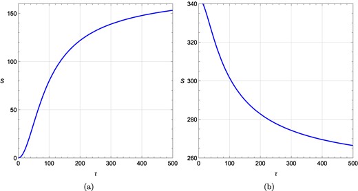
We plot the τ vs S curve for different values of R as shown in Fig. 21 keeping Ω = 0.1, ϕ = 0.1 constant. In Fig. 21(a), with Ω = 0.1, ϕ = 0.1, and R = −0.01, one black hole branch with topological charge W = −1 is observed. With the same values of Ω and ϕ but for different values of R at R = −4, in Fig. 21(b) two black hole branches and topological charge 0 are found.

Fig. 21.

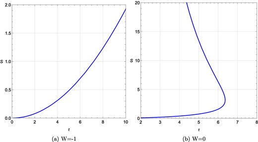
τ vs S plots for a rotating charged black hole in the fixed (Ω, ϕ) ensemble for different values of R. (a) τ vs S plot at Ω = 0.1, ϕ = 0.1, R = −0.01; (b) τ vs S plot at Ω = 0.1, ϕ = 0.1, R = −4. W denotes the topological charge.

Open in new tab Download slide

Next, in Fig. 22(a) and Fig. 22(b), we fix ϕ = 0.1, R = −4 and vary Ω. In Fig. 22(a) setting Ω = 0.001 we get two black hole branches and topological charge W = 0. In Fig. 22(b) with Ω = 1 a single black hole branch with topological charge W = −1 is observed.

Fig. 22.

τ vs S plots for a rotating charged black hole in the fixed (Ω, ϕ) ensemble for different Ω values when R = −4 and ϕ = 0.1 are kept fixed. (a) τ vs S plot at Ω = 0.001, ϕ = 0.1, R = −4; (b) τ vs S plot at Ω = 1, ϕ = 0.1, R = −4. W denotes the total topological charge.

Open in new tab Download slide

Finally, we probe the thermodynamic topology with reference to a variation in the potential ϕ in Fig. 23(a) and 23(b), where we set Ω = 0.1, R = −4, and ϕ = 0.001 and ϕ = 2, respectively. Whereas in the first case, we find two black hole branches and winding number W = 0, in the latter case a single black hole branch with topological charge 1 is found.

Fig. 23.

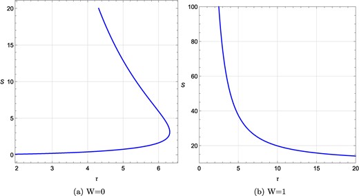
τ vs S plots for a rotating charged black hole in the fixed (Ω, ϕ) ensemble for different ϕ values when R = −4 and Ω = 0.1 are kept fixed. (a) τ vs S plot at ϕ = 0.001, Ω = 0.1, R = −4; (b) τ vs S plot at ϕ = 1, Ω = 0.1, R = −4. W denotes the topological charge.

Open in new tab Download slide

We continue our study at a different value of R equal to −0.01 in Fig. 24(a) and Fig. 24(b). In Fig. 24(a), Ω = 0.1 and ϕ = 0.001. In Fig. 24(b), Ω is again fixed at 0.1 but ϕ is changed to ϕ = 2. For ϕ = 0.001 a single black hole branch with topological charge W = −1 is seen. For ϕ = 2 we again encounter a single black hole branch, but this time with a topological charge of +1.

To summarize, the topological charge for the rotating charged black hole in the fixed (Ω, ϕ) ensemble is −1, 0, or +1 depending on all the thermodynamic parameters R, Ω, and ϕ.

Fig. 24.

τ vs S plots for a rotating charged black hole in the fixed (Ω, ϕ) ensemble for different ϕ values when R = −0.01 and Ω = 0.1 are kept fixed. (a) τ vs S plot at ϕ = 0.001, Ω = 0.1, R = −0.01; (b) τ vs S plot at ϕ = 2, Ω = 0.1, R = −0.01. W denotes the topological charge.

Open in new tab Download slide

5. Conclusion

In this study, we have analyzed the thermodynamic topology of a static black hole, a charged static black hole, and a charged rotating black hole within the framework of f(R) gravity. We have considered two distinct ensembles for charged static black holes: the fixed charge (q) ensemble and the fixed potential (ϕ) ensemble. For charged rotating black holes, we have explored four different ensembles: fixed (q, J), fixed (ϕ, J), fixed (q, Ω), and fixed (ϕ, Ω) ensembles. Considering these black holes as topological defects at thermodynamic spaces, we have computed the associated winding numbers or the topological charges to study the local and global topologies of these black holes.

It has been observed that for the static black hole, the topological charge remains constant at −1, irrespective of the three models we have considered and the respective thermodynamic parameters of the model.

In the case of the static charged black hole in a fixed charge ensemble, the topological charge is computed to be 0 and it does not change with variations in the charge q and the curvature radius l. However, in the fixed potential ensemble, for the charged static black hole, the topological charge is found to be −1. In this scenario as well, the topological charge remains unaffected by variations in the potential ϕ and the curvature radius l.

In the case of the rotating charged black hole, we have considered four ensembles and the results obtained in those ensembles can be summarized as follows. For the fixed (q, J) ensemble, the topological charge is found to be 1 and it does not vary with charge q, angular momentum J, and curvature radius l. However, for different length scales, the number of branches in the τ vs S plot changes with variation of q, J, and l. Although it does not result in a change of the topological charge.

In the case of the fixed (ϕ, J) ensemble, the topological charge is found to be 1 and it does not depend upon the values of potential ϕ, J, and scalar curvature R. Again the number of branches in the τ vs S plot varies with changes in ϕ, J, and R values while keeping the topological charge unchanged.

In the case of the fixed (q, Ω) ensemble, the topological charge is 1 or 0 depending on the value of the scalar curvature R. Although the number of branches of the τ vs S plot changes with variation of q and Ω values for a fixed R, the topological charge remains unaltered.

Finally, in the fixed (Ω, ϕ) ensemble, the topological charge is −1, 0, or 1 depending on the values of R, Ω, and ϕ. The results for the charged rotating black hole case are summarized in Table 1.

Open in new tab

Fixed (q, J) ensemble	q	J	l	Number of branches in τ vs S plot	Topological charge
	0.05	1.5	0.1	1	1
	0.05	7	0.1	1	1
	0.001	1.5	0.1	1	1
	2	1.5	0.1	1	1
	0.05	1.5	10	3	1
	0.05	7	10	1	1
	0.001	1.5	10	3	1
	2	1.5	10	1	1
Fixed (ϕ, J) ensemble	ϕ	J	R
	0.05	1.5	−0.1	3	1
	0.05	10	−0.1	1	1
	0.005	1.5	−0.1	3	1
	3	1.5	−0.1	3	1
	0.05	1.5	−4	1	1
	0.05	3	−4	1	1
	0.005	1.5	−4	1	1
	3	1.5	−4	3	1
Fixed (q, Ω) ensemble	q	Ω	R
	0.1	0.1	−0.01	2	0
	0.1	0.01	−0.01	2	0
	0.1	3	−0.01	2	0
	0.09	0.1	−0.01	2	0
	1	0.1	−0.01	2	0
	0.1	0.1	−4	3	1
	0.1	0.001	−4	3	1
	0.1	1	−4	3	1
	0.09	0.1	−4	3	1
	1	0.1	−4	1	1
Fixed (Ω, ϕ) ensemble	ϕ	Ω	R
	0.1	0.1	−0.01	1	−1
	0.1	0.001	−0.01	1	−1
	0.1	1	−0.01	1	−1
	0.001	0.1	−0.01	1	−1
	2	0.1	−0.01	1	1
	0.1	0.1	−4	2	0
	0.1	0.001	−4	2	0
	0.1	1	−4	1	−1
	0.001	0.1	−4	2	0
	1	0.1	−4	1	1

Fixed (q, J) ensemble	q	J	l	Number of branches in τ vs S plot	Topological charge
	0.05	1.5	0.1	1	1
	0.05	7	0.1	1	1
	0.001	1.5	0.1	1	1
	2	1.5	0.1	1	1
	0.05	1.5	10	3	1
	0.05	7	10	1	1
	0.001	1.5	10	3	1
	2	1.5	10	1	1
Fixed (ϕ, J) ensemble	ϕ	J	R
	0.05	1.5	−0.1	3	1
	0.05	10	−0.1	1	1
	0.005	1.5	−0.1	3	1
	3	1.5	−0.1	3	1
	0.05	1.5	−4	1	1
	0.05	3	−4	1	1
	0.005	1.5	−4	1	1
	3	1.5	−4	3	1
Fixed (q, Ω) ensemble	q	Ω	R
	0.1	0.1	−0.01	2	0
	0.1	0.01	−0.01	2	0
	0.1	3	−0.01	2	0
	0.09	0.1	−0.01	2	0
	1	0.1	−0.01	2	0
	0.1	0.1	−4	3	1
	0.1	0.001	−4	3	1
	0.1	1	−4	3	1
	0.09	0.1	−4	3	1
	1	0.1	−4	1	1
Fixed (Ω, ϕ) ensemble	ϕ	Ω	R
	0.1	0.1	−0.01	1	−1
	0.1	0.001	−0.01	1	−1
	0.1	1	−0.01	1	−1
	0.001	0.1	−0.01	1	−1
	2	0.1	−0.01	1	1
	0.1	0.1	−4	2	0
	0.1	0.001	−4	2	0
	0.1	1	−4	1	−1
	0.001	0.1	−4	2	0
	1	0.1	−4	1	1

Open in new tab

Fixed (q, J) ensemble	q	J	l	Number of branches in τ vs S plot	Topological charge
	0.05	1.5	0.1	1	1
	0.05	7	0.1	1	1
	0.001	1.5	0.1	1	1
	2	1.5	0.1	1	1
	0.05	1.5	10	3	1
	0.05	7	10	1	1
	0.001	1.5	10	3	1
	2	1.5	10	1	1
Fixed (ϕ, J) ensemble	ϕ	J	R
	0.05	1.5	−0.1	3	1
	0.05	10	−0.1	1	1
	0.005	1.5	−0.1	3	1
	3	1.5	−0.1	3	1
	0.05	1.5	−4	1	1
	0.05	3	−4	1	1
	0.005	1.5	−4	1	1
	3	1.5	−4	3	1
Fixed (q, Ω) ensemble	q	Ω	R
	0.1	0.1	−0.01	2	0
	0.1	0.01	−0.01	2	0
	0.1	3	−0.01	2	0
	0.09	0.1	−0.01	2	0
	1	0.1	−0.01	2	0
	0.1	0.1	−4	3	1
	0.1	0.001	−4	3	1
	0.1	1	−4	3	1
	0.09	0.1	−4	3	1
	1	0.1	−4	1	1
Fixed (Ω, ϕ) ensemble	ϕ	Ω	R
	0.1	0.1	−0.01	1	−1
	0.1	0.001	−0.01	1	−1
	0.1	1	−0.01	1	−1
	0.001	0.1	−0.01	1	−1
	2	0.1	−0.01	1	1
	0.1	0.1	−4	2	0
	0.1	0.001	−4	2	0
	0.1	1	−4	1	−1
	0.001	0.1	−4	2	0
	1	0.1	−4	1	1

Fixed (q, J) ensemble	q	J	l	Number of branches in τ vs S plot	Topological charge
	0.05	1.5	0.1	1	1
	0.05	7	0.1	1	1
	0.001	1.5	0.1	1	1
	2	1.5	0.1	1	1
	0.05	1.5	10	3	1
	0.05	7	10	1	1
	0.001	1.5	10	3	1
	2	1.5	10	1	1
Fixed (ϕ, J) ensemble	ϕ	J	R
	0.05	1.5	−0.1	3	1
	0.05	10	−0.1	1	1
	0.005	1.5	−0.1	3	1
	3	1.5	−0.1	3	1
	0.05	1.5	−4	1	1
	0.05	3	−4	1	1
	0.005	1.5	−4	1	1
	3	1.5	−4	3	1
Fixed (q, Ω) ensemble	q	Ω	R
	0.1	0.1	−0.01	2	0
	0.1	0.01	−0.01	2	0
	0.1	3	−0.01	2	0
	0.09	0.1	−0.01	2	0
	1	0.1	−0.01	2	0
	0.1	0.1	−4	3	1
	0.1	0.001	−4	3	1
	0.1	1	−4	3	1
	0.09	0.1	−4	3	1
	1	0.1	−4	1	1
Fixed (Ω, ϕ) ensemble	ϕ	Ω	R
	0.1	0.1	−0.01	1	−1
	0.1	0.001	−0.01	1	−1
	0.1	1	−0.01	1	−1
	0.001	0.1	−0.01	1	−1
	2	0.1	−0.01	1	1
	0.1	0.1	−4	2	0
	0.1	0.001	−4	2	0
	0.1	1	−4	1	−1
	0.001	0.1	−4	2	0
	1	0.1	−4	1	1

Therefore, we conclude that the thermodynamic topologies of the charged static black hole and charged rotating black hole are influenced by the choice of ensemble. In addition, the thermodynamic topology of the charged rotating black hole also depends on the thermodynamic parameters.

It will be interesting to study the thermodynamic topology of various black hole systems in other modified theories of gravity. We plan to do so in our future work.

Funding

Open Access funding: SCOAP³.

References

[1]

S. W.

Hawking

Phys. Rev. Lett.

1344

(

1971

Month:	Total Views:
March 2024	66
April 2024	131
May 2024	96
June 2024	41
July 2024	20
August 2024	40
September 2024	37
October 2024	42
November 2024	45
December 2024	47
January 2025	42
February 2025	34
March 2025	37
April 2025	31
May 2025	4

Article Contents

Thermodynamic Topology of Black Holes in f(R) Gravity

Abstract

1. Introduction

2. Static black hole in f(R) gravity

2.1. Model I

2.2. Model II

2.3. Model III

3. Charged static black hole in f(R) gravity

3.1. Fixed charge ensemble

3.2. Fixed potential(ϕ) ensemble

4. Rotating charged black hole

4.1. Fixed (q, J) ensemble

4.2. Fixed (ϕ,J) ensemble

4.3. Fixed (Ω, q) ensemble

4.4. Fixed (Ω, Φ) ensemble

5. Conclusion

Funding

References

Citations

Views

Altmetric

Email alerts

Astrophysics Data System

Citing articles via

Latest

Most Read

Most Cited

This Feature Is Available To Subscribers Only