Abstract
This paper studies the exponential of the sum of two non-commuting operators as an infinite product of exponential operators involving repeated commutators of increasing order. It will be shown how to determine the two coefficients in front of the nested commutators in the Zassenhaus formula. The knowledge of one coefficient is enough to generate closed formulas that have several applications in solving problems ranging from linear differential equations and quantum mechanics to non-linear differential equations.
1. Introduction
A crucial problem of mathematical physics is the development of the exponential of the sum of two non-commuting operators. Deeply related to this problem are the Baker–Campbell–Hausdorff formula [
1–
3] and its dual, the Zassenhaus formula [
4–
6], i.e.
where
|$A$| and
|$B$| are in general two non-commutating operators. This topic is actively being investigated and the relationship with quantum mechanics is straightforward (see, for example, Refs. [
7,
8]). Quantum mechanics is the kingdom of operators, and the Baker–Campbell–Hausdorff and Zassenhaus formulas are important mathematical tools. Even the simplest case of a time-independent one-dimensional Hamiltonian shows the difficulty of the problem. If considered from a general point of view, both the time evolution of a state
|$|\psi(t)\rangle$| and the eigenvalue problem associated with it are formidable problems. Indeed, the well-known Schrödinger equations
where
|$V(x)$| is a generic potential, are an unsolved problem. Exact solutions are known only for a particular choice of the potential function. The connection with Eq. (
1) is seen identifying
|$A$| with
|$-\hbar^2 \frac{\partial^2}{\partial x^2}$| and
|$B$| with
|$V(x)$|. The stationary Schrödinger equation is a particular case of a more general linear differential equation of order
|$n$| and with variable coefficients,
where
|$y^{(j)}$| means the
|$j$|th derivative of
|$y(z)$|. It can be rewritten as
Reducing Eq. (
3) to a linear differential equation for a linear operator, i.e. Eq. (
4), we may then write a formal solution via the Magnus expansion [
4]. This last case is directly related to the solution of the problem of a time-dependent Hamiltonian that is an intensive research field [
9–
15]. In the present paper, we will find an approximate formula obtained from the Zassenhaus expansion based on the analytical expression of the coefficients in front of the nested commutators. Another important active research field is statistical mechanics. We will focus on the Liouvillian approach to statistical mechanics, i.e.
The associated Langevin equations (see Ref. [
16] for an historical point of view and Ref. [
17] for a generalization) are
where
|$a_i(q_1 \, \cdots \, q_n,t)$| are given functions that in general can be stochastic. Their connection to statistical mechanics can be found via Van Kampen’s lemma [
18], which relates the Liouvillian density to the probability density through the relation
|$P(\mathbf{q},t)=\langle\rho(\mathbf{q},t)\rangle$|. It is virtually impossible to list a complete bibliography on the topic. For this reason, the reader is referred to the exemplary textbooks or paper collections in Refs. [
19–
24].
As we may infer by direct inspection, Eqs. (7) are a set of non-linear equations whose solution is generally unknown. Using the results of this paper, we will find an approximate analytical solution of Eqs. (7), and consequently of Eq. (6). To realize that, we will use the Liouville equation or a more general linear partial differential equation. Solving non-linear problems through the solution of linear problems is a technique used in the literature (see Ref. [25] on this topic) and a recent method based on spectral decomposition is presented in Ref. [26]. Applying the results of this paper, we will be able to evaluate the argument of the Liouvillian density and, through the method of characteristics, we will give a formula for the solution of Eqs. (7).
The paper is organized as follows: In Sect. 2 we will obtain an analytical expression for the coefficients of the nested commutators |$[A,[A,\ldots,[A,B]]]$| and |$[[[A,B],\ldots,B,B]$|. In Sect. 3, using the result of the previous section, we will find an approximate closed formula for linear differential equations. In Sect. 4 we will apply the previous results to recover the fundamental energy level of a quantum system in a generic shallow potential well, and we will briefly sketch a solution for the time evolution of a quantum state. In Sect. 5, using the result of Sect. 2, we will find an approximate closed formula for the first order non-linear differential equations applied to statistical mechanics.
2. The Zassenhaus product formula
In this section, we will study an analytical approach to determine the coefficients in the Zassenhaus exponents in front of the nested commutators. As we will see, the result will have several applications. Our starting point is the analytical solution of the operator differential equation obtained in Ref. [
27]. Given the equation
its solution is
where
|$M(t)$| is a time-dependent operator, for example (but not necessarily) an
|$n\times n$| matrix, and
|$O$| is defined as
The symbol
|$I$| is the identity matrix, and it is understood that
|$O$| acts on the left, i.e. on
|$M(t_0)$|. The symbol
|$\exp\left[u O\right]M(t_0)\mid_{t_0=0}$| means that it must be evaluated at
|$t_0=0$|. Equivalently, for the equation
we have
where it is understood that
|$O$| acts on the right. The aim of this section is to rigorously show that the coefficient in the Zassenhaus product formula associated with the term
|$[A,[A,\ldots,[A,B]]]$| is
|$(-1)^{n}/n!$|, while that for
|$[[[A,B],\ldots,B,B]$| is
|$-(n-1)/n!$|.
As a starting point, we consider the case when the operator
|$M(t)$| and its derivatives commute at any value of the parameter
|$t$|. Exploiting this property, we recover the well-known solution of the differential equation in Eq. (
8):
We will use this result to determine the coefficient in front of the term
|$[A,[A,\ldots,[A,B]]]$| in the Zassenhaus expansion formula. Indeed, if we consider the Zassenhaus expansion formula [
4]
and set
|$A=\partial_t$| and
|$B=M(t)$|, we have that
Formally, the solution of Eq. (
12) can be rewritten as
Since, by hypothesis,
|$M(t)$| and its derivatives commute
|$\forall t$|, all the commutators present in the formula vanish except for those that contain
|$M(t)$| only once. Using the properties of the translational operator
|$\exp\left[u\partial_{t_0}\right]$|, we may write the following:
Exploiting again the commutating properties of
|$M(t)$|, the exponential matrix product is commutative and we may write Eq. (
17) as
This result has to be the same result obtained in Eq. (
13). This is so if and only if
Repeatedly integrating the left-hand side of Eq. (
19) by parts, we end up with
Equating the coefficients of the power laws of the two series, we infer that
We may use the same development in terms of nested commutators, identifying
|$A$| with
|$M(t)$| and
|$B$| with
|$\partial_t$|. In this case Eq. (
16) may be written as
As before, the solution has to be the solution given in Eq. (
13). But in this case the identification of the correspondent coefficient is not so straightforward. We assume the same conditions on
|$M(t)$| as before, but we consider that its elements are polynomial. Without loss of generality, we set the operator element as
|$f(t)=t^{n}$|. It is not hard to see that the
|$m$|th nested commutator is
|$\left[\left[M(t),\partial_t\right]\cdots\right]=(-1)^{m}M^{(m)}(u)$|. Since the operators commute, we may perform the sum of the exponentials
|$\exp\left[c_m \left[\left[M(t),\partial_t\right]\cdots\partial_t\right]\right]$| and, according to Eq. (
19), we must have
For each power of the polynomial, we determine the coefficient
|$\bar{c}_m$|. We may write the following recursive relationship:
It is straightforward to show that Eq. (
24) corresponds to
Equations (21) and (25) give analytical expressions for the coefficients in front of the nested commutator |$[A,[A,\ldots,[A,B]]]$| and |$[[[A,B],\ldots,B,B]$|, respectively. The exactness of these formulas can be checked as, for example, in Refs. [8,28], where the coefficients of the nested commutators up to the fourth order are given.
3. Ordinary differential equations with small variable coefficients
In this section, we will use the result of Sect.
2 to provide an approximate solution of a differential equation in the form
where
|$\varepsilon$| is a small parameter and
|$a_{n-1}(t,\varepsilon)\to 0$| for
|$\varepsilon\to 0$|. The above equation can be written as a first-order differential equation in the form of Eq. (
11). We will consider the problem set in Eq. (
26) when the matrix
|$M$| may be written as
|$M(t)=\varepsilon N(t)$|, where
|$N(t)$| is a matrix whose elements are finite. We assume that the following equality holds:
where
|$k$| is a given integer. Exploiting the above property, starting from the index
|$k+1$|, we may transform the product of matrix exponentials into the exponential of the sum of the matrices. Using the results of the previous section we obtain, at
|$\varepsilon$| order,
where the coefficients
|$c_n$| are given by Eq. (
21). In particular, if
|$M(t)$| commutates starting from the second derivative on, we have the following approximate formula:
As an example, we consider the second-order differential equation
The small coefficient
|$\varepsilon$| can be eliminated by rescaling the variable
|$t$|, leading to an alternative formulation of the problem:
We stress that, in general, Eq. (
31) is valid for
|$\tau \ll 1$| i.e. near the origin in the scale of
|$\tau$|. Following Eqs. (
3) and (
4), we may rewrite Eq. (
30) as the following two-dimensional system:
It is straightforward to verify that the derivative of
|$M(t)$| commutes with all its higher-order derivatives, i.e.
Identifying
|$Y(t)$| with the vector
|$(x(t),y(t))$| and
|$M(t)$| with the matrix given in Eq. (
32), and applying Eq. (
29), we obtain
where
It is not hard to see that a sufficient condition for Eqs. (
34) and (
35) to be a valid approximation in
|$t\in [a,b]$| is
where
|$K$| is a finite positive number. For an infinite interval,
|$t\in [0,\infty)$|, a sufficient condition is given by
|$f(t)=k +g(t)$|, where
|$k$| is a finite-value parameter and
|$g(t)$| is a finite-value function such that
|$g(t)\to 0$| faster than
|$1/t$| for
|$t\to\infty$|. Less strict conditions can be found according to the case under study. As an example, we consider the differential equation
The coefficient
|$f(t)$| is purposely chosen with an exponentially decaying term. This will show that the contribution of such a term to the correction to the unperturbed solution
|$(x_0(t),x_0'(t))=(\cos\varepsilon t, -\varepsilon\sin\varepsilon t)$| is not negligible. The approximate solution given by Eq. (
34) is visually indistinguishable, and it is more convenient to plot the percent error. Since the solution is oscillating, to plot the percent error we cannot use the traditional definition
|$ | x_{\rm ex}(t) - x_{\rm app}(t) / | x_{\rm ex}(t) |$|. This is because when the exact solution
|$ x_{\rm ex}(t)$| vanishes, the error would be divergent, regardless of how near the approximate value is to the exact one. To overcome this difficulty we first define the percent error as the “distance” between two functions with respect to one of them. In mathematical symbols,
where
|$y_{2}(t)$| is the reference function,
|$ y_{1}(t)$| is the approximated function, and
|$\| \cdot\|_{L_1}$| is defined as
Figure 1 plots the percent error between the exact solution and the “unperturbed” solution, i.e. |$x_{0}(t)=\cos\varepsilon t$|. The percent error, given by |$ \| x_{\rm ex}(t)-x_{0}(t)\|_{L_1}/\| x_{\rm ex}(t)\|_{L_1} 100$|, is of the order of |$10\%$|. Figure 2 shows the percent error between the exact solution and |$x(t)$| given by Eq. (34). The percent error is of the order of |$2\%$|. We end the section noting that if we consider the derivative of the solution then the percent error between the exact solution and the unperturbed solution |$x_0'(t)=-\varepsilon\sin\varepsilon t$| ranges from |$10\%$| up to |$50\%$|. Taking the derivative of Eq. (34), the percent error between the exact solution and the approximate solution is of the order of |$1\%$|. Finally, we note that one can build more accurate solutions rearranging |$x(t)$|, the derivative of the function |$x(t)$|, and |$y(t)$| according to the initial values |$(x_0,y_0)$|. A detailed study of this topic is outside the scope of this paper.

Fig. 1.
Plot of the percent error |$\Delta E$|. The horizontal axis shows the |$t$| variable, while the vertical axis represents |$\Delta E$|. Here, |$x_{\rm app}(t)=\cos\varepsilon t$|.

Fig. 2.
Plot of the percent error |$\Delta E$|. The axes are as in Fig. 1. Here, |$x_{\rm app}(t)$| is given by Eq. (34) with |$a=1$| and |$b=0$|.
4. Applications to quantum mechanics: Shallow potential well and time evolution of a quantum state
Many works in quantum mechanics are devoted to finding approximate solutions of Schrödinger’s equation. As already noticed in the previous sections, this paper is more focused on the wide range of possible applications of the proposed method rather than its accuracy. In spite of the fact that we are working with a first-order approximation, the accuracy is enough to find both the energy level of a quantum particle in a shallow potential well and the time evolution of a quantum state.
First, we will study the stationary Schrödinger equation to evaluate the energy of a particle in a shallow potential well. The one-dimensional Schrödinger equation is given by
where for brevity we have dropped the argument of the wave function. Without loss of generality, we assume that the potential is of the form
|$V(x)= -V_0 g(x/a)$|, where
|$a$| is a length scale parameter and
|$g(z)$| a positive function. Performing the change of variable
|$z= x/a$| and defining
|$e=E/V_0$|, we may rewrite Eq. (
41) as
We will focus on a shallow potential well. The literature on shallow potential wells is vast; we limit ourselves to Ref. [
29] as a textbook. In particular, we consider a symmetric potential with a finite value for the minimum, as shown in
Fig. 3. The condition for the shallow potential well is
|$\varepsilon^{2}\ll 1$|. Since we are interested in the bound state, i.e.
|$e=-|e|<0$| with
|$g(x)>0$|, we rewrite Eq. (
42) as
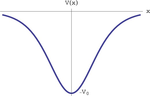
Fig. 3.
A potential well |$V(x)=-V_0g(x/a)$| of depth |$V_0$|.
Setting
|$f(z)=|e|-g(z)$|, if
|$g(z)\to 0$| faster than
|$1/|z|$| for
|$|z|\to\infty$|, then the condition in Eq. (
37) applies. Vanishing the coefficient of the positive exponentials in the solutions in Eqs. (
34) and (
35), we obtain the necessary conditions for a decaying solution at infinity. At the zeroth and first order of
|$g(z)$|, we have
where we defined the quantity
|$\Delta_{\infty} \equiv \int_0^{\infty}g(z)dz$|. Vanishing the determinant of the above system, we have the condition
or, in terms of the energy
|$E$|,
We have recovered the result given on p. 163 of Ref. [29].
We end this section by briefly studying the time evolution of a quantum state. To directly apply the formalism of Sect.
2, we consider the time evolution of
|$\langle\psi(t)|$|. Setting
|$\hbar=1$| for brevity, we have
where
|$H_0$| is a time-independent Hamiltonian and
|$\varepsilon H_1(t)$| is a small time-dependent correction to
|$H_0$|. Passing to the interaction representation [
30], we may always transform Eq. (
48) into
with
|$ H_I(t)=\exp[i H_0 t] H_1(t)\exp[-iH_0t]$|. Using the results of Sect.
2 at
|$\varepsilon$| order, we may write the approximate solution
where the coefficients
|$c_n$| are given by Eq. (
21). Without specifying the commutator
|$[H^{(i)}_I(t),H^{(k)}_I(t)]$|, no further calculations can be performed. Finally, we note that if the perturbation
|$H_1(t)$| is time independent, then the approximate solution for the time evolution of a state
|$|\psi(t)\rangle$| is given by
5. Statistical mechanics and non-linear equations
The analytical solution of a non-linear first-order differential equation is an unsolved problem. There is no general method to solve such a differential equation. One can use a recursive method such as the method of successive approximations (see, for example, Ref. [
31]). These kinds of methods are quite hard to handle from an analytical point of view. In this section, we will provide an approximate closed formula for first-order non-linear differential equations. Let us consider the non-linear first-order equation
where
|$\mathbf{x}$| is a vector and
|$\mathbf{a}(\mathbf{x},t)$| is a given vectorial function. Its connection to statistical mechanics can be found simply by interpreting Eq. (
52) as a Langevin equation [
16,
17]. The corresponding Liouville equation is
If
|$\mathbf{a}(\mathbf{x},t)$| is a stochastic function then, via Van Kampen’s lemma [
18], the Liouvillian density is related to the probability density by the relation
The difficulty of solving Eq. (
52) is inherited by Eq. (
53), since there is also no general method for solving it. But, using physical arguments, if we interpret Eq. (
52) as the motion equation of a particle, then the solution of Eq. (
53) is
where
|$\delta(z)$| is the Dirac delta function and
|$\mathbf{x}_P(t)$| is the solution of Eq. (
52). An important advantage of considering the Liouville equation, or, more generally, a linear partial differential equation, is that for the partial differential equation we may use a linear theory. For our purposes, we can exploit the theory developed in Sect.
3. For the sake of simplicity, we shall focus on a one-dimensional case with
|$a(x, t)$| a real function. The one-dimensional case can be related to anomalous diffusion. Over the past 30 years, anomalous diffusion has been intensively investigated [
32–
36]. We will study the following non-linear equation [
24,
37,
38]:
where, in an overdamped regime,
|$V(x)$| represents a potential and
|$F(t)$| can be interpreted as a force (and more generally as a stochastic force). The above equation can always be rewritten as
where now
|$t$|,
|$x$|,
|$v(x)$|, and
|$f(t)$| are dimensionless quantities and
|$\varepsilon$| is a parameter that we will take to be small. The corresponding Liouville equation is
Due to the formalism developed in Sect.
3 it is more convenient to study the equivalent equation:
Both equations have as solution an arbitrary function
|$G(x,t)=\mathrm{const.}$|, where the arguments
|$x,t$| are the solution of the characteristic equation, i.e. Eq. (
57). Knowledge of the characteristic curve implies knowledge of the function
|$x_P(t)$| of Eq. (
55), and ultimately knowledge of the statistical function
|$\rho(x,t)$|. Following the prescription of Sect.
2, a formal solution of Eq. (
59) via Eq. (
9) is given by
with the understanding that the partial derivative with respect to
|$x$| acts on the left (stressed by the arrow on top of the partial derivative symbol), while the partial derivative with respect to
|$t$| acts on the right. It is straightforward to verify that the derivative of the operator
|$M(t)=\varepsilon [v'(x)-f(t)] \partial_x$| commutes with all its higher-order derivatives, i.e.
Applying Eq. (
29), we obtain the approximate solution
To perform the action of the exponential operators we make a change of variable:
and we have
where we used the definition of
|$\Delta(u)$| given in Eq. (
36). We may rewrite Eq. (
62) as
With sufficient accuracy, we may substitute the partial derivative
|$\partial_{w}$| with
|$\partial_{u}$|. Integrating by parts, taking into account that
|$\bar{\Phi}\left[w(x-\varepsilon \Delta(t) )+ t \right]|_{t=0}= \bar{\Phi}(w(x))=\Phi(x,0) $|, we finally obtain
The solution of the linear problem gives us the solution of the non-linear problem in Eq. (
57), setting as constant the argument of the function
|$ \bar{\Phi}(z)$|, i.e.
The constant can be determined using the initial condition |$x=x_0$| at |$t=0$|.
It is worth stressing the following points:
(1) In principle the method can be applied to higher-order differential equations. The amount of calculation increases considerably, and this is left for future work.
(2) When |$f(t)$| is a constant, Eq. (67) gives the known exact solution.
(3) The difficulties in inverting Eq. (67) with respect to |$x$| are the same as the exact case, i.e. when |$f(t)=\mathrm{const}$|.
(4) The derivative of the potential function |$v'(x)$| is subjected to the less restrictive condition |$|v'(x)|< K$| with |$K$| a positive constant, while |$f(t)$| must satisfy the stricter condition in Eq. (37).
We will now consider an example that will illustrate points (2), (3), and (4). We will study Eq. (
67) using a periodic potential, that does not satisfy Eq. (
37), in the presence of an arbitrary force
|$f(t)$|. This problem is known as the “diffusion in the egg carton” potential [
39,
40]. The movement equation is
According to Eq. (
67), the solution of Eq. (
68) is given by
The inversion of Eq. (
69) is straightforward, and
|$x(t)$| can be found explicitly as
We point out that
|$f(t)$| is a generic function satisfying the condition in Eq. (
37). In particular,
|$f(t)$| could be a stochastic function such as dichotomous noise. Taking the average of Eq. (
55), where
|$x_P(t)$| is given by Eq. (
70), via Eq. (
54), we may obtain the distribution density
|$P(x,t)$|. We briefly consider a symmetric dichotomous noise
|$f(t)=\pm W$|, and we have
The average is taken over infinitely many realizations of the density, and it depends on the correlation function
|$\langle f(t)f(t')\rangle$|. For more details we refer the reader to specialized publications (see, for example, Ref. [
41] and the references therein). Finally, we check the solution in Eq. (
70) in the case of a slowly damped harmonic force
|$f(t)$|,
In Fig. 4 we compare the numerical and the analytical solution. The agreement is excellent and the percent error evaluated with the formula in Eq. (39) is smaller than |$1\%$|. A detailed study of the solution is outside the scope of this paper.
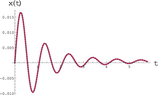
Fig. 4.
The dotted line represents the numerical solution of Eq. (68), while the continuous line is the solution in Eq. (70). The values of the parameters are: |$a=-1$|, |$\beta=2$|, |$f_0=1$|, |$b=1$|, |$ \Omega = 6$|, |$ \tau = 1$|, |$ \varepsilon = 0.1$|.
6. Conclusion
In this paper, we have shown how to determine two coefficients in the Zassenhaus expansion. The analytical expression of these coefficients allowed a series of applications ranging from |$n$|th-order linear equations to evaluation of eigenvalues and first-order non-linear equations. We have been able to build an approximate closed formula at first order of the expansion parameter |$\varepsilon$| in the case of linear differential equations and non-linear first-order differential equations. We have shown applications regarding the evaluation of eigenvalues and statistical mechanics. Finally, we have given a formula implying an infinite matrix product of exponential operators for the time evolution of a quantum state. According to the expression of the Hamiltonian, the product of the exponential operators can be summed and expressed as a closed analytical formula. The approach presented could be extended to evaluate other coefficients in the Zassenhaus expansion and to solve higher-order non-linear differential equations. This is left for future work.
Acknowledgements
The author acknowledges financial support from UTA Mayor project No. 8731-15 and Phy.C.A for logistical support.
References
[1]Campbell
J. E.
,
Proc. London Math. Soc.
s1-29
,
14
(
1897
). ()
[2]Baker
H. F.
,
Proc. London Math. Soc.
(second series)
s2-3
,
24
(
1905
). ()
[3]Hausdorff
F.
,
Leipziger Ber
.
58
,
19
(
1906
). ()
[4]Magnus
W.
,
Comm. Pure Appl. Math.
7
,
649
(
1954
). ()
[5]Quesne
C.
,
Intern. J. Theo. Phys.
43
,
545
(
2004
). ()
[6]Blanes
S.
, Casas
F.
, Oteo
J. A.
, and Ros
J.
,
Phys. Rep.
470
,
151
(
2009
). ()
[7]Kimura
T.
,
Prog. Theor. Exp. Phys.
2017
,
041A03
(
2017
). ()
[8]Sato
K.
,
Prog. Theor. Exp. Phys.
2017
,
123D03
(
2017
). ()
[9]Marconi
U. M. B.
and Corberi
F.
,
Europhys. Lett.
30
,
349
(
1995
). ()
[10]Pedrosa
I. A.
and Rosas
A.
,
Phys. Rev. Lett.
103
,
010402
(
2009
). ()
[11]Quan
H. T.
and Zurek
W. H.
,
New J. Phys.
12
,
093025
(
2010
). ()
[12]Darázs
Z.
and Kiss
, T.
J. Phys. A: Math. Theor.
46
,
375305
(
2013
). ()
[13]Soto-Eguibar
F.
and Moya-Cessa
H. M.
,
Appl. Math. Inf. Sci.
9
,
175
(
2015
). ()
[14]Soloviev
M. A.
,
Phys. Rev. D
94
,
105021
(
2016
). ()
[15]Yatabe
A.
and Yamada
S.
,
Prog. Theor. Exp. Phys.
2018
, 033B04 (2018). ()
[16]Lemons
D. S.
,
Am. J. Phys.
65
,
1079
(
1997
). ()
[17]Bao
J.-D.
, Zhuo
, Y.-Z.
Oliveira
, F. A.
and Hänggi
, P.
Phys. Rev. E
74
,
061111
(
2006
). ()
[18]Van Kampen
N. G.
,
Phys. Rep.
24
,
171
(
1976
). ()
[19]West
B. J.
,
Applied Stochastic Processes
(
Academic Press
,
New York
,
1980
), p.
283
.
[20]Bianucci
M.
, Mannella
R.
, Grigolini
P.
, and West
B. J.
,
Int. J. Mod. Phys. B
8
,
1191
(
1994
). ()
[21]Bianucci
M.
, Mannella
R.
, Grigolini
P.
, and West
B. J.
,
Int. J. Mod. Phys. B
8
,
1211
(
1994
). ()
[22]Bianucci
M.
, Mannella
R.
, Grigolini
P.
, and West
B. J.
,
Int. J. Mod. Phys. B
8
,
1225
(
1994
). ()
[23]Wang
L.
, Li
, N.
and Hänggi
, P.
Thermal transport in low dimensions: From statistical physics to nanoscale heat transfer
, in
Lecture Notes in Physics
, ed.
Lepri
S.
(
Springer-Verlag
,
Berlin
,
2016
), Vol.
921
, p.
239
.
[24]Bianucci
M.
,
J. Math. Phys.
59
,
053303
(
2018
). ()
[25]West
B. J.
,
Fractional Calculus View of Complexity: Tomorrow’s Science
(
CRC Press
,
Boca Raton, FL
,
2016
).
[26]Turalska
M.
and West
B. J.
,
Chaos Solitons Fract.
102
,
387
(
2017
). ()
[27]Bologna
M.
,
Eur. Phys. J. Plus
131
,
386
(
2016
). ()
[28]Scholz
D.
and Weyrauch
M.
,
J. Math. Phys.
47
,
033505
(
2006
). ()
[29]Landau
L. D.
and Lifshitz
E. M.
,
Quantum Mechanics Non-Relativistic Theory
(
Pergamon Press
,
Oxford
,
1991
), 3rd ed.
[30]Landau
L. D.
and Lifshitz
E. M.
,
Quantum Electrodynamics
(
Pergamon Press
,
Oxford
,
1982
), 2nd ed.
[31]Kelley
W. G.
and Peterson
A. C.
.
The Theory of Differential Equations
(
Springer
,
New York
,
2010
).
[32]Bouchaud
J.-P.
and Georges
A.
,
Phys. Rep.
195
,
127
(
1990
). ()
[33]Metzler
R.
and Klafter
J.
,
Phys. Rep.
339
,
1
(
2000
). ()
[34]Zaslavsky
G. M.
,
Phys. Rep.
371
,
461
(
2002
). ()
[35]Bologna
M.
and Aquino
G.
,
Eur. Phys. J. B
87
,
15
(
2014
). ()
[36]Spiechowicz
J.
, Łuczka
, J.
and Hänggi
, P.
Sci. Rep.
6
,
30948
(
2016
). ()
[37]Sancho
J. M.
and San Miguel
M.
,
Prog. Theor. Phys.
69
,
1085
(
1983
). ()
[38]Sancho
J. M.
,
J. Math. Phys.
25
,
354
(
1984
). ()
[39]Caratti
G.
, Ferrando
R.
, Spadacini
R.
, and Tommei
G. E.
,
Physica A
246
,
115
(
1997
). ()
[40]Caratti
G.
, Ferrando
R.
, Spadacini
R.
, and Tommei
G. E.
,
Phys. Rev. E
55
,
4810
(
1997
). ()
[41]Bologna
M.
and Grigolini
P.
,
J. Stat. Mech.
2009
,
P03005
(
2009
). ()
© The Author(s) 2019. Published by Oxford University Press on behalf of the Physical Society of Japan.
This is an Open Access article distributed under the terms of the Creative Commons Attribution License (
http://creativecommons.org/licenses/by/4.0/), which permits unrestricted reuse, distribution, and reproduction in any medium, provided the original work is properly cited.


