Extension of photon surfaces and their area: Static and stationary spacetimes

Abstract

1. Introduction

In a Schwarzschild spacetime, a collection of unstable circular orbits of null geodesics forms a sphere at |$r=3GM$|⁠, called a photon sphere. The photon sphere plays an important role in phenomena related to observations, like gravitational lensing [5] and the ringdown of waves around a black hole [6]. The region between the event horizon and the photon sphere is a very characteristic region because if photons are emitted isotropically from a point in this region, more than half of them will be (eventually) trapped by the horizon [7] (see also Sect. 5.1 of Ref. [8]).

Here, |$A_0$| is the area of a surface in the strong gravity region and the right-hand side is the area of the photon sphere of a Schwarzschild spacetime with the same mass. In this paper, we call this inequality the Penrose-like inequality. In order to formulate and prove the Penrose-like inequality, we have to introduce an appropriate concept of a surface characterizing the strong gravity region.

One of the generalized concepts of the photon sphere is the photon surface [9]. It is defined as a timelike hypersurface |$S$| such that any photon emitted in any tangent direction of |$S$| from any point on |$S$| continues to propagate on |$S$|⁠. The photon surface is allowed to be dynamical or to be non spherically symmetric. In our context, the concept of the static photon surface may be expected to be useful to characterize the strong gravity region. However, the existence of a photon surface practically requires high symmetry of the spacetime, because the condition of a photon surface strongly constrains the photon behavior on it. For this reason, the uniqueness of static photon surfaces has been expected and partially proved [10–19]; if a static photon surface exists, the spacetime must be spherically symmetric in various setups (see also an example of a nonspherical photon surface but with a conical singularity [20]). Another manifestation of the strong requirement on a photon surface is that it does not exist in stationary spacetimes. In a Kerr spacetime, for example, there are null geodesics staying on |$r=\mathrm{const.}$| surfaces, but their |$r$| values depend on the angular momentum of the photons [21]. As a result, a collection of photon orbits with constant |$r$| values forms a photon region with thickness instead of a photon surface (Sect. 5.8 of Ref. [8]). The photon region becomes infinitely thin and reduces to a photon surface in the limit of zero rotation.

Clearly, the absence of a photon surface does not imply the absence of a strong gravity region. It is nice to introduce other concepts to characterize the strong gravity region that are applicable to spacetimes without high symmetry or to stationary spacetimes. One such approach is the loosely trapped surface (LTS) proposed by us gravity region that are applicable to spacetimes without high[22]. An LTS is defined with quantities of intrinsic geometry of the initial data; in a Schwarzschild spacetime, the marginal LTS coincides with the photon sphere. We have proved that LTSs satisfy the Penrose-like inequality (2) in initial data with a nonnegative Ricci scalar. However, the connection between the LTS and the photon behavior in non-Schwarzschild cases is still unclear. We speculated that such a connection would exist, but it was left as a remaining problem.

In light of the above discussion, the purpose of this paper is threefold. First, as a generalization of the static photon surface, we introduce a new concept to characterize a strong gravity region through the behavior of photons, the transversely trapping surface (TTS). A TTS is defined as a static/stationary timelike hypersurface |$S$| such that arbitrary photons emitted tangentially to |$S$| propagate on or toward the inside of |$S$|⁠. TTSs can be present in static spacetimes without high symmetry and in stationary spacetimes, and examples in a Kerr spacetime are explicitly calculated. Second, we show how the TTS is related to the LTS in static spacetimes and axisymmetric stationary spacetimes. Through this study, we give an answer to the remaining problem of our previous paper. Third, we will prove that TTSs satisfy the Penrose-like inequality (2) in static spacetimes and axisymmetric stationary spacetimes under fairly generic conditions.

This paper is organized as follows. In the next section, we explain the basic concepts and properties of the TTS and the LTS. In Sect. 3, we study TTSs in static spacetimes. In Sect. 4, TTSs in axisymmetric stationary spacetimes are explored. Section 5 is devoted to a summary and discussion. In Appendix A, we present derivations of the TTS condition in static and axisymmetric-stationary cases in a different manner from those in the main article. In Appendix B, we give a supplementary explanation of the derivation of the TTS condition in the axisymmetric stationary case. In Appendix C, we present some geometric formulas that are useful for studying TTSs in more general cases. Throughout the paper, we use units in which |$c=1$|⁠. Although we write the Newton constant |$G$| basically, we set |$G=1$| when a Kerr spacetime is studied in Sect. 4.2 for conciseness.

2. Definitions of surfaces in strong gravity regions

In this section, we explain the two concepts of surfaces to characterize strong gravity regions. In Sect. 2.1, we define the TTS and derive the mathematical condition for a surface |$S$| to be a TTS. In Sect. 2.2, we review the LTS introduced in our previous paper [22]. A theorem proved in Ref. [22], which is used in this paper as well, is also reviewed.

2.1. Transversely trapping surfaces

Consider a static or stationary spacetime |$\mathcal{M}$| possessing a timelike Killing vector field |$t^a$|⁠, and take a spacelike hypersurface |$\Sigma$| given by |$t=\mathrm{const.}$| We consider an orientable closed two-surface |$S_0$| in |$\Sigma$| and suppose that |$\Sigma$| is divided into the inside and outside regions by |$S_0$|⁠. By transporting |$S_0$| along the integral lines of |$t^a$|⁠, we obtain a static/stationary three-dimensional timelike surface |$S$|⁠. In this setup, we define the TTS as follows:

Below, we derive the mathematical expression for the condition for |$S$| to be a TTS. Before starting our analysis, we summarize the notations commonly used throughout this paper. The metric of the spacetime |$\mathcal{M}$| is |$g_{ab}$|⁠. With the future-directed unit normal |$n^a$| to |$\Sigma$|⁠, the induced metric and the extrinsic curvature of |$\Sigma$| are given by |$q_{ab}=g_{ab}+n_an_b$| and $Kab=(1/2)£nqab$⁠, respectively, where $£$ denotes the Lie derivative. With the outward unit normal |$\hat{r}^a$| to |$S$|⁠, the induced metric and the extrinsic curvature of |$S$| are |$P_{ab}=g_{ab}-\hat{r}_a\hat{r}_b$| and $K¯ab=(1/2)£r^Pab$⁠, respectively. Although the unit normal to |$S$| in |$\mathcal{M}$| and the unit normal to |$S_0$| in |$\Sigma$| do not coincide in general, in this paper we consider setups such that these two unit normals agree. We will come back to this point in Sects. 3.1 and 4.1. In this situation, the induced metric of |$S_0$| is |$h_{ab}=g_{ab}+n_an_b-\hat{r}_a\hat{r}_b$|⁠, and its extrinsic curvature in the hypersurface |$\Sigma$| is $kab=(1/2)(3)£r^hab$⁠, where $(3)£$ is the Lie derivative on the hypersurface |$\Sigma$|⁠. The covariant derivatives of |$\mathcal{M}$|⁠, |$\Sigma$|⁠, |$S$|⁠, and |$S_0$| are denoted as |$\nabla_a$|⁠, |$D_a$|⁠, |$\bar{D}_a$|⁠, and |$\mathcal{D}_a$|⁠, respectively. These definitions are summarized in Fig. 1.

Fig. 1.

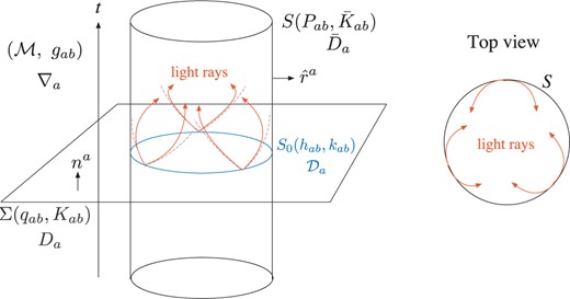
Schematic picture of the transversely trapping surface. The notations are also indicated.

Open in new tabDownload slide

Hereafter, we call this condition the TTS condition. In Sects. 3.1 and 4.1, we will rewrite the TTS condition in the cases of static spacetimes and axisymmetric stationary spacetimes. Note that if the equality in Eq. (5) holds at all points on |$S$|⁠, the surface |$S$| coincides with the photon surface proposed in Ref. [9]. Therefore, our definition of the TTS includes the photon surface as the marginal case.

In addition to the TTS condition, we sometimes require the two-surface |$S_0$| to be a convex surface. The condition for the convexity depends on the choice of the slice |$t=\mathrm{const}.$| We will specify this point in Sects. 3.1 and 4.1. When the convex condition is additionally imposed on the TTS, we call it the convex TTS.

2.2. Loosely trapped surfaces

Now, we explain the LTS defined in our previous paper [22]. Consider the initial data |$\Sigma$| of a (not necessarily static or stationary) spacetime |$\mathcal{M}$| and a closed two-surface |$S_0$| that divides |$\Sigma$| into outside and inside regions. The initial data |$\Sigma$| is supposed to have a nonnegative Ricci scalar |${}^{(3)}R\ge 0$|⁠. We introduce a radial foliation of |$\Sigma$| starting from |$S_0$| specified by the coordinate |$r$| with the dual basis |$D_ar=\hat{r}_a/\varphi$|⁠, where |$\hat{r}_a$| is the unit normal to |$S_0$| and |$\varphi$| is the (spatial) lapse function. In this setup, the LTS is defined as follows:

This is proved by integrating the relation (6) under the condition |$\hat{r}^aD_ak\ge 0$| and |${}^{(3)}R\ge 0$|⁠, and using the Gauss–Bonnet theorem. The second result is very important in this paper, and we state it in the form of a theorem:

In order to prove this, we used the method of the inverse mean curvature flow originally proposed in Refs. [2, 23]. The inverse mean curvature flow is generated by the lapse function |$\varphi=1/k$|⁠, and along this flow, Geroch’s quasilocal energy is monotonic and asymptotes to the ADM mass at spacelike infinity |$r\to \infty$|⁠.¹ This leads to the bound on the surface area (see also Ref. [3] for resolution of the possible formation of singularities along the flow). We refer to our previous paper [22] for the detailed proof. Note that the theorem in Ref. [22] states that the Penrose-like inequality holds for an LTS. We modified the statement of the theorem to the above because the inequality (7) and |$k\ge 0$| on |$S_0$| are necessary in the proof, but the LTS condition |$\hat{r}^aD_ak\ge 0$| is not used directly; it was used to guarantee (7) in our previous paper. This modification will become important in Sects. 3.3 and 4.4.

3. Static spacetimes

In this section, we explore the properties of TTSs in static spacetimes. In Sect. 3.1, we explain the setup and rewrite the TTS condition. In Sect. 3.2, the relation between the TTS and the LTS is examined using the Einstein equations. The Penrose-like inequality for TTSs is proved in Sect. 3.3.

3.1. Setup and TTS condition

As defined in Sect. 2.1, we call |$S$| a convex TTS when |$S_0$| is a convex surface. The surface |$S_0$| is a convex surface if and only if both |$k_1$| and |$k_2$| are nonnegative. Therefore, for |$S$| to be a convex TTS, we require |$k_2\ge 0$| in addition to the condition (15). The convex condition can also be expressed in a covariant manner as |$k\ge \sqrt{2\tilde{k}_{ab}\tilde{k}^{ab}}$|⁠.

3.2. Connection to the LTSs

Therefore, we have found the following:

Note that the condition |$\rho+P_r=0$| is not too strong because it must be imposed just on |$S$| and it is satisfied if the region around |$S$| is vacuum. Also, the Reissner–Nordström spacetimes satisfy this condition for |$r=\mathrm{const.}$| surfaces. In this sense, we have proved the close connection between the TTS and the LTS with sufficient generality.

3.3. Area bound for TTSs

Once a TTS is proved to be an LTS, it possesses the properties that have been proved for LTSs. In particular, its area satisfies the Penrose-like inequality (2), |$A_0\le 4\pi (3GM)^2$|⁠. However, there might be the case that a TTS is not guaranteed to be an LTS but satisfies the Penrose-like inequality (i.e., we suppose that |$\rho+P_{r}=0$| may not be necessary on |$S$|⁠). Therefore, there remains a possibility that the condition can be relaxed if just the area bound is considered. Let us explore this possibility.

If |$k>0$| at least at one point, the Gauss–Bonnet theorem tells us that |$S_0$| has topology |$S^2$| and the left-hand side is |$\int{}^{(2)}RdA=8\pi$|⁠. This implies the inequality (7). Therefore, we have found the following:

Compared to Proposition 2 in Sect. 3.2, the equality |$\rho+P_r=0$| is relaxed to the inequality |$P_r\le 0$|⁠. Therefore, Theorem 2 is expected to have greater applicability. Note that from Eq. (25), this theorem also holds for a nonconvex TTS if |$k_2$| is within the range |$k_2\ge -k_1/3$|⁠.

4. Axisymmetric stationary spacetimes

In this section, we explore the properties of axisymmetric TTSs in (nonstatic) stationary spacetimes with axial symmetry. In Sect. 4.1, we explain the setup in detail and rewrite the TTS condition. In Sect. 4.2, we show that TTSs actually can exist in a stationary spacetime by presenting examples of a Kerr spacetime. In Sect. 4.3, the relation between the TTS and the LTS is examined, but for fairly restricted situations. The Penrose-like inequality for the TTS is proved in Sect. 4.4.

4.1. Setup and TTS condition

Physically, this condition means that matter, if it exists, is moving just in the |$\phi^a$| direction. In this case, there exists the symmetry of the metric under the transformation |$t^a\to -t^a$| and |$\phi^a\to -\phi^a$|⁠.

Here, the quantity |$\omega$| in Eq. (29) corresponds to the angular velocity of the zero-angular-momentum observers (ZAMOs). Note that this condition is realized only on a special slice. For example, although the Boyer–Lindquist coordinates of the Kerr spacetime possess this property, other coordinates like the Kerr–Schild coordinates [29] or the Doran coordinates [30] do not satisfy this condition because the shift vector has a radial component.

In this paper, we consider only axisymmetric TTSs for a technical reason. If a TTS |$S$| is axisymmetric, the timelike unit normal |$n^a$| to |$\Sigma$| becomes a tangent vector of |$S$|⁠, because both |$t^a$| and |$\beta^a$| are tangent to |$S$|⁠. Then, the outward unit normal |$\hat{r}^a$| to |$S$| becomes the outward unit normal to |$S_0$| in |$\Sigma$| as well. If |$S$| is not axisymmetric, these properties do not hold and the analysis becomes complicated. The study of nonaxisymmetric TTSs in the stationary case is left as a remaining problem.

Similarly to the static case, this condition can be derived by directly studying the geodesic equations. This is demonstrated in Appendix A.2. For a convex TTS, the conditions |$k_1\ge 0$| and |$k_2\ge 0$| are additionally required.

4.2. Examples in a Kerr spacetime

Here, |$M$| is the ADM mass and |$a$| is the rotation parameter that is related to the ADM angular momentum as |$J=Ma$|⁠. The event horizon is located at |$r=r_+=M+\sqrt{M^2-a^2}$|⁠. We consider the parameter region |$0<a\le M$|⁠, i.e., a nonstatic spacetime with an event horizon.

The behavior of |$r^{\rm (TTS)}_{\rm max}$| is shown as a function of |$a/M$| in Fig. 2. Note that the value of |$r^{\rm (TTS)}_{\rm max}$| corresponds to the radius of the circular orbit of a photon closest to the black hole (e.g., p. 73 of Ref. [31]). Therefore, our result is reasonable because only photons propagating on the equatorial plane in the direction of the black hole rotation propagate on the surface |$r=r^{\rm (TTS)}_{\rm max}$|⁠, and all other photons initially moving in the tangent direction to the surface will fall into the black hole.

Fig. 2.

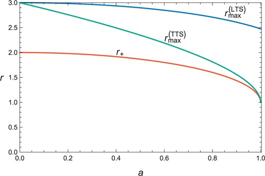
The behavior of |$r^{\rm (TTS)}_{\rm max}$| and |$r^{\rm (LTS)}_{\rm max}$| as functions of |$a$|⁠. The unit of the length is |$M$|⁠.

Open in new tabDownload slide

Let us also look at LTSs in the Kerr spacetime. A surface |$r=\mathrm{const.}$| becomes an LTS when |$k_{,r}\ge 0$| is satisfied at every point. This condition becomes strictest on the equatorial plane |$\theta=\pi/2$|⁠, and there exists a maximum radius |$r^{\rm (LTS)}_{\rm max}$| such that an |$r=\mathrm{const}.$| surface becomes an LTS for |$r_+\le r\le r^{\rm (LTS)}_{\rm max}$|⁠. Unfortunately, no simple analytic formula for |$r^{\rm (LTS)}_{\rm max}$| seems to exist, unlike the TTS case. The behavior of |$r^{\rm (LTS)}_{\rm max}$| is shown in Fig. 2. Although |$r^{\rm (LTS)}_{\rm max}=r^{\rm (TTS)}_{\rm max}=3M$| at |$a/M=0$|⁠, LTSs distribute in a broader region compared to TTSs when |$a/M$| is large. While |$r=r^{\rm (TTS)}_{\rm max}$| indicates the inner edge of the photon region, |$r=r^{\rm (LTS)}_{\rm max}$| is located in the middle of the photon region. In this sense, the TTS and the LTS are different indicators for strong gravity regions, and the TTS is a stricter one compared to the LTS.

4.3. Connection to the LTSs

Fig. 3.

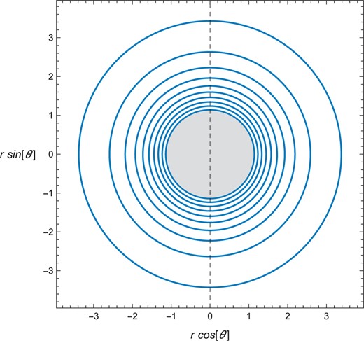
Contour surfaces of the ZAMO angular velocity |$\omega$| for |$\omega/\Omega_{\rm H}=n/10$| with |$n=1,\ldots,10$|⁠, where |$\Omega_{\rm H}$| is the angular velocity of the event horizon, in the |$(r\cos\theta,r\sin\theta)$|-plane of a Kerr spacetime with |$a/M=0.99$|⁠. The unit of the length is |$M$|⁠.

Open in new tabDownload slide

Compared to the static case, the argument here is fairly restricted, not because a convex TTS is not an LTS in many situations, but because the method here does not work sufficiently. As we have seen in the Kerr case, the TTSs given by |$r=\mathrm{const}.$| surfaces are simultaneously LTSs for all |$0\le a/M\le 1$|⁠. We expect that a better method may establish the connection between the TTS and the LTS in the axisymmetric stationary case more firmly. This is left as a remaining problem.

4.4 Area bound for TTSs

If the right-hand side is positive, |$S_0$| has topology |$S^2$| and the left-hand side becomes |$\int_{S_0}{}^{(2)}RdA=8\pi$| because of the Gauss–Bonnet theorem. Therefore, we have the following result:

Here, we discuss to what extent the condition (58) is strong. Since |$\phi^a\mathcal{D}_a\omega=0$|⁠, the right-hand side is rewritten as |$(\hat{\theta}^aD_a\omega)^2$|⁠. This quantity is zero at the symmetry axis, and also on an equatorial plane (if it exists). Therefore, the condition (58) is satisfied at least at these two locations. Furthermore, since the ZAMO angular momentum |$\omega$| coincides with the (constant) horizon angular velocity |$\Omega_{\rm H}$| on the event horizon, the condition (58) must be satisfied at least on surfaces sufficiently close to the event horizon. For this reason, the condition (58) does not restrict the situation strongly, and hence many TTSs satisfying this condition should exist. In fact, we can check that this condition is satisfied by arbitrary |$r=\mathrm{const.}$| surfaces of a Kerr spacetime. Therefore, Theorem 3 is expected to have sufficient generality.

5. Summary and discussion

In this paper, we have defined a new concept, the transversely trapping surface, as a generalization of static photon surfaces. Its definition was introduced in Sect. 2.1 (Definition 1), and the condition for a surface |$S$| to be a TTS is mathematically expressed as Eq. (5) in Proposition 1. The properties of the TTS in static spacetimes were studied in Sect. 3. There, a TTS is proved to be a loosely trapped surface as defined in our previous paper [22] (see Definition 2 of this paper) at the same time under certain conditions (Proposition 2 in Sect. 3.2). The area of a TTS is shown to satisfy the Penrose-like inequality (2) under some generic conditions (Theorem 2 in Sect. 3.3).

In Sect. 4, we studied TTSs in axisymmetric stationary spacetimes. Because of a technical reason, we considered axisymmetric TTSs in spacetimes with the |$t$|–|$\phi$| orthogonality property. The TTS condition in this setup was summarized in a concise form (Proposition 3 in Sect. 4.1). It was explicitly shown that TTSs exist in a Kerr spacetime (Sect. 4.2). As for the connection to the LTS, we have shown that TTSs given by contour surfaces of the ZAMO angular velocity are LTSs at the same time under certain conditions (Proposition 4 in Sect. 4.3). This fairly restricted argument is due to a technical reason, and generalization is left as an open problem. However, we have proved the Penrose-like inequality (2) under fairly general situations (Theorem 3 in Sect. 4.4).

We have established that the area of a TTS is bounded from above by the area of a photon sphere with the same mass in quite generic static/stationary situations. This is a natural result, because if photons propagating in the transverse direction to the source are trapped, such a region must be compact so that gravity is sufficiently strong.

It is interesting to list spacetimes possessing TTSs. Black hole spacetimes generally possess TTSs around their horizons. In addition to the vacuum black holes, black holes surrounded by ring-shaped matter [32] and those with scalar or proca hairs [33–35] also possess TTSs. There are a few examples of spacetimes without horizons where TTSs are present. One is a spherically symmetric star composed of incompressible fluid (e.g., Ref. [25]): the radius of such a star |$R$| can be as small as |$8/3\le R/M\le 3$| without violating the dominant energy condition. Another example is the soliton-like structure of a complex massive scalar field, the so-called boson star. It has been reported in Ref. [36] that a boson star can have a photon sphere (and, therefore, TTSs), although the binding energy is not negative for such situations if the scalar field is minimally coupled to gravity. Other rather exotic examples are spacetimes with naked singularities, as studied in Refs. [37–41].

In this paper, we restricted the definition of the TTS as a static/stationary surface in a static/stationary spacetime. It would be possible to generalize this definition to more general surfaces in dynamical spactimes. For example, one may define the generalized TTS as an arbitrary spatially bounded timelike surface |$S$| on which the TTS condition |$\bar{K}_{ab}k^ak^b\le 0$| holds for arbitrary null tangent vectors |$k^a$| everywhere. Taking account of this possibility, in Appendix C we present some useful geometric formulas in the setup given by Fig. 1 but without assuming the timelike Killing symmetry. As special cases, the formulas in the main text are rederived as a consistency check.

Second, there is another formulation for compactness of an apparent horizon, the hoop conjecture [44], which states that black holes with horizons form when and only when a mass |$M$| gets compacted into a region whose circumference in every direction is bounded by |$C\lesssim 2\pi (2GM)$|⁠. The important claim of this conjecture is that an apparent horizon does not become arbitrarily long in one direction, and this property was shown to hold in several examples (e.g., Ref. [45]). It would be interesting to test whether TTSs also satisfy this property. We expect that an argument such that the circumference of a TTS is bounded as |$C\lesssim 2\pi (3GM)$| could be made.

Finally, since a TTS suggests that gravity is strong there, ordinary matter would not be able to support itself inside of the TTS. Therefore, it would be possible to show the existence of a horizon inside of a TTS under some conditions. In the spherically symmetric case, it has been shown that a perfect fluid star consisting of polytropic balls cannot possess a photon sphere [46]. We expect that it would be possible to generalize such an argument for nonspherical TTSs applying the methods for proving singularity theorems.

Acknowledgements

The work of H. Y. was in part supported by a Grant-in-Aid for Scientific Research (A) (No. 26247042) from the Japan Society for the Promotion of Science (JSPS). K. I. is supported by a JSPS Grant-in-Aid for Young Scientists (B) (No. 17K14281). T. S. is supported by a Grant-in-Aid for Scientific Research (C) (No. 16K05344) from JSPS.

Appendix A. TTS conditions from geodesic equations

The purpose of this appendix is to demonstrate that the TTS conditions in the static case and in the axisymmetric stationary case can be derived by directly examining the geodesic equations.

A.1. Static spacetimes

A.2. Axisymmetric stationary spacetimes

Therefore, this function |$f(x)$| must be nonnegative in the interval |$[-1,1]$|⁠. Using the relation (40) between the tetrad components of |$k_{ab}$| and |$v_a$| and the metric functions, we find that the function |$f(x)$| here is exactly equivalent to Eq. (37) or Eq. (B.1).

Appendix B. Derivation of the conditions (38a)–(38c)

The condition can be studied by dividing it into the three cases as indicated in Fig. B.1:

Fig. B.1.

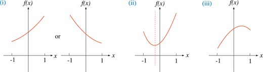
The three cases (i)–(iii) that |$f(x)$| becomes nonpositive in the region |$-1\le x\le 1$|⁠.

Open in new tabDownload slide

• (i) The case that |$k_2> k_1$| and there is no axis in the interval |$[-1,1]$|⁠, i.e., |$|x_{\rm a}|> 1$|⁠. Since |$f(x)$| takes the minimum value at one of the endpoints, we require |$f(\pm 1)\ge 0$|⁠. This leads to the condition (38a).

• (ii) The case that |$k_2> k_1$| and the axis exists in the interval |$[-1,1]$|⁠, i.e., |$|x_{\rm a}|\le 1$|⁠. Since |$f(x)$| takes the minimum value at the axis, we require |$f(x_{\rm a})\ge 0$|⁠. This leads to the condition (38b).

• (iii) The case that |$k_2\le k_1$|⁠. Since |$f(x)$| takes the minimum value at one of the endpoints, we require |$f(\pm 1)\ge 0$|⁠. This leads to the condition (38c).

Appendix C. Useful geometric formulas

In Sects. 3 and 4, we discussed the connection between the TTS and the LTS and the area bound of TTSs for (i) static and (ii) stationary and axisymmetric cases separately. In this appendix, we will present some useful formulas that have a unified treatment for them and the potential for further generalization to dynamical cases. We can also see the role of the assumption of staticity/stationarity in the argument of the main text.

Here, the setup depicted by Fig. 1 is considered. Specifically, the unit normal |$n^a$| to the spacelike hypersurface |$\Sigma$| is tangent vectors of |$S$|⁠, and the outward unit normal |$\hat{r}^a$| to |$S$| is tangent to |$\Sigma$|⁠. First, we derive the general formula without assuming |$t^a$| to be a Killing field or |$t^a$| to be tangent to |$S$| (unlike the main text of this paper); the discussion here also holds for dynamical setups as long as the above conditions are satisfied. After that, the static case and the axisymmetric stationary case are considered. We also note that the study here concerns the relations between geometric quantities, and the field equations are not explicitly imposed. In addition to the quantities in Fig. 1, we introduce one more geometric quantity, that is, the extrinsic curvature |$\bar{k}_{ab}$| of |$S_0$| in the hypersurface |$S$| as defined by $k¯ab=(1/2)£^nhab$⁠. Here, $£^$ denotes the Lie derivative in the timelike hypersurface |$S$|⁠.

C.1 Useful formulas for consideration on LTS

Below, we look at the static case and the stationary axisymmetric case, one by one.

C.1.1. Static case

This corresponds to Eq. (22) when the Einstein equation holds.

C.1.2. Stationary and axisymmetric case