


Abstract
We have measured the cosmic muon flux in the zenith angle range |${<}$| cos |$\theta $||${<}$| 0.37 with a detector comprising planes of scintillator hodoscope bars and iron blocks inserted between them. The muon ranges for up to 9.5 m-thick iron blocks allow the provision of muon flux data integrated over corresponding threshold momenta up to 11.6 GeV/c. Such a dataset covering the horizontal direction is extremely useful for a technique called muon radiography, where the mass distribution inside a large object is investigated from the cosmic muon distribution measured behind the object.
1. Introduction
As the long-term settlement procedure of the Fukushima Daiichi reactor accident has progressed, evaluating the status of nuclear fuels has become one of the key issues to provide information for working on the delicate and complicated fuel removal process. Muon radiography uses cosmic muons to study the inner structure of large objects [1]. The prime advantage of this method is that the structure inside could be imaged from outside, so the accessibility issue of the high-radiation area will not limit the application of this method.
Although the detector system would be located near the large object, in the case of the reactor building of Fukushima Daiichi, the target is far from the detector, and we must use cosmic muons traversing along nearly the horizontal direction. A detailed measurement of muon flux in the zenith angle range 68|$^{\circ}$| to 82|$^{\circ}$| (0.139 |${<}$| cos |$\theta $||${<}$| 0.375) is available [2] for the minimum muon momentum of 1 GeV/c. For muon radiography, muons with momentum below 1 GeV/c and the lower zenith angle range make an important contribution in estimating the mass density inside the building. We therefore carried out a measurement at KEK, High-Energy Accelerator Research Organization, to cover this region using the tracking systems [3] developed for the fuel investigation of the Fukushima Daiichi reactors. Iron blocks with various thicknesses from 0.2 m to 9.5 m are inserted between the tracking planes to provide momentum information based on the muon range in the iron.
2. Experimental setup and data collection periods
2.1. Detector configurations
Figure 1 shows a photograph of the detector system set up in the East Experimental Hall at KEK. There are three tracking units (Unit-1 to Unit-3) with a sensitive cross section of 1 m |$\times$| 1 m that were installed from the beginning of the measurement, and two larger 1.6 m |$\times$| 1.6 m units (Unit-4 and Unit-5) added soon after. To discriminate the muon momentum, the thickness of the iron blocks was varied. The cross-sectional size of the iron block was 1.6 m |$\times$| 1.6 m for 20 cm-thick blocks, and larger than 2 m |$\times$| 2 m for thicker blocks. The relative heights of the tracking units and the iron blocks were modified three times in the measurement period to cover a wider muon zenith angle range. The three detector layouts are illustrated in Fig. 2. The iron blocks shown in the illustrations are typical, and data with other iron block configurations, including the no-iron case, were taken in the same detector layout. The detectors were arranged in the north–south direction, and muons coming from the north were selected using time information available in the detector units. In the following sections, we define the muon track angle as the elevation angle |$\alpha $|, which is related to the zenith angle |$\theta $| as |$\alpha =\pi \mathord{/} 2-\theta $|.
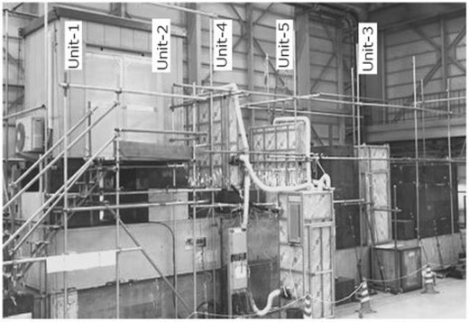
Photograph of a detector setup (Layout-3 with one 2 m iron block inserted in front of Unit-3). Two 1 m |$\times$| 1 m tracking units (Unit-1 and Unit-2) are located inside the storage hut at the top left, with another (Unit-3) behind the iron block at the right end (iron blocks not in use are placed further right). Two 1.6 m |$\times$| 1.6 m units (Unit-4 and Unit-5) are in the middle, where piping for air-conditioning is seen.
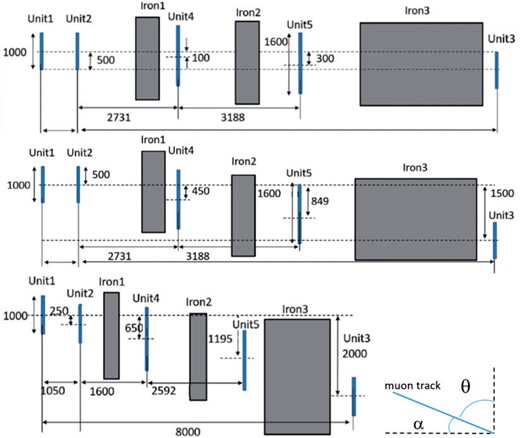
Three detector configurations (dimensions in mm). (Top) Layout-1 to cover the elevation angle range |$0 < \alpha < 118$| mrad (cos |$\theta < 0.118$|). Unit-3 is lowered by 50 cm with respect to Unit-1 and Unit-2. (Middle) Layout-2 to cover the elevation angle range |$39 < \alpha < 196$| mrad (|$0.039 < \text{cos} {}^{\circ}\theta< 0.195$|). Unit-3 is lowered by 1.5 m with respect to Unit-1 and Unit-2. (Bottom) Layout-3 to cover the elevation angle range |$125 < \alpha < 375$| mrad (|$0.125 < \text{cos} \ \theta< 0.366$|). The distance between Unit-1 and Unit-3 is shortened to 8 m.
2.2. The tracking unit
Each of the tracking units comprised a pair of X–Y arrangements of 1 cm-thick scintillating strips of width 1 cm and length 1 m for Unit-1 to Unit-3 [4], and width 4 cm and length 1.6 m for Unit-4 and Unit-5 [5]. The X–Y arrangements were set at 90|$^{\circ}$| from each other to reconstruct the space position point. Therefore, each of Unit-1 to Unit-3 defines the space points in (1 cm)|$^{\mathrm{2}}$| and Unit-4 and Unit-5 in (4 cm)|$^{\mathrm{2}}$|. The scintillator bars were fabricated in extrusion with a hole of approximately 3 mm in diameter at the center, to which a wavelength shifting fiber [6] of 1 mm diameter was inserted to extract scintillator signals from one end of the plane. The four sides of the scintillator bar were coated with TiO|$_{\mathrm{2}}$| and the other end of the fiber with white emulsion paint for light reflection and isolation from neighbors. The readout fiber end was coupled directly to a multi-pixel photon counter (MPPC) [7] with a photo-sensing area of 1.3 mm square.
The 200 signals from each of Units-1–3 were fed into a data acquisition (DAQ) box [3,8]. The DAQ box provided bias voltages to 200 MPPCs, typically 64–71 V, amplified and discriminated the signals, and then examined the hit pattern of 200 signals using FPGAs. The bias voltages and discrimination voltages were remotely adjustable. A total of 160 signals from Unit-4 and Unit-5 were also examined using the same DAQ box. The hit pattern was examined every 8 ns. If hits were found in both X and Y planes within a given time window of 64 ns, the hit scintillator channel pattern and timestamp (1 ns digitization) were transferred to a PC. The clocks among the DAQ boxes were synchronized using a common clock generator.
The physical outer cross-sectional areas were 1.17 m square for Unit-1 to Unit-3 and 1.72 m square for Unit-4 and Unit-5. The material thickness per unit was 20 mm scintillator and 2 mm aluminum, corresponding to less than 3 g cm|$^{\mathrm{-2}}$|. For the case where no iron was inserted, the range of muons passing through Unit-1 to Unit-3 corresponded to 0.02 GeV/c of momentum.
2.3. The data collection period
The data collection started in August 2015 and lasted until April 2016. As summarized in Table 1, the total thickness of the iron blocks was changed in the same layout. Some data were also taken with no iron block positioned.
Summary of the data collection periods for the three layouts and different iron block thicknesses. The positions of iron blocks are shown (e.g., U2-2m-U3 means one 2 m-thick block is placed between Unit-2 and Unit-3).
| Layout | Iron thickness | Data period | Comment and iron position |
|---|---|---|---|
| Layout-1 | 2 m | 2015.8.2|$-$|9.8 | No Unit-4,5; U2-2m-U3 |
| |$0< \text{cos} \ \theta< 0.118$| | 5 m | 2015.10.6|$-$|10.14 | Unit-4,5 added; U5-5m-U3 |
| |$0.2+0.2+5$| m | 2015.10.15|$-$|11.9 | U2-0.2m-U4-0.2m-U5-5m-U3 | |
| |$2+2.5+5$| m | 2015.11.9|$-$|11.30 | U2-2m-U4-2.5m-U5-5m-U3 | |
| none | 2015.11.30|$-$|12.11 | ||
| Layout-2 | |$2+2.5+5$| m | 2015.12.16|$-$|2016.1.6 | U2-2m-U4-2.5m-U5-5m-U3 |
| |$0.039<\text{cos} \ \theta<0.195$| | |$0.2+0.2+5$| m | 2016.1.6|$-$|1.20 | U2-0.2m-U4-0.2m-U5-5m-U3 |
| 2 m | 2016.1.20|$-$|2.3 | U5-2m-U3 | |
| none | 2016.2.3|$-$|2.18 | ||
| Layout 3 | |$1+2+2$| m | 2016.2.21|$-$|3.7 | U2-1m-U4-2m-U5-2m-U3 |
| |$0.125<\text{cos} \ \theta<0.366$| | 2 m | 2016.3.7|$-$|3.18 | U5-2m-U3 |
| 1 m | 2016.3.18|$-$|3.29 | U5-1m-U3 | |
| none | 2016.3.29|$-$|4.21 |
3. Data analysis procedure
3.1. Flux calculation
The unit detector area dS in the flux calculation is 1 cm|$^{\mathrm{2}}$| defined on the Unit-1 plane, and the solid angle |$d\Omega $| is calculated with respect to the third unit in consideration: 1 cm|$^{\mathrm{2}}$| area for the Unit-3 plane and (4 cm)|$^{\mathrm{2}}$| for Unit-4 or Unit-5. The flux at a given zenith angle is then calculated by summing over the Unit-1 surface within the detector acceptance, namely the solid angle, considered.
3.2. Track reconstruction and detection efficiency
3.2.1. Scintillator signal clustering
First, we define the hit cluster as a group of hits for up to three consecutive scintillators in a given time window, merge time |$T_{\mathrm{m}}$|. The number three allows angled tracks to hit two scintillators and scattered Compton electrons to hit in addition, although the number of tracks is barely dependent on the setting of this number, three or two. The optimal merge time is determined not to lose late-arriving signals and not to add signals from other events. This is examined by measuring the detector efficiency, as detailed in the following, as a function of the merge time. As shown in Fig. 3, the larger Unit-4 and Unit-5 show slower turn-on curves, but a merge time of 24 ns is adequate for all units, and the efficiency remains constant for longer merge times. We therefore apply 24 ns for all units. Under this merge time setting, we examined the number of consecutive hit scintillators. For the vertical scintillator bars (X-arrangements), the fraction to have one or two hits was 96.9%–98.8% for Unit-1 to Unit-3, and 99.5% for Unit-4 and Unit-5. The fraction increases to 99.9% and ~ 100%, respectively, if we take three hits in addition. For the horizontal bars (Y-arrangements), the fraction is slightly smaller because the angled muons are more frequent. The fraction is 94.9%–98.0% for Unit-1 to Unit-3 and 98.9% for Unit-4 and Unit-5 if we allow one or two hits. The fraction increases to 96.4%–99.1% and ~ 100%, respectively, if we include three-hit cases. We decided to maintain the original maximum cluster size of three.
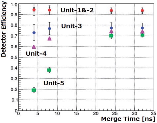
Detector efficiency of Unit-1 to Unit-5 (the data points for Unit-1 and Unit-2 are overlapping) as a function of the hit merge time (see text).
3.2.2. Tracking
The tracking quality is examined from the residual distributions with respect to the tracks reconstructed using the cluster positions of Unit-1 and Unit-3. Here, we require exactly one cluster to be found in each X and Y arrangement in each unit to allow only one track to reconstruct in an event. The time information among the used units is examined to select the tracks coming from the Unit-1 side.
The time profiles shown in Fig. 4 are for typical time differences between Unit-5 and Unit-1, and between Unit-3 and Unit-1 obtained in configuration Layout-1. There are two clusters in the distribution corresponding to the front-arriving (with positive differences) and back-arriving (with negative differences) tracks. The signal cable length of Unit-5 (and Unit-4) was 5 m longer than the others, which shifts the zero of Unit-5 vs. Unit-1 distribution in the positive side. The front-arriving tracks populate more because Unit-1 was more elevated than the others.
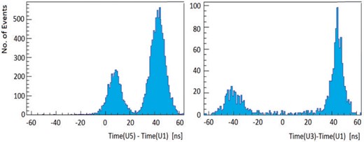
Time differences (left) between Unit-5 and Unit-1, and (right) between Unit-3 and Unit-1. The front-arriving muons are distributed in the larger time-difference peak. Layout-1 configuration.
In evaluating the residual cluster position at Unit-2, for example, both Unit-4 and Unit-5 must record hits within 10 cm to the drawn track (four-fold condition). In addition, the projected track is required to traverse well inside the unit under evaluation, 10 cm inside the fiducial boundary. As shown in Fig. 5, the residuals are well within 5 cm for Unit-2 and 10 cm for Unit-4 and Unit-5, as expected from the scintillator widths of 1 cm for Unit-2 and 4 cm for Unit-4 and Unit-5. In some events, no hit is recorded owing to detector inefficiency.
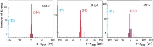
The residuals in the horizontal hit positions evaluated for (left) Unit-2, (middle) Unit-4, and (right) Unit-5. The events with no hit are histogrammed in the leftmost bin.
3.2.3. Unit efficiency—track angle dependence
The detector efficiency as seen in Fig. 5 is studied in more detail. In the reconstruction of the muon track, we take a three-fold condition where three units other than the detector under test are required to record a single cluster in each plane. The track must traverse from the front side. In evaluating the efficiency, the reconstructed tracks are further required to traverse 30 cm inside the fiducial area of the detector under evaluation. Unit-1 to Unit-3 are used as the three units for tracking if none of them is the unit under evaluation. Otherwise, we take Unit-4 or Unit-5 as the third unit.
The detection efficiencies per unit are plotted in Fig. 6 as a function of the track angle |$\alpha $|. Because |$\alpha $| varies with the detector layout on average, the data points are shown for layouts L1–L3 separately. The data with no iron block inserted are analyzed in this evaluation. The efficiency of Unit-1 and Unit-3 systematically decreases as |$\alpha $| approaches zero. The decrease can be attributed to the threshold setting, which was not low enough for these units and sensitive to the variation of the muon path length in the scintillator. The efficiency of Unit-2 remains constant and high. Contrarily, the values for Unit-4 and Unit-5 show larger variations, and the efficiencies are lower on average. The light yield of the 4 cm-wide scintillator bars was apparently smaller than the 1 cm-wide bars, and the threshold could not be set lower with the current DAQ box.
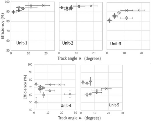
The efficiencies of Unit-1 to Unit-5 shown as a function of track angle |$\alpha$| obtained in (filled circles) Layout-1, (open circles) Layout-2, and (crosses) Layout-3 configurations.
3.2.4. Unit efficiency—dependence on the iron blocks
Because the efficiencies of Unit-4 and Unit-5 are lower than the others, we extended the study to cover other data samples with iron blocks inserted. Figure 7 plots the measured efficiencies of Unit-4 and Unit-5 shown in chorological order. The thicknesses of the iron blocks were changed as shown in the figure. There is no apparent dependence on the iron thicknesses.
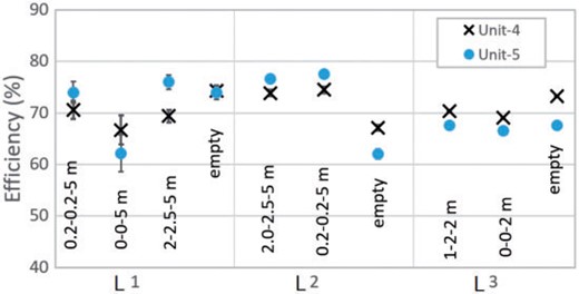
Efficiencies of Unit-4 and Unit-5 plotted in chronological order. Horizontal is the layout number where the iron block thicknesses were changed. The three numbers attached to each data point are iron thicknesses placed between Unit-2 and Unit-4, Unit-4 and Unit-5, and Unit-5 and Unit-3. No iron was placed at “empty.”
3.2.5. Summary of the unit efficiency
The final results for the detector efficiencies are summarized in Table 2. We provide the efficiency of each unit per detector layout considering the |$\alpha $| dependence. For Unit-1 to Unit-3, the rms variation of the efficiency values in Fig. 6 is assigned as the systematic uncertainty. For Unit-4 and Unit-5, the rms variation seen in Fig. 7 is also assigned. As the efficiency is quoted per layout for Unit-4 and Unit-5, we evaluated the upper-side and lower-side systematic uncertainties separately such that the reduced chi-square of the efficiencies measured using subsets of the data samples (layout, track angle, iron thickness) with respect to the weighted mean be unity provided that a common systematics is added to each statistical uncertainty in quadrature.
Detector efficiencies of Unit-1 to Unit-5 shown for detector Layout-1 to Layout-3. The reference tracks are defined using the three units listed as Track. The uncertainties listed in the first rows are statistical and systematic, added in quadrature. The statistical only are in the second rows with the number of tracks given in parentheses.
| Unit | U1 | U2 | U3 | U4 | U5 |
|---|---|---|---|---|---|
| Track | |$U2U3(U4+U5)$| | |$U1U3(U4+U5)$| | |$U1U2(U4+U5)$| | |$U1U2U3$| | |$U1U2U3$| |
| Layout-1 | |$90.6\pm 3.4\%$| | |$94.0\pm 1.5\%$| | |$79.2\pm 5.3\%$| | |${71.7^{+3.6}}_{-2.9}\%$| | |${74.1^{+8.0}}_{-3.5}\%$| |
| |${\pm}\,1.0\%\ (836)$| | |${\pm}\,0.7\%\ (1068)$| | |${\pm}\,1.6\%\ (612)$| | |${\pm}\,1.4\%\ (1477)$| | |${\pm}\,1.8\%\ (912)$| | |
| Layout-2 | |$94.1\pm 3.1\%$| | |$93.9\pm 1.4\%$| | |$85.6\pm 5.1\%$| | |${71.4^{+4.1}}_{-3.3}\%$| | |${73.5^{+9.0}}_{-5.5}\%$| |
| |${\pm}\,0.5\%\ (2240)$| | |${\pm}\,0.5\%\ (2637)$| | |${\pm}\,2.4\%\ (1301)$| | |${\pm}\,0.6\%\ (6983)$| | |${\pm}\,4.5\%\ (2330)$| | |
| Layout-3 | |$96.2\pm 3.0\%$| | |$96.1\pm 1.4\%$| | |$91.3\pm 5.0\%$| | |${71.2^{+3.6}}_{-2.9}\%$| | |${67.1^{+7.8}}_{-3.1}\%$| |
| |${\pm}\,0.1\%\ (27735)$| | |${\pm}\,0.1\%\ (36686)$| | |${\pm}\,0.2\%\ (19788)$| | |${\pm}\,1.4\%\ (74243)$| | |${\pm}\,0.4\%\ (31206)$| |
3.3. Efficiency of single-cluster requirement
The inefficiency due to the single-cluster requirement was evaluated from the data. The single-cluster requirement was first dropped for Unit-1, and then subsequent tracking was performed for all cluster combinations. For the event satisfying the standard tracking criteria, the cluster multiplicity in Unit-1 was examined. Because the tracking was performed using Unit-2 and one of Unit-3 to Unit-5 in addition, the fraction of multiple clusters was derived separately for each of Unit-3 to Unit-5 and per Layout-1 to Layout-3. This study was repeated for Unit-2. The results were combined to evaluate the overall correction factor and its uncertainty. For the case using (Unit-3, Unit-4, Unit-5) for the third plane, the correction factors due to the single-cluster requirement are (1.04–1.06, 1.09–1.15, 1.15–1.18), with uncertainty better than 1%.
3.4. Detector acceptance
The acceptance sum of |$\sum {dSd\Omega } $| for the detector system is shown in Fig. 8 as a function of the track angle |$\alpha $|. Here, the combinations giving the same tan |$\alpha $| value are summed over with a binning size of 0.01. The curves are characterized by the layout and the third unit that is used in addition to Unit-1 and Unit-2 to reconstruct the tracks.
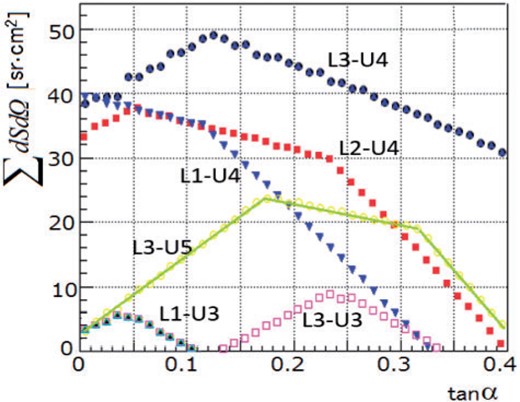
The acceptance of the detector system as a function of the tangent of the track angle |$\alpha $|. The labels of the curves denote the three layouts (L1–L3) and the third unit used for tracking in addition to Unit-1 and Unit-2. Some other curves covering intermediate regions are not plotted.
The data taken in Layout-1 and Layout-2 are merged to cover the region |$0.0<\tan \alpha <0.11$| with the requirement of Unit-3 acceptance and for a maximal iron thickness of 9.5 m. Because Unit-3 was placed closer in Layout-3, the acceptance (L3-U3) covers a larger |$\tan \alpha $| range, covering |$0.14<\tan \alpha <0.34$|, whereas the iron block allowed 5 m in this layout. In comparing the data with Ref. [2], the coverage was further extended up to |$\tan \alpha <0.40$| using the L3-U5 acceptance but for a maximal iron thickness of 3 m.
3.5. Number of events
The event selection is summarized as follows:
(1) Only one hit cluster is found in each X–Y plane of Unit-1 and Unit-2. The hit merge time and the number of consecutive hits in the cluster definition are the same as described in Sect. 3.2, 24 ns and a maximum of three, respectively.
(2) The track extrapolated from Unit-1 and Unit-2 traverses the Unit-3 area 10 cm inside the boundary. This was not required in comparison with Ref. [2] in Sect. 4.2.
(3) Require a hit in the third unit (Unit-3, Unit-4, or Unit-5) under consideration. The hit is found in the specified time window: |$T$|(Unit-3) |$- T$|(Unit-1) > 0 and |$T$|(Unit-3) |$- T$|(Unit-2) > 0 for Unit-3; |$T$|(Unit) |$- T$|(Unit-1) > 20 ns and |$T$|(Unit) |$- T$|(Unit-2) > 20 ns for Unit|$=$| Unit-4 or Unit-5.
The above requirements are applied to extract the momentum dependence of the muon flux. Figure 9 shows the time correlations obtained in Layout-2 and Layout-3 concerning requirement (3). The tracks coming from the Unit-1 side are well separated from the backward tracks.
![Correlations of time differences between the third Unit (Unit-3, Unit-4, or Unit-5) with respect to Unit-1 (horizontal axis) and Unit-2 (vertical axis) in Layout-2 [a), b), c)] and in Layout-3 [d), e), f)]. The number of events is shown along the third axis.](https://oup.silverchair-cdn.com/oup/backfile/Content_public/Journal/ptep/2017/12/10.1093_ptep_ptx164/4/m_ptx164f9.jpeg?Expires=1750204179&Signature=IUur3TiBwSHvQfnYuwUQAAB~fV2ryH9gjoIjT1~7GmZuop9XW-DJ8OOfch8PEX39AV3-CeE2Co0piqHkt6cZEPQZGtToY1yWJL2hm2Ik0XCPdSOM9BlCreVWhkIBadHSa-Vmef0uknIRFFPqj3mYFrYJRdDj-982kXGcMVbGk0SACPgZc7IKzIiwgTwL3MaDJVapfRcrkyfmZNXpJ0Xk7U5tycWhw5JdrnGI6lmVBQibF298dBwsHAUuKQMGH-QbISkWTk4vINsmbdcpgDHG0ahDjIwsU1f7lxpnA0WoNCjVrVJZfcdB36KIjBwsN20ElkUt~~aWyvGHr~nfLpPnmg__&Key-Pair-Id=APKAIE5G5CRDK6RD3PGA)
Correlations of time differences between the third Unit (Unit-3, Unit-4, or Unit-5) with respect to Unit-1 (horizontal axis) and Unit-2 (vertical axis) in Layout-2 [a), b), c)] and in Layout-3 [d), e), f)]. The number of events is shown along the third axis.
Fig. 9 Correlations of time differences between the third Unit (Unit-3, Unit-4, or Unit-5) with respect to Unit-1 (horizontal axis) and Unit-2 (vertical axis) in Layout-2 [a), b), c)] and in Layout-3 [d), e), f)]. The number of events is shown along the third axis.
3.6. Systematic uncertainty
The main source of systematic uncertainty is the unit efficiency evaluation. The evaluation procedure is described in Sect. 3.2, and the results are summarized in Table 2. The event selection including the requirements for the merge time, single-cluster requirement per X–Y plane, and time difference selection has a secondary effect. The uncertainties in the merge time and time cut were evaluated from the distribution tails.
3.7. Muon range
The muon momentum thresholds are calculated from the muon range [9] in the iron block. Typical values we calculated are summarized in Table 3. In corresponding the iron thickness and the momentum threshold, the average iron thickness as dependent on the track angle was used.
Summary of muon threshold momentum |$P_{\it cut}$| for the corresponding iron thickness.
| Thickness | R/M (g cm|$^{-2}$| GeV|$^{-1}$|) | |$\beta\gamma$| | |$P_{\textit{cut}}$| (GeV/c) |
|---|---|---|---|
| 0 | 0.02 | ||
| 20 cm | 1326 | 3.4 | 0.37 |
| 40 cm | 2652 | 5.5 | 0.58 |
| 200 cm | 1.33 |$\times$| 104 | 25 | 2.64 |
| 450 cm | 2.98 |$\times$| 104 | 52 | 5.49 |
| 950 cm | 6.29 |$\times$| 104 | 110 | 11.6 |
4. Results
4.1. Muon flux dependence on the zenith angle with no iron
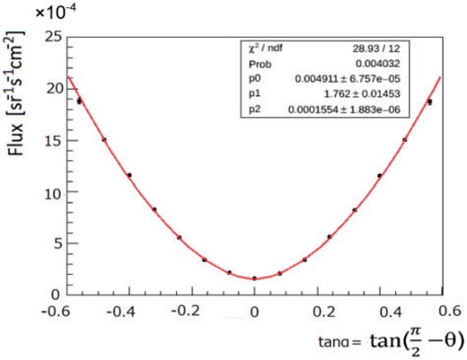
Muon flux as a function of elevation angle |$ \alpha$| measured using Unit-1 and Unit-2 only. No iron inserted. The curve is fitted with a simple function as described in the text.
Here the data points for negative |$\tan \alpha $| represent the tracks coming from the backside.
4.2. Muon flux in |$\theta =75\pm 7^{\circ}$|, comparison with DEIS
The muon data obtained in the Layout-2 and Layout-3 configurations are compared with the existing muon flux data (DEIS group [2]). In Ref. [2], the flux values integrated over the zenith angle range of |$\theta =75\pm 7^{\circ}(0.14<\tan \ \alpha <0.40)$| are available as a function of the muon momentum threshold.
In Fig. 11, the obtained flux values relevant in this comparison are shown as a function of |$\alpha $| for different iron thicknesses. Because the coverage in some configurations does not extend fully to |$0.14<\tan \ \alpha <0.40$|, the coverage for 5 m-thick iron being limited to |$0.14<\tan \ \alpha <0.34$| for example, we apply a correction factor to account for this deficit. The flux values estimated in the DEIS range |$0.14<\tan \ \alpha <0.40$| derived from the values measured in |$0.14<\tan \ \alpha <0.34$| are listed in Table 4. The correction factor to account for the acceptance deficit is derived from the DEIS fitting result (Eq. (2) of Ref. [2]). The factor is barely dependent on the muon momentum threshold, and we take the factor 1.35 to be multiplied by the flux integrated over |$0.14<\tan \alpha <0.34$|. Also listed in Table 4 are some of the flux values measured withdrawing the requirement of Unit-3 in the acceptance to cover the |$0.14<\tan \ \alpha <0.40$| range. We found a systematic difference of approximately 10%, which is added in quadrature for those values to which is applied the 1.35 correction factor. Figure 11 compares the flux data in |$0.14<\tan \ \alpha <0.40$| with [2]. The two sets of values are in fairly good agreement.
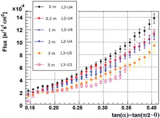
Muon flux as a function of tan |$\alpha $| for different iron thicknesses used for comparison with the DEIS data. The iron thickness, layout number, and the third unit in the flux calculation are shown in the legend.
Muon flux integrated over |$68^{\circ}<\theta<82^{\circ}$| is calculated for different iron thicknesses with the corresponding momentum thresholds calculated from Table 3 considering the track angle |$\alpha$|. The fifth column lists the flux values measured in the range |$0.14<\text{tan} \ \alpha<0.34$| and multiplied by a factor of 1.35 (see text) to normalize the measured values to the flux in |$68^{\circ}<\theta<82^{\circ}$| (|$0.14<\text{tan} \ \alpha<0.40$|). The last column lists the flux measured directly in the region |$0.14<\text{tan} \ \alpha<0.40$|.
| Iron thickness | |$P_{\it cut}$| (GeV/c) | Layout-3rd Unit | Number of Events | Flux [sr|$^{-1}$| s|$^{-1}$| cm|$^{-2}$|] in |$68^{\circ}<\theta<82^{\circ}$| from |$0.14<\text{tan} \ \alpha<0.34$| | Flux [sr|$^{-1}$| s|$^{-1}$| cm|$^{-2}$|] |$0.14<\text{tan} \ \alpha<0.40$| |
|---|---|---|---|---|---|
| 0 | 0.02 | L3-U4 | 615,103 | |${5.63^{+0.30}}_{-0.35} \times 10^{-4}$| | |${6.36^{+0.34}}_{-0.39} \times 10^{-4}$| |
| 20 cm | 0.38 | L2-U4 | 111,511 | |${5.02^{+0.25}}_{-0.28} \times 10^{-4}$| | |
| 100 cm | 1.44 | L3-U4 | 169,161 | |${4.54^{+0.25}}_{-0.28} \times 10^{-4}$| | |${5.15^{+0.28}}_{-0.32} \times 10^{-4}$| |
| 200 cm | 2.73 | L2-U4 | 87,573 | |${4.46^{+0.25}}_{-0.29} \times 10^{-4}$| | |
| 300 cm | 4.00 | L3-U5 | 124,980 | |${3.68^{+0.22}}_{-0.45} \times 10^{-4}$| | |${4.14^{+0.25}}_{-0.50} \times 10^{-4}$| |
| 500 cm | 6.49 | L3-U3 | 22,197 | |${3.16^{+0.24}}_{-0.24} \times 10^{-4}$| |
We should note here that the present measurement based on muon range resulted in a similar muon flux value to the previous result obtained using a magnetic spectrometer, whereas more careful control of systematics is necessary in the present case due mainly to changes in the setup rendering it more sensitive to systematic uncertainties.
4.3. Muon flux in horizontal region |$0<\tan \ \alpha <0.11$|
The horizontal muon flux in |$0< \tan \ \alpha <0.11$| is measured similarly. The integrated flux values are summarized in Table 5 and plotted in Fig. 12 as a function of the momentum threshold. We notice that the integrated flux is almost flat in the forward region, meaning that the muons with lower momenta are less frequent.
![Integrated muon flux as a function of the momentum threshold. The data of Ref. [2] are compared with this work in the range $0.14< \text{tan} \ \alpha<0.40$. The data in the horizontal region $0< \text{tan} \ \alpha<0.11$ are also plotted.](https://oup.silverchair-cdn.com/oup/backfile/Content_public/Journal/ptep/2017/12/10.1093_ptep_ptx164/4/m_ptx164f12.jpeg?Expires=1750204179&Signature=x2mennmeO1vb3GAvUTPl1AoM~AZ4seZP6zdtCFmptO4oyUyrohxdvmlAqyzPxqRZj1yfEUAKKTj9CmIhpzIXHkIDGn5owc6vealJ2lv1E6tKytpdI-ZhSMRR06punUpLV-N3f8XqiT-TP2zTEY8pzNY1vNgyUniiyzDeDfzknFOQbPFVvETHi86IVQS2ZZKP43e2PcAQ6jvdkeN6-fb4bKwJXwDMephcOgEU~bBIwr4xoIeuKYUvAletj-AKe-NX8qw2FjctSFMhIME1pTDfUatplk3LYPJKXQ08aJ~r6i3wYeeLlHbaPxzCt6RwpmLF60v5TRW9isQEk6GkxokJGA__&Key-Pair-Id=APKAIE5G5CRDK6RD3PGA)
Integrated muon flux as a function of the momentum threshold. The data of Ref. [2] are compared with this work in the range |$0.14< \text{tan} \ \alpha<0.40$|. The data in the horizontal region |$0< \text{tan} \ \alpha<0.11$| are also plotted.
Muon flux integrated over |$0<\text{tan} \ \alpha<0.11$| for different iron thicknesses. The mean momentum threshold |$P_{\it cut}$| is calculated from Table 2 considering the track angle.
| Iron Thickness | |$P_{\it cut}$| (GeV/c) | Layout-3rd Unit | Number of Events | Flux [sr|$^{-1}$| s|$^{-1}$| cm|$^{-2}$|] |$0<\text{tan} \ \alpha<0.1$| |
|---|---|---|---|---|
| 0 | 0.02 | L1-U3 | 812 | |${4.64^{+0.69}}_{-0.69} \times 10^{-5}$| |
| 20 cm | 0.36 | L2-U4 | 12,324 | |${4.15^{+0.29}}_{-0.31} \times 10^{-5}$| |
| 40 cm | 0.58 | L2-U5 | 5,388 | |${3.80^{+0.25}}_{-0.52} \times 10^{-5}$| |
| 100 cm | 1.39 | L3-U4 | 11,057 | |${3.98^{+0.25}}_{-0.28} \times 10^{-5}$| |
| 200 cm | 2.64 | L2-U4 | 15,965 | |${3.68^{+0.25}}_{-0.27} \times 10^{-5}$| |
| 300 cm | 3.86 | L3-U5 | 2,431 | |${3.33^{+0.34}}_{-0.50} \times 10^{-5}$| |
| 500 cm | 6.10 | L1-U3 | 196 | |${4.0^{+1.0}}_{-1.0} \times 10^{-5}$| |
| 540 cm | 6.58 | L1-U3 | 513 | |${4.17^{+0.70}}_{-0.70} \times 10^{-5}$| |
4.4. Empirical expression for the muon flux

The obtained parameters are summarized in Table 6. Because the systematic uncertainty is large, the resulting uncertainties of the parameters are huge. However, the central values of the measured flux are well reproduced by the parametrized functions. The fit deviations are also listed in Table 6, where “relative” refers to the rms spread of the deviations (flux measured and calculated) divided by the measured value, and “normalized” refers to the rms spread of the deviations divided by the uncertainty of the measured value. All relative deviations are within 40% in both regions. The overall uncertainty of the fit is well below the measured uncertainty in the |$0.14< \tan \ \alpha <0.40$| region, and consistent with the uncertainty in the |$0< \tan \ \alpha <0.11$| region.
Results of parameter fitting to reproduce the integrated muon flux in the tan |$\alpha $| regions as listed. The threshold momentum is up to 6.1 GeV/c in |$0.14< \tan \ \alpha<0.34$| and 3.9 GeV/c in |$0.34< \tan \ \alpha<0.40$| (same parameters are applicable), and 11.6 GeV/c in |$0< \tan \ \alpha<0.11$|.
| Parameters | |$P_{\mathrm{cut}}$||${<}$| 6.1 GeV/c in |$0.14< \tan \ \alpha<0.34$| | |
|---|---|---|
| applicable range | |$P_{\mathrm{cut}}$||${<}$| 3.9 GeV/c in |$0.34< \tan \ \alpha<0.40$| | |$P_{\mathrm{cut}}$||${<}$| 11.6 GeV/c in |$0< \tan \ \alpha<0.11$| |
| |$p$| [sr|$^{\mathrm{-1\thinspace }}$|s|$^{\mathrm{-1\thinspace }}$|cm|$^{\mathrm{-2}}$|] | (2.29 |$\pm$| 15.74) |$\times$| 10|$^{\mathrm{-5}}$| | (6.32 |$\pm$| 0.49) |$\times$| 10|$^{\mathrm{-6}}$| |
| |$q$| [sr|$^{\mathrm{-1\thinspace }}$|s|$^{\mathrm{-1\thinspace }}$|cm|$^{\mathrm{-2}}$|] | (4.4 |$\pm$| 3.6) |$\times$| 10|$^{\mathrm{-4}}$| | (1.60 |$\pm$| 0.19) |$\times$| 10|$^{\mathrm{-3}}$| |
| |$m$| | 1.80 |$\pm$| 0.93 | 1.33 |$\pm$| 0.05 |
| |$r$| | 0.03 |$\pm$| 0.20 | (2.7 |$\pm$| 3.8) |$\times$| 10|$^{\mathrm{-2}}$| |
| |$s$| | 0.11 |$\pm$| 0.39 | (–1. |$\pm$| 1.3) |$\times$| 10|$^{\mathrm{-2}}$| |
| Fit deviations | Relative: 26% | Relative: 14% |
| Normalized: 0.28 | Normalized: 1.26 | |
| 182 data points | 77 data points |
5. Summary
The cosmic muon flux in the zenith angle range 0 |${<}$| cos |$\theta $||${<}$| 0.37 has been measured using a muon range detector comprising scintillator hodoscope systems with cross-section of 1 m |$\times$| 1 m or larger. The inserted iron blocks of up to 9.5 m for the |${<}$| cos |$\theta $||${<}$| 0.12 range, up to 5.0 m for the 0.14 |${<}$| cos |$\theta $||${<}$| 0.32 range, and up to 3 m for the 0.32 |${<}$| cos |$\theta $||${<}$| 0.37 range correspond to the momentum thresholds of up to 11.6 GeV/c, 6.1 GeV/c, and 3.9 GeV/c, respectively. The present data are in agreement with the previous measurement by the DEIS group for 0.14 |${<}$| cos |$\theta $||${<}$| 0.37, and extended to lower zenith angle ranges. The new set of data covering the lower zenith angle range is extremely useful for muon radiography to investigate the inner status of, e.g., nuclear plants.
Acknowledgments
The present study has been carried out as a project supported by the International Research Institute for Nuclear Decommissioning IRID. We appreciate the understanding and warm support provided by KEK Director in General, Prof. M. Yamauchi.
References
Author notes
Present address: Japan Atomic Energy Agency
Present address: Iwate Prefectural University
Present address: Toshiba Co., Ltd.
