Excitation energy spectra of the |$\Lambda_{c}$| and |$\Lambda_{b}$| baryons in a finite-size diquark model

Abstract

The excitation energies of the |$\Lambda_{c}$| and |$\Lambda_{b}$| baryons are investigated in a finite-size diquark potential model, in which the heavy baryons are treated as bound states of a charm quark and a scalar–isoscalar diquark. The diquark is considered as a sizable object. The quark–diquark interaction is calculated as a sum of the quark–quark interaction that is assumed to be half of the quark–antiquark interaction for the color singlet. The potential parameters in the quark–antiquark interaction are fixed so as to reproduce the charmonium spectrum. We find the diquark size to be 1.1 fm for the diquark mass 0.5 GeV/|$c^{2}$| to reproduce the |$1p$| excitation energy of |$\Lambda_{c}$|⁠. In this model, the |$\Lambda_{c}$| and |$\Lambda_{b}$| excitation spectra are reproduced well, while this model does not explain |$\Lambda_{c}(2765)$|⁠, whose isospin and spin–parity are still unknown. Thus, the detailed properties of |$\Lambda_{c}(2765)$| are very important to the presence of the diquark in heavy baryons as an effective constituent. We also discuss the |$\Xi_{c}$| spectrum with the scalar strange diquark.

1. Introduction

Understanding hadron spectroscopy in terms of quark–gluon dynamics is one of the challenging issues in hadron physics. In particular, finding effective elements of the hadron is important for intuitive understanding of the hadron structure and excitation modes. The constituent quark is one of the successful ideas explaining the hadron structure. For instance, the anomalous magnetic moments of the nucleon and its flavor partners can be calculated as the matrix element of the quark magnetic moment operator in terms of the baryonic state constructed by the spin–flavor configuration of quarks, being reproduced well if one regards the constituents as a point-like Dirac fermion with a mass being one-third of the nucleon. It is interesting that, although the dynamics inside the hadron is very complicated, such a simple picture works. This may be because the constituent quark can be an effective degree of freedom for the hadron structure as a quasiparticle formed as a consequence of the complicated field-theoretical dynamics of quarks and gluons. The low-lying excitation spectra of heavy quarkonia are also explained by the excitation of the constituent quarks in a simple confinement potential, the so-called linear-plus-Coulomb-type potential. The diquark, which is a pair of two quarks, is a longstanding strong candidate of a constituent of a hadron [1-3]. The diquark is regarded as a particle-like object in this study. Having color charge, the diquark cannot exist alone in vacuum. So far, the existence of diquark correlation inside hadrons has been indicated by phenomenological findings in baryon spectroscopy, weak non-leptonic decays, parton distribution functions, and fragmentation functions. In particular, one expects the existence of the scalar diquark with flavor, spin, and color antisymmetric configuration, the so-called good diquark, thanks to the most attractive correlation in perturbative quantum chromodynamics (QCD) and instanton-induced interaction [4]. The strong correlation in the scalar diquark has been observed in lattice calculations [5-8].

In order to investigate the presence of the strong diquark correlation in the hadron phenomenologically, we focus on the excited spectra of heavy baryons. So far, many studies have been done on baryon spectra in terms of quark–diquark models. The mass spectra of the |$\ell = 1$| and |$\ell=2$| excited states of non-strange baryons were studied based on a diquark–quark model [9] by using the SU(6)|$\otimes$|O(3) classification [10] and focusing on the fine structure by spin–orbit interactions. In a relativistic formulation [11], the ground states of spin-3/2 baryons were investigated. The radial and orbital excitations of baryons were calculated in a diquark–quark model with a confinement potential reproducing meson spectra [12], and there detailed analyses for light flavor baryon spectra were given. The mass spectra of the excited heavy baryons with one heavy quark were studied in a relativistic quark–diquark model in which diquark bound states were solved relativistically and the inner structure of the diquark was taken into account [13,14]. A finite size for the diquark has been suggested in Refs. [8,15], and there the size can be as large as 1 fm. Reference [16] tested the heavy quark–light diquark approximation for baryons and found that it works reasonably well but with a large diquark size. The newly observed |$\Omega_{c}$| states were investigated in a strange diquark model [17]. In Ref. [18], the ground state masses of |$\Lambda$|⁠, |$\Lambda_{c}$|⁠, and |$\Lambda_{b}$| were calculated in a diquark QCD sum rule, in which the scalar |$ud$| diquark is explicitly considered as a fundamental field in the operator product expansion. The QCD sum rule successfully reproduced the observed |$\Lambda$|’s masses with a “constituent” diquark mass of 0.4 GeV, having satisfied the standard criteria for the QCD sum rule to work.

Baryons composed of one heavy quark and two light quarks are good systems in which to study the diquark correlation. As reported in Refs. [19,20], the quark–antiquark configurations dominate in meson wavefunctions, and the diquark components are rather suppressed, because the diquark correlation is weaker than the quark–antiquark correlation. Thus, once the antiquark is present close to the diquark, the diquark may be easily broken up and form a quark–antiquark pair. In light baryons, the diquark correlation may be important for their structure, but rearrangement of the diquark with the remaining quark can also be important due to the symmetry among light quarks.

In our previous work [21], we have investigated excited spectra of the |$\Lambda_{c}$| and |$\Lambda_{b}$| baryons in a quark–diquark model in order to examine the possible existence of a diquark inside a baryon based on phenomenological facts. In this model, the |$ud$| diquark is treated as a point-like particle with isospin 0 and spin 0, and the heavy quark and the diquark are bound in the linear-plus-Coulomb-type potential. It has been found that, if one uses the potential parameters that reproduce the charmonium spectrum, one obtains a much greater |$1p$| excitation energy for |$\Lambda_{c}$| than in the observation, and in order to reproduce the observed excitation energy, one has to reduce the string tension by half even though the antiquark and diquark have the same color charge. It has also been reported that the size effect of the diquark could solve this problem.

In this paper, we consider the size of the diquark and calculate the excitation energy of |$\Lambda_{c}$| and |$\Lambda_{b}$| by treating the diquark as a rigid rotor, in order to examine whether the size effect can explain the excitation spectra of the heavy baryons. The quark–diquark interaction is calculated as a convolution of the quark–quark interaction. We will see that the finite-size effect reduces the quark–diquark interaction at short distances. This makes the excitation energies smaller for higher partial waves. We will find that the diquark size |$\rho \simeq 1.1$| fm reproduces the observed excitation energy of the |$1p$||$\Lambda_{c}$| state, and with this size the |$\Lambda_{c}$| and |$\Lambda_{b}$| spectra are well reproduced. We also discuss the mass and size of the strange diquark from the |$\Xi_{c}$| mass spectrum.

2. Formulation

We take a diquark–quark model for the heavy baryon that is composed of one heavy quark (⁠|$c$| or |$b$| quark) and two light quarks. In the diquark–quark model, assuming that two light quarks forms a scalar diquark with antisymmetric flavor configuration, which is the so-called good diquark, we calculate the spectrum of the heavy baryon as a two-body problem with a heavy quark and a diquark. In the present work, we consider the diquark to be a sizable object, not a point particle, and treat the diquark as a rigid rotor with the moment of inertia |$I=\rho^{2} m_{d}/4$|⁠, where |$\rho$| is the size of the diquark (the distance between two light quarks) and |$m_{d}$| is the diquark mass. The distance between the light quarks, |$\rho$|⁠, is no longer a dynamical variable.

In the center-of-mass system, the coordinate representation of the Hamiltonian operator for the heavy quark and diquark system is written by

\begin{equation}\label{eq:H} H = m_{h} + m_{d} - \frac{\hbar^{2}}{2\mu}\frac{1}{r} \frac{d^{2}}{dr^{2}}r + \frac{ L_{\lambda}^{2}}{2\mu r^{2}} + V(\vec r, \hat \rho) + \frac{ L_{\rho}^{2}}{2I}, \end{equation}

(1)

where |$m_{h}$| and |$m_{d}$| are the masses of the heavy quark and the diquark, respectively, |$\mu$| is the reduced mass of the diquark and the heavy quark, |$r$| and |$ L_{\lambda}$| are the radius and the angular momentum of the relative coordinate, |$\hat L_{\rho}$| is the angular momentum of the diquark, and |$V(\vec r, \hat \rho)$| represents the interaction between the diquark and the heavy quark that depends on the relative coordinate |$\vec r$| and the orientation of the diquark |$\hat \rho$|⁠.

In the present work, the interaction is given by the sum of the interactions between the heavy quark and the light quarks inside the diquark as

\begin{equation} V(\vec r, \hat \rho) = V_{qq}(\vec r - \vec \rho/2) + V_{qq}(\vec r + \vec \rho /2) \label{dqpot} \end{equation}

(2)

with |$\vec \rho = \rho \hat \rho$| and the quark–quark interaction |$V_{qq}$| for the |$\bar {\boldsymbol 3}$| color configuration. We presume that the strength of the |$\bar {\boldsymbol 3}$| interquark interaction |$V_{qq}$| is half of the color electric quark–antiquark interaction |$V_{\bar qq}$| for the color singlet configuration, |$V_{qq} = \frac12 V_{\bar qq}$|⁠, which is the case for the one-gluon exchange calculation. The quark and antiquark interaction is assumed to be spherical and given by a Coulomb-plus-linear form [22,23]

\begin{equation} V_{\bar qq}(r) = - \frac{4}{3} \frac{\alpha}{r} \hbar c + k r + V_{0} \label{pot} \end{equation}

(3)

with three parameters, |$\alpha$|⁠, |$k$|⁠, and |$V_{0}$|⁠. The parameter |$V_{0}$| adjusts the absolute value of the mass spectrum and is irrelevant in this work, because we are interested in the excitation energies measured from the ground state. A choice of parameters, |$\alpha = 0.4$| and |$k=0.9$| GeV fm|$^{-1}$|⁠, works well to produce the charmonium and bottomonium spectra [21,24]. It is also reported in Ref. [21] that the calculation of the first excitation energies of the |$D$|⁠, |$D_{s}$|⁠, |$B$|⁠, and |$B_{s}$| mesons with these values for the parameters is consistent with the experimental observation. According to these phenomenological successes in reproducing the meson spectra, we use the following values:

\begin{equation} \alpha = 0.4, \qquad k= 0.9\ {\rm GeV/fm} \end{equation}

(4)

for the potential parameters. In this study, because we are interested in the global structure of the baryon spectrum in the quark–diquark model, we do not take into account fine-structure interactions, such as spin–orbit interaction, for the present. Because we do not consider spin-dependent forces, the angular momentum of the system, |$L$|⁠, is a good quantum number to label the states. (For the spinless diquark, the total angular momentum of the system |$J$| is given by |$J=L\pm \frac{1}{2}$|⁠, and these states are degenerate due to the lack of the spin–orbit interaction).

Now let us decompose the quantum state of the quark–diquark system |$|\Psi \rangle$| in terms of the angular momentum |$L$|⁠:

\begin{equation} | \Psi \rangle = |S \rangle + |P \rangle + | D \rangle + \cdots. \end{equation}

(5)

Each angular momentum state |$|L\rangle$| is written by a combination of the angular momentum states of the relative coordinate and the diquark, which we write as |$|\ell_{\rho}, \ell_{\lambda} \rangle_{L} $| with the diquark angular momentum |$\ell_{\rho}$| and the relative angular momentum |$\ell_{\lambda}$|⁠. Because we consider a scalar diquark with asymmetry flavor configuration, symmetry only allows the diquark angular momentum |$\ell_{\rho}$| to be an even number. Thus, the low angular momentum states are given as

\begin{eqnarray} |S \rangle &=& |0,0\rangle_{S} + | 2,2 \rangle_{S} + \cdots, \end{eqnarray}

(6)

\begin{eqnarray} |P \rangle &=& |0,1\rangle_{P} + | 2,1 \rangle_{P} + | 2,2 \rangle_{P} + \cdots, \end{eqnarray}

(7)

\begin{eqnarray} |D \rangle &=& |0,2\rangle_{D} + | 2,0 \rangle_{D} + | 2,1 \rangle_{D} + |2,2\rangle_{D} + \cdots. \end{eqnarray}

(8)

The construction of the states is explained in Appendix A.

We solve the eigenequation |$\hat H | L \rangle = M | L \rangle$| for each angular momentum state to obtain the baryon mass |$M$| as a bound state of the heavy quark and diquark. For this purpose we calculate the matrix element |$_{L}\langle \ell_{\rho}^{\prime}, \ell_{\lambda}^{\prime} | \hat H | \ell_{\rho}, \ell_{\lambda}\rangle_{L}$| for each partial wave |$L$| and diagonalize the Hamiltonian. As we shall see later, it will turn out that the off-diagonal elements are negligibly small and the diagonalization plays a minor role. Because the state |$ | \ell_{\rho}, \ell_{\lambda}\rangle_{L}$| has definite angular momenta of the diquark and the relative motion, it is an eigenstate of |$\hat L^{2}_{\rho}$| and |$\hat L^{2}_{\lambda}$|⁠:

\begin{equation} \hat L^{2}_{\rho} | \ell_{\rho}, \ell_{\lambda}\rangle_{L} = \ell_{\rho}(\ell_{\rho}+1) \hbar^{2} | \ell_{\rho}, \ell_{\lambda}\rangle_{L}, \qquad \hat L^{2}_{\lambda} | \ell_{\rho}, \ell_{\lambda}\rangle_{L} = \ell_{\lambda}(\ell_{\lambda}+1) \hbar^{2} | \ell_{\rho}, \ell_{\lambda}\rangle_{L}. \end{equation}

(9)

Now writing the radial wavefunction as |$R(r)$| and using the orthogonality of the angular moment eigenstates, we obtain the matrix elements as

\begin{eqnarray} && {}_{L}\langle \ell_{\rho}, \ell_{\lambda} | \hat H | \ell_{\rho}, \ell_{\lambda}\rangle_{L} = m_{h} + m_{d}\nonumber \\ &&\quad{} + \int r^{2} dr R^{*}(r) \left[ - \frac{\hbar^{2}}{2\mu} \frac{1}{r} \frac{d^{2}}{dr^{2}} r + \frac{\ell_{\lambda}(\ell_{\lambda}+1)\hbar^{2}}{2\mu r^{2}} + V_{\rm eff}(r) + \frac{\ell_{\rho}(\ell_{\rho}+1)\hbar^{2}}{2I} \right] R(r) \label{MEdiag} \end{eqnarray}

(10)

for the diagonal elements and

\begin{equation} _{L}\langle \ell_{\rho}^{\prime}, \ell_{\lambda}^{\prime} | \hat H | \ell_{\rho}, \ell_{\lambda}\rangle_{L} = \int r^{2} dr R^{*}(r) V_{\rm eff}(r) R(r) \label{MEoff} \end{equation}

(11)

for the off-diagonal elements. Here we have introduced the effective potential for the radial motion |$V_{\rm eff}(r)$| that depends on |$L$|⁠, |$\ell_{\rho}$|⁠, and |$\ell_{\lambda}$|⁠. The effective potential |$V_{\rm eff}(r)$| is calculated by integrating the quark–diquark interaction potential (2) with respect to the solid angle integrals of the relative coordinate |$\Omega_{r}$| and the diquark orientation |$\Omega_{\rho}$|⁠:

\begin{eqnarray} V_{\rm eff}(r; L, \ell_{\rho}, \ell_{\lambda}) &=&\ _{L}\langle \ell_{\rho}^{\prime}, \ell_{\lambda}^{\prime} | V(\vec r, \hat \rho) | \ell_{\rho}, \ell_{\lambda}\rangle_{L} \end{eqnarray}

(12)

\begin{eqnarray} &=& \int d\Omega_{r} d\Omega_{\rho} \left[ Y_{\ell_{\rho}^{\prime}}^{*m_{\rho}^{\prime}}(\Omega_{\rho}) Y_{\ell_{\lambda}^{\prime}}^{*m_{\lambda}^{\prime}}(\Omega_{r}) \right]_{L} V(\vec r, \hat \rho) \left[Y_{\ell_{\rho}}^{m_{\rho}}(\Omega_{\rho}) Y_{\ell_{\lambda}}^{m_{\lambda}}(\Omega_{r}) \right]_{L}, \label{eq:Veff} \end{eqnarray}

(13)

where |$[\cdots]_{L}$| means that one should take the appropriate linear combination so as to make the combined angular momentum |$L$|⁠. The explicit expression for each matrix element is given in Appendix B. We numerically solve the radial Schrödinger equation,

\begin{equation}\label{Sheq} \left[- \frac{\hbar^{2}}{2\mu} \frac{d^{2}}{dr^{2}} + \frac{\ell_{\lambda}(\ell_{\lambda}+1)\hbar^{2}}{2\mu r^{2}} + V_{\rm eff}(r) + \frac{\ell_{\rho}(\ell_{\rho}+1)\hbar^{2}}{2I} \right] \chi(r) = E \chi(r), \end{equation}

(14)

with |$R(r) = \chi(r) / r$|⁠, and obtain the diagonal matrix element as |$m_{h}+m_{d} +E$|⁠. For the off-diagonal elements, we perform the integral (11) using the wavefunctions that are obtained from the Schrödinger equation for the diagonal components.

3. Results

In this section, we show the numerical results of our calculation. First we show the effective potential of the diquark–quark interaction for several diquark sizes. Here we see that the size of the diquark reduces the interaction strength at shorter distances. Then, we present our results on the excitation energy spectrum of |$\Lambda_{c}$| obtained by solving the radial Schrödinger equation (14) as a function of the diquark size |$\rho$|⁠. There we determine the diquark size so as to reproduce the excitation energy of |$\Lambda_{c}$| with |$L =1$| for the diquark mass |$0.5$| GeV/|$c^{2}$|⁠. Next we show the calculated energy spectra of |$\Lambda_{c}$| and |$\Lambda_{b}$| using the determined diquark size and compare them with the experimental observation. Then, we investigate the diquark mass dependence of the diquark size that reproduces the |$p$|-wave excitation energy. Finally we calculate the |$\Xi_{c}$| mass spectrum with the strange diquark |$qs$| and determine the strange diquark mass and size. In our calculation, the masses of the charm quark and the bottom quark are fixed at |$1.5$| GeV/|$c^{2}$| and 4.0 GeV/|$c^{2}$|⁠, and we use |$\alpha=0.4$| and |$k=0.9$| GeV/fm for the potential parameter that reproduces the charmonium spectrum well. We have checked that the qualitative feature of our results is insensitive to the fine-tuning of these parameters.

3.1. Effective potential between diquark and heavy quark

First of all, we discuss the interaction potential between the heavy quark and the sizable diquark. The definition of the effective potential of the quark–diquark interaction is given in Eq. (13) and the explicit calculation is done in Appendix B. We are interested in the lower excitation spectrum. Here we show the effective potentials for the lower energy states. In Fig. 1, we plot the effective potentials with several sizes of the diquark for the |$|0,0\rangle_{S}$|⁠, |$|0,1\rangle_{P}$|⁠, |$|0,2\rangle_{D}$|⁠, and |$|2,0\rangle_{D}$| states, which are equivalent, as shown in Eqs. (B.11) to (B.14) and Eqs. (B.16) to (B.19) of Appendix B. As seen in Fig. 1, at shorter distances |$r < \rho/2$|⁠, the potential strength is reduced as a finite-size effect. This will make the excitation energy smaller, because the reduction of the attraction at short distances pushes the wavefunction out and, for higher partial waves, this suppresses the effect of the centrifugal repulsion. In the following sections, we explicitly calculate the excitation energies of the heavy baryons.

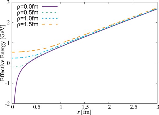
$Effective interaction potential between the heavy quark and the sizable diquark for lower energy states, $|0,0\rangle_{S}$, $|0,1\rangle_{P}$, $|0,2\rangle_{D}$, and $|2,0\rangle_{D}$, which provide the equivalent effective potential. We plot the effective potentials for the diquark sizes $\rho =0$, 0.5, 1.0, and 1.5 fm.$

Fig. 1.

Effective interaction potential between the heavy quark and the sizable diquark for lower energy states, |$|0,0\rangle_{S}$|⁠, |$|0,1\rangle_{P}$|⁠, |$|0,2\rangle_{D}$|⁠, and |$|2,0\rangle_{D}$|⁠, which provide the equivalent effective potential. We plot the effective potentials for the diquark sizes |$\rho =0$|⁠, 0.5, 1.0, and 1.5 fm.

Open in new tab Download slide

3.2. Excitation energy of |${\Lambda_{c}}$| and determination of the diquark size |${\rho}$|

Let us show our result for the excitation spectrum of |$\Lambda_{c}$| as a function of the diquark size. We calculate the energies of the |$1s$|⁠, |$1p$|⁠, |$1d$|⁠, and |$2s$| states by solving the Schrödinger equation given in Eq. (14). The diquark mass is fixed at |$m_{d}=0.5$| GeV/|$c^{2}$|⁠. For the |$1s$| and |$2s$| states, we take the lowest angular momentum configuration |$|\ell_{\rho}, \ell_{\lambda}\rangle_{L} = |0,0\rangle_{S}$| and the |$2s$| state is obtained as the first radial excitation state with |$L=0$|⁠. For the |$1p$| state, we take |$|0,1\rangle_{P}$|⁠, which is the lowest angular momentum configuration for |$L=1$|⁠. The states with higher angular momentum configurations have large rotational energies for the |$\rho$| and |$\lambda$| coordinates. This makes the higher |$\ell_\rho$| and |$\ell_\lambda$| states well separated from the ground state, and the energy difference is large enough to suppress the mixing. We have confirmed with actual numerical calculation that the higher states have essentially no effect on the lowest states and that we can safely neglect the higher angular momentum states. For the |$1d$| state, we take two states, |$| 0,2\rangle_{D}$| and |$|2,0\rangle_{D}$|⁠. We consider the mixing of these two states by calculating the off-diagonal matrix element of the effective potential (11), and obtain the energy eigenstates by diagonalizing the Hamiltonian. We call the lower state |$1d_{1}$| and the higher one |$1d_{2}$|⁠.

In Fig. 2 we show the calculated excitation energies of the |$1p$|⁠, |$2s$|⁠, and |$1d$| states as a function of the diquark size |$\rho$|⁠. These energies are measured from the calculated |$1s$| energy. The excitation energies decrease as the diquark size increases. This is our expected result. For the point-like diquark, which is the case of |$\rho=0$| in the figure, the confinement potential reproducing the meson spectra is so strong that the excitation energies are overestimated compared to the experiments. The size of the diquark reduces the strength of the interaction between the diquark and heavy quark.

$Calculated $\Lambda_{c}$ excitation energies for the $1p$, $2s$, and $1d$ states as a function of the diquark size $\rho$. The energies are measured from the calculated $1s$ state energy. The dotted line stands for the spin-weighted average of the observed excitation energies of $\Lambda_{c}(2595)$ and $\Lambda_{c}(2625)$, 0.330 GeV.$

Fig. 2.

Calculated |$\Lambda_{c}$| excitation energies for the |$1p$|⁠, |$2s$|⁠, and |$1d$| states as a function of the diquark size |$\rho$|⁠. The energies are measured from the calculated |$1s$| state energy. The dotted line stands for the spin-weighted average of the observed excitation energies of |$\Lambda_{c}(2595)$| and |$\Lambda_{c}(2625)$|⁠, 0.330 GeV.

Open in new tab Download slide

With |$\rho \simeq 1.2$| fm, level crossing takes place for the |$|0,2\rangle_{D}$| and |$|2,0\rangle_{D}$| states. The state |$|2,0\rangle_{D}$| has |$\ell_{\rho}=2$|⁠, being a rotational state of the diquark. Thus, the excitation energy is in inverse proportion to the diquark momentum of inertia and decreases as the diquark size increases. Because the states |$|0,2\rangle_{D}$| and |$|2,0\rangle_{D}$| have different angular momenta for the diquark–quark relative motion, the wavefunctions are almost orthogonal. Thus, the mixing between these two states is negligibly small.

We determine the diquark size so as to reproduce the |$1p$| excitation energy |$\Delta E_{1p}$|⁠. In our calculation we do not consider the fine splittings caused by the spin–orbit interaction, since we are interested in the global features of the diquark–quark interaction. Here we compare our results with the experiments by taking the spin-weighted average of the observed masses for the |$LS$| splitting partners, which removes the effect of the spin–orbit interaction in perturbation theory. For the |$1p$| state, |$\Lambda_{c}(2595)$| with |$1/2^{-}$| and |$\Lambda_{c}(2625)$| with |$3/2^{-}$| are the |$LS$| partners. The spin-weighted average of the excitation energy is obtained by |$\Delta E_{\rm ave} = \frac23 \Delta E_{3/2^{-}} + \frac13 \Delta E_{1/2^{-}} = 0.330$| GeV. From Fig. 2, we find that the diquark size |$\rho = 1.1$| fm reproduces the experimental value |$0.330$| GeV. This is consistent with the finding in Refs. [8,15].

3.3. Excited energies of |$\Lambda_{c}$| and |$\Lambda_{b}$| with the determined diquark size

In the previous section, we have determined the diquark size as |$\rho = 1.1$| fm for the diquark mass |$m_{d}=0.5$| GeV/|$c^{2}$| from the excitation energy of the |$1p$| state. Here we discuss the excitation energies of the other states of |$\Lambda_{c}$| and show the excitation energy spectrum of |$\Lambda_{b}$| with the determined diquark size.

In Fig. 3, we present the calculated result of the excitation energies of |$\Lambda_{c}$| and |$\Lambda_{b}$| with the diquark size |$\rho = 1.1$| fm, and there we also show their possible corresponding observed states. As shown in the figure, the |$2s$| states are obtained rather higher than the usual quark model, in which |$\Lambda_{c}(2765)$| is explained as the |$2s$| state. This is because, in our model, the attraction between the diquark and heavy quark gets weaker when two particles are approaching, and thus this reduction of the attractive force is more effective for the |$L=0$| states. Our model fails to reproduce |$\Lambda_{c}(2765)$|⁠. The |$\Lambda_{c}(2765)$| state is a one-star resonance in the Particle Data [25], and its spin and parity are still unknown. Even its isospin is not fixed yet, so that it could be |$\Sigma_{c}$|⁠. Therefore, the isospin of the |$\Lambda_{c}(2765)$| state is the touchstone for the success of our model. If it was |$\Lambda_{c}$|⁠, the diquark picture could not be the case in |$\Lambda_{c}$| excited states. The |$1d$| state is marginally reproduced but is a bit higher than the observed |$\Lambda(2880)$| state.

$Comparison of the calculated $\Lambda_{c}$ and ${\Lambda_{b}}$ excitation energies with the experimental data [25]. The calculation is done with the diquark mass $m_{d}=0.5$ GeV/$c^{2}$ and the diquark size $\rho = 1.1$ fm. The spin and parity of $\Lambda_{c}(2765)$ are not known and its isospin is not fixed yet either.$

Fig. 3.

Comparison of the calculated |$\Lambda_{c}$| and |${\Lambda_{b}}$| excitation energies with the experimental data [25]. The calculation is done with the diquark mass |$m_{d}=0.5$| GeV/|$c^{2}$| and the diquark size |$\rho = 1.1$| fm. The spin and parity of |$\Lambda_{c}(2765)$| are not known and its isospin is not fixed yet either.

Open in new tab Download slide

3.4. The diquark mass dependence

Here we discuss the diquark mass dependence of the diquark size that reproduces the |$1p$| excitation energy of |$\Lambda_{c}$|⁠. In Fig. 4, we show the diquark size appropriate for the |$1p$| excitation of |$\Lambda_{c}$| as a function of the diquark mass. As seen in the figure, if one uses a lighter diquark, the size of the diquark should be larger to reproduce the |$1p$| state of |$\Lambda_{c}$|⁠. Because it is not likely that the diquark size is much larger than 1 fm, a possible diquark mass is larger than 0.5 GeV/|$c^{2}$|⁠.

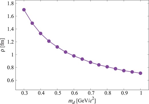
$Diquark mass dependence of the diquark size that reproduces the $1p$ excitation energy of $\Lambda_{c}$.$

Fig. 4.

Diquark mass dependence of the diquark size that reproduces the |$1p$| excitation energy of |$\Lambda_{c}$|⁠.

Open in new tab Download slide

In Fig. 5, we show the calculated |$\Lambda_{c}$| and |$\Lambda_{b}$| excitation energy spectra with the diquark mass |$m_{d}=0.7$| GeV/|$c^{2}$| and diquark size |$\rho=0.88$| fm that reproduce the |$1p$| excitation energy of |$\Lambda_{c}$|⁠. As seen in the figure, the observed excitation energies are reproduced well with this parameter set and this is essentially the same as the calculation with |$m_{d}=0.5$| GeV/|$c^{2}$|⁠, while one sees that with the heavier diquark mass the excitation energies are a bit smaller.

Fig. 5.

Open in new tab Download slide

3.5. |${\Xi_{c}}$| energy spectrum

In this section we discuss the energy spectrum of |$\Xi_{c}$|⁠, which is composed of one charm quark and one strange diquark. The strange diquark is formed by one strange quark and one light (up or down) quark, having spin zero and antisymmetric flavor and color configurations. The values of the potential parameters appearing in Eq. (3) are to be the same as those used in the |$\Lambda_{c}$| calculation.

First of all, we determine the strange diquark mass from the mass difference between the ground states of |$\Lambda_{c}$| and |$\Xi_{c}$|⁠. Here we assume the same size for the strange diquark as the |$ud$| diquark. The |$ud$| diquark mass and diquark size are fixed at 0.5 GeV/|$c^{2}$| and 1.1 fm, respectively. In Fig. 6, we show the |$\Xi_{c}$|–|$\Lambda_{c}$| mass difference for the ground states as a function of the strange diquark mass; the dashed line indicates the observed value of the mass difference, 0.18 GeV/|$c^{2}$|⁠. As shown in the figure, the ground state mass increases as the diquark mass increases. We find that with the strange diquark mass |$m_{ds} = 0.75$| GeV/|$c^{2}$| the observed mass of the lowest-lying |$\Xi_{c}$| state is reproduced. With this strange diquark mass we calculate the |$1p$| excitation energy and obtain 0.30 GeV. This is smaller than the experimental value 0.34 GeV, which is obtained as the spin-weighted average of the excitation energies of |$\Xi_{c}(2790)$| and |$\Xi_{c}(2815)$|⁠.

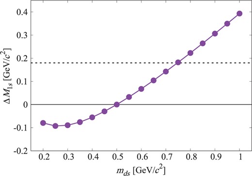
$Mass difference between the ground states of $\Xi_{c}$ and $\Lambda_{c}$ as a function of the strange diquark mass. The size of the strange diquark mass is assumed to be the same as the $ud$ diquark size, which is $\rho =1.1$ fm. The mass of the $ud$ diquark is fixed at 0.5 GeV/$c^{2}$. The horizontal dashed line stands for the observed value of the mass difference of $\Xi_{c}$ and $\Lambda_{c}$.$

Fig. 6.

Mass difference between the ground states of |$\Xi_{c}$| and |$\Lambda_{c}$| as a function of the strange diquark mass. The size of the strange diquark mass is assumed to be the same as the |$ud$| diquark size, which is |$\rho =1.1$| fm. The mass of the |$ud$| diquark is fixed at 0.5 GeV/|$c^{2}$|⁠. The horizontal dashed line stands for the observed value of the mass difference of |$\Xi_{c}$| and |$\Lambda_{c}$|⁠.

Open in new tab Download slide

Next let us determine both the strange diquark mass and size from the masses of the ground and first excited states of |$\Xi_{c}$|⁠. We fix the parameter |$V_{0}$| appearing in Eq. (3) by the lowest-lying |$\Lambda_{c}$| state with the diquark mass 0.5 GeV/|$c^{2}$| and the diquark size 1.1 fm. For the |$1p$| state of |$\Xi_{c}$|⁠, the spin-weighted average mass of |$\Xi_{c}(2790)$| and |$\Xi_{c}(2815)$| gives 2.809 GeV/|$c^{2}$|⁠. In Fig. 7, we show the strange diquark sizes |$\rho_{s}$| that reproduce the masses of the |$1s$| and |$1p$| states of |$\Xi_{c}$| as a function of the strange diquark mass |$m_{ds}$|⁠. From this figure, we find that |$m_{ds} = 0.94$| GeV/|$c^{2}$| and |$\rho_{s}=0.68$| fm reproduce both the masses of the |$1s$| and |$1p$| states. In Fig. 8 we show the calculated |$\Xi_{c}$| excitation energies with this diquark mass and size. Due to a lack of experimental information on the quantum numbers for the higher |$\Xi_{c}$| states, it is not easy to make a further comparison.

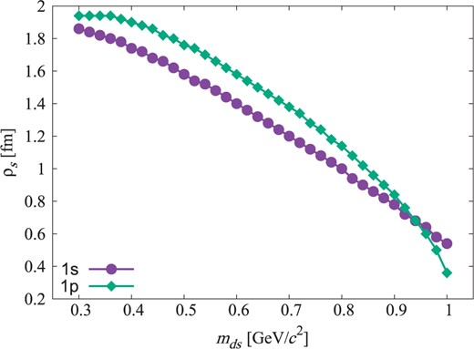
$The diquark mass and size reproducing the masses of the $1s$ and $1p$ states of $\Xi_{c}$. The plot shows that the strange diquark mass $m_{ds}=0.94$ GeV/$c^{2}$ and the strange diquark size $d_{s}=0.68$ fm reproduce both the $1s$ and $1p$ masses of $\Xi_{c}$.$

Fig. 7.

The diquark mass and size reproducing the masses of the |$1s$| and |$1p$| states of |$\Xi_{c}$|⁠. The plot shows that the strange diquark mass |$m_{ds}=0.94$| GeV/|$c^{2}$| and the strange diquark size |$d_{s}=0.68$| fm reproduce both the |$1s$| and |$1p$| masses of |$\Xi_{c}$|⁠.

Open in new tab Download slide

$Comparison of the calculated $\Xi_{c}$ excitation energies with the experimental data [25]. The calculation is done with the strange diquark mass $m_{ds}=0.94$ GeV/$c^{2}$ and strange diquark size $\rho_{s} = 0.68$ fm. We omit $\Xi^{\prime}$ and $\Xi(2645)$ in this figure, because the strange diquark may have spin 1 in these baryons.$

Fig. 8.

Comparison of the calculated |$\Xi_{c}$| excitation energies with the experimental data [25]. The calculation is done with the strange diquark mass |$m_{ds}=0.94$| GeV/|$c^{2}$| and strange diquark size |$\rho_{s} = 0.68$| fm. We omit |$\Xi^{\prime}$| and |$\Xi(2645)$| in this figure, because the strange diquark may have spin 1 in these baryons.

Open in new tab Download slide

4. Conclusion

We have investigated the excitation energy spectra of |$\Lambda_{c}$| and |$\Lambda_{b}$| in a finite-size diquark model, in which the heavy baryon is composed of one heavy quark and one diquark with a finite size. The diquark is treated as a rigid rotor of two light quarks separated at a distance |$\rho$|⁠. The interaction between the heavy quark and the diquark is calculated as the sum of the heavy quark–light quark interactions for the |$\bar {\bf 3}$| color configuration, which is assumed to be half of the quark–antiquark interaction for the color singlet pair. The potential parameter is fixed so as to reproduce the charmonium spectrum with the quark–antiquark interaction.

With the diquark size the interaction between the diquark and heavy quark is reduced at short distances. This makes the excitation energies for the |$L > 0$| states smaller, because the weaker attraction pushes the wavefunction out and the effect of the centrifugal repulsion is suppressed. The present model reproduces the |$1p$| excitation energy of |$\Lambda_{c}$| with the diquark mass 0.5 GeV/|$c^{2}$| and the diquark size 1.1 fm. This diquark size is consistent with the calculation in a Schwinger–Dyson formalism [15]. The quark–diquark model with the diquark size 1.1 fm reproduces well the mass spectra of |$\Lambda_{c}$| and |$\Lambda_{b}$|⁠. This model, however, does not provide |$\Lambda_{c}(2765)$|⁠, which is usually assigned to the |$2s$| state in quark models. Nevertheless, |$\Lambda_{c}(2765)$| is such an uncertain state that its spin–parity is not known, nor is its isospin fixed yet. Thus, detailed information on |$\Lambda_{c}(2765)$| should be necessary for the diquark picture of the heavy baryon. We also discuss the energy spectrum of |$\Xi_{c}$| with the strange diquark. The masses of the |$1s$| and |$1p$| states of |$\Xi_{c}$| can be reproduced with the strange diquark mass |$m_{ds} = 0.94$| GeV/|$c^{2}$| and its size |$\rho_{s}=0.68$| fm.

The calculation done in the present work is quite simple. Nevertheless, the quantitative feature should be reproduced by a simple insight. Thus, the presence of the diquark inside the baryons as an effective constituent should also be reproduced by simple models. If this is not the case, we should be prepared to give up the diquark as an explanation of the excitation mode in the |$\Lambda_{c}$| baryon. In such a case, though, this does not mean that the diquark in the baryon is totally ruled out, nor does it reject the existence of the diquark in the ground state. The diquark could be so fragile that it easily breaks in excitation.

Acknowledgements

The work of D.J. was partly supported by Grants-in-Aid for Scientific Research from JSPS (17K05449).

Appendix A. Construction of states

Each angular momentum state |$|L\rangle$| is a linear combination of the direct products of the angular momentum states for the diquark and the relative motion. We write this product state as |$| \ell_{\rho}m_{\rho}\, \ell_{\lambda}m_{\lambda} \rangle$|⁠, where |$\ell_{\rho}$| and |$m_{\rho}$| (⁠|$\ell_{\lambda}$| and |$m_{\lambda}$|⁠) are the orbital angular momentum and magnetic quantum numbers of the diquark (relative coordinate), respectively. The state with the angular momentum |$L$| for the quark–diquark system combined by the angular momentum states of the diquark and the relative motion with the quantum numbers |$ (\ell_{\rho}, m_{\rho})$| and |$(\ell_{\lambda}, m_{\lambda})$|⁠, respectively, is written with the Clebsch–Gordan coefficient as

\begin{equation} | \ell_{\rho}, \ell_{\lambda} \rangle_{L} = \sum_{m_{\rho}, m_{\lambda}} | \ell_{\rho}m_{\rho}\, \ell_{\lambda}m_{\lambda} \rangle \langle \ell_{\rho}m_{\rho}\, \ell_{\lambda}m_{\lambda} | L M \rangle \end{equation}

(A.1)

The states are written explicitly as

\begin{eqnarray} |0,0 \rangle_{S} &=& |00\,00\rangle \end{eqnarray}

(A.2)

\begin{eqnarray} |2,2 \rangle_{S} &=& \frac{1}{\sqrt 5} \left( | 2 {\, -2}\, 2 {\, +2} \rangle -| 2 {\, -1}\, 2 {\, +1} \rangle + | 20\,20 \rangle - | 2 {\, +1}\, 2 {\, -1} \rangle + | 2 {\, +2}\, 2 {\, -2} \rangle\right) \end{eqnarray}

(A.3)

for the |$S$| states,

\begin{eqnarray} |0,1\rangle_{P} &=& |00\,10 \rangle \end{eqnarray}

(A.4)

\begin{eqnarray} |2,1\rangle_{P} &=& \sqrt{\frac{3}{10}} |2{\,-1}\, 1{\,+1}\rangle - \sqrt{\frac25} |20\,10\rangle + \sqrt{\frac{3}{10}} | 2{\,+1}\, 1{\,-1}\rangle \end{eqnarray}

(A.5)

\begin{eqnarray} |2,2 \rangle_{P} &=& \sqrt\frac25 | 2 {\, -2}\, 2 {\, +2} \rangle - \sqrt\frac1{10} | 2 {\, -1}\, 2 {\, +1} \rangle + \sqrt\frac1{10} | 2 {\, +1}\, 2 {\, -1} \rangle - \sqrt\frac25 | 2 {\, +2}\, 2 {\, -2} \rangle \end{eqnarray}

(A.6)

for the |$P$| states, and

\begin{eqnarray} |0,2\rangle_{D} &=& |00\, 20\rangle \end{eqnarray}

(A.7)

\begin{eqnarray} |2,0\rangle_{D} &=& |20\, 00\rangle \end{eqnarray}

(A.8)

\begin{eqnarray} |2,1\rangle_{D} &=& \frac{1}{\sqrt 2} \left( |2{\, +1}\, 1{\, -1} \rangle - | 2{\, -1}\, 1{\, +1}\rangle \right) \end{eqnarray}

(A.9)

\begin{eqnarray} |2,2 \rangle_{D} &=& \sqrt\frac27 | 2 {\, -2}\, 2 {\, +2} \rangle + \sqrt\frac1{14} | 2 {\, -1}\, 2 {\, +1} \rangle - \sqrt\frac27 | 20\,20 \rangle \nonumber \\ && + \sqrt\frac1{14} | 2 {\, +1}\, 2 {\, -1} \rangle + \sqrt\frac27 | 2 {\, +2}\, 2 {\, -2} \rangle \end{eqnarray}

(A.10)

for the |$D$| states.

Appendix B. Effective potential for quark and diquark interaction

The effective potential appearing in Eqs. (10) and (11) is a linear combination of the matrix element of the interaction potential |$V(\vec r, \rho)$| for the angular momentum state |$| \ell_{\rho}m_{\rho}\, \ell_{\lambda}m_{\lambda} \rangle$|⁠. Here we derive the effective potentials for the Coulomb-type potential |$\displaystyle{v(\vec r_{1} - \vec r_{2}) = \frac{1}{|\vec r_{1} - \vec r_{2}|}}$| and the linear-type potential |$\displaystyle{v(\vec r_{1}- \vec r_{2}) = |\vec r_{1} - \vec r_{2}|}$|⁠.

To obtain the effective potential, we perform the Legendre expansion for the interaction potential |$v(\vec r_{1} - \vec r_{2})$| in terms of the relative angle |$\alpha$| of |$\vec r_{1}$| and |$\vec r_{2}$|⁠:

\begin{equation} v(\vec r_{1}-\vec r_{2}) = \sum_{\ell=0}^{\infty} v_{\ell}(r_{1},r_{2}) P_{\ell}(\cos\alpha). \end{equation}

(B.1)

The Legendre coefficients for the Coulomb- and linear-type potentials are known as

\begin{eqnarray} v_{\ell}(r_{1},r_{2}) = \left\{ \begin{array}{ll} \displaystyle{ \frac{1}{r_{>}} \left( \frac{r_{<}}{r_{>}} \right)^{\ell} } & {\rm for} \ \displaystyle{ v = \frac{1}{|\vec r_{1} - \vec r_{2}|} } \\ \displaystyle{ r_{>} \left[ \frac{1}{2\ell + 3} \left(\frac{r_{<}}{r_{>}}\right)^{\ell+2} - \frac{1}{2\ell-1} \left( \frac{r_{<}}{r_{>}} \right)^{\ell}\right]}& {\rm for} \ \displaystyle{ v =|\vec r_{1} - \vec r_{2}| } \end{array}, \right. \end{eqnarray}

(B.2)

where |$r_{>}$| (⁠|$r_{<}$|⁠) denotes the greater (lesser) of |$|\vec r_{1}|$| and |$|\vec r_{2}|$|⁠.

Using the addition theorem for the Legendre polynomials, we write down the potential with spherical harmonics for the solid angles of |$\vec r_{1}$| and |$\vec r_{2}$|⁠:

\begin{equation} v(\vec r_{1}- \vec r_{2}) = \sum_{\ell=0}^{\infty} v_{\ell}(r_{1},r_{2}) \frac{4\pi}{2\ell +1} \sum_{m=-\ell}^{\ell} Y_{\ell}^{m*}(\Omega_{1}) Y_{\ell}^{m}(\Omega_{2}). \end{equation}

(B.3)

The matrix element of |$v(\vec r_{1}- \vec r_{2})$| of the state |$| \ell_{1}m_{1}\, \ell_{2}m_{2} \rangle$| can be calculated as

\begin{eqnarray} && \langle \ell_{1}^{\prime}m_{1}^{\prime}\, \ell_{2}^{\prime} m_{2}^{\prime} | v(\vec r_{1}- \vec r_{2}) | \ell_{1}m_{1}\, \ell_{2}m_{2}\rangle \nonumber \\ &&\quad{} = \sum_{\ell=0}^{\infty} v_{\ell}(r_{1},r_{2}) \sum_{m=-\ell}^{\ell} \langle \ell_{1}^{\prime} m_{1}^{\prime}|C_{\ell}^{m*}(\Omega_{1}) | \ell_{1} m_{1} \rangle \langle \ell_{2}^{\prime} m_{2}^{\prime} | C_{\ell}^{m}(\Omega_{2}) | \ell_{2} m_{2} \rangle, \end{eqnarray}

(B.4)

where we have defined

\begin{equation} C_{\ell}^{m}(\Omega) = \sqrt \frac{4\pi}{2\ell+1} Y_{\ell}^{m}(\Omega). \end{equation}

(B.5)

The matrix element of |$C_{\ell}^{m}$| is written in terms of the |$3j$| symbol as

\begin{eqnarray} \langle \ell^{\prime} m^{\prime}| C_{L}^{M}| \ell m \rangle \nonumber & =& \sqrt \frac{4\pi}{2L+1} \int d\Omega Y^{m^{\prime}*}_{\ell^{\prime}}(\Omega) Y^{m}_{\ell}(\Omega) Y_{L}^{M}(\Omega) \end{eqnarray}

(B.6)

\begin{eqnarray} &=& (-)^{-m^{\prime}}\sqrt{(2\ell^{\prime} +1)(2\ell+1)} \left(\begin{array}{ccc} \ell^{\prime}& \ell & L \\ 0 & 0 & 0\end{array}\right) \left(\begin{array}{ccc} \ell^{\prime}& \ell & L \\ -m^{\prime} & m & M\end{array}\right)\!. \end{eqnarray}

(B.7)

The |$3j$| symbol is defined by the Clebsch–Gordan coefficient as

\begin{equation} \left(\begin{array}{ccc} j_{1}& j_{2} & J \\ m_{1} & m_{2} & -M\end{array}\right) = \frac{(-)^{j_{1}-j_{2}+M}}{\sqrt{2J+1}} \left\langle j_{1} j_{2} m_{1} m_{2} | JM \right \rangle. \end{equation}

(B.8)

The matrix element has the following properties:

\begin{eqnarray} \langle \ell^{\prime} m^{\prime}| C_{L}^{M*}| \ell m \rangle &=& (-)^{M} \langle \ell^{\prime} m^{\prime}| C_{L}^{-M}| \ell m \rangle \end{eqnarray}

(B.9)

\begin{eqnarray} \langle \ell^{\prime} m^{\prime}| C_{L}^{M}| \ell m \rangle &=& (-)^{m^{\prime} + m} \langle \ell m| C_{L}^{M}| \ell^{\prime} m^{\prime} \rangle . \end{eqnarray}

(B.10)

In the following we list the effective potentials of the Coulomb-type potential for each partial wave:

\begin{eqnarray} _{S}\langle 0,0 | \frac{1}{|\vec r_{1} - \vec r_{2}|} | 0,0 \rangle_{S} &=& \frac{1}{r_{>}} \end{eqnarray}

(B.11)

\begin{eqnarray} _{P}\langle 0,1 | \frac{1}{|\vec r_{1} - \vec r_{2}|} | 0,1 \rangle_{P} &=& \frac{1}{r_{>}} \end{eqnarray}

(B.12)

\begin{eqnarray} _{D}\langle 0,2 | \frac{1}{|\vec r_{1} - \vec r_{2}|} | 0,2 \rangle_{D} &=& \frac{1}{r_{>}} \end{eqnarray}

(B.13)

\begin{eqnarray} _{D}\langle 2,0 | \frac{1}{|\vec r_{1} - \vec r_{2}|} | 2,0 \rangle_{D} &=& \frac{1}{r_{>}} \label{eq:CD2} \end{eqnarray}

(B.14)

\begin{eqnarray} _{D}\langle 2,0 | \frac{1}{|\vec r_{1} - \vec r_{2}|} | 0,2 \rangle_{D} &=& \frac15 \frac{1}{r_{>}} \left(\frac{r_{<}}{r_{>}}\right)^{2} . \end{eqnarray}

(B.15)

We also list the effective potentials of the linear-type potential:

\begin{eqnarray} _{S}\langle 0,0 || \vec r_{1} - \vec r_{2} || 0,0 \rangle_{S} &=& r_{>}\left[1+ \frac{1}{3}\left(\frac{r_{<}}{r_{>}}\right)^{2} \right] \label{eq:LS1} \end{eqnarray}

(B.16)

\begin{eqnarray} _{P}\langle 0,1 || \vec r_{1} - \vec r_{2} || 0,1 \rangle_{P} &=& r_{>} \left[ 1 + \frac{1}{3}\left(\frac{r_{<}}{r_{>}}\right)^{2} \right] \end{eqnarray}

(B.17)

\begin{eqnarray} _{D}\langle 0,2 | {|\vec r_{1} - \vec r_{2}|} | 0,2 \rangle_{D} &=& {r_{>}} \left[1 + \frac{1}{3} \left(\frac{r_{<}}{r_{>}}\right)^{2}\right] \end{eqnarray}

(B.18)

\begin{eqnarray} _{D}\langle 2,0 | {|\vec r_{1} - \vec r_{2}|} | 2,0 \rangle_{D} &=& {r_{>}} \left[1 + \frac{1}{3} \left(\frac{r_{<}}{r_{>}}\right)^{2}\right] \label{eq:LD2} \end{eqnarray}

(B.19)

\begin{eqnarray} _{D}\langle 2,0 | {|\vec r_{1} - \vec r_{2}|} | 0,2 \rangle_{D} &=& - \frac{1}{5} {r_{>}} \left[ \frac13 \left(\frac{r_{<}}{r_{>}}\right)^{2} - \frac17 \left(\frac{r_{<}}{r_{>}}\right)^{4} \right]\!. \end{eqnarray}

(B.20)

In the following, we list the effective potentials of the Coulomb- and linear-type potentials for higher excited states that we do not include in the calculation:

\begin{align} {}_{S}\langle 2,2 | \frac{1}{|\vec r_{1} - \vec r_{2}|} | 2,2 \rangle_{S} =& \frac{1}{r_{>}} \left[ 1 + \frac{2}{7} \left(\frac{r_{<}}{r_{>}}\right)^{2} + \frac{2}{7} \left(\frac{r_{<}}{r_{>}}\right)^{4} \right] \end{align}

(B.21)

\begin{align} _{S}\langle 2,2 | \frac{1}{|\vec r_{1} - \vec r_{2}|} | 0,0 \rangle_{S} =& \frac{1}{\sqrt 5} \frac{1}{r_{>}} \left( \frac{r_{<}}{r_{>}} \right)^{2} \end{align}

(B.22)

\begin{align} _{P}\langle 2,1 | \frac{1}{|\vec r_{1} - \vec r_{2}|} | 2,1 \rangle_{P} &= \frac{1}{r_{>}} \left[1+\frac{1}{5} \left(\frac{r_{<}}{r_{>}}\right)^{2} \right] \end{align}

(B.23)

\begin{align} _{P}\langle 2,1 | \frac{1}{|\vec r_{1} - \vec r_{2}|} | 0,1 \rangle_{P} &= -\frac{\sqrt 2}{5} \frac{1}{r_{>}} \left(\frac{r_{<}}{r_{>}}\right)^{2} \end{align}

(B.24)

\begin{align} _{P}\langle 2,2 | \frac{1}{|\vec r_{1} - \vec r_{2}|} | 2,2 \rangle_{P} &= \frac{1}{r_{>}} \left[ 1 + \frac{1}{7} \left(\frac{r_{<}}{r_{>}}\right)^{2} - \frac{4}{21} \left(\frac{r_{<}}{r_{>}}\right)^{4} \right] \end{align}

(B.25)

\begin{align} _{P}\langle 2,2 | \frac{1}{|\vec r_{1} - \vec r_{2}|} | 0,1 \rangle_{P} &= {}_{P}\langle 2,2 | \frac{1}{|\vec r_{1} - \vec r_{2}|} | 2,1 \rangle_{P} =0 \end{align}

(B.26)

\begin{align} _{D}\langle 2,1 | \frac{1}{|\vec r_{1} - \vec r_{2}|} | 2,1 \rangle_{D} &= \frac{1}{r_{>}} \left[1-\frac{1}{5} \left(\frac{r_{<}}{r_{>}}\right)^{2} \right] \end{align}

(B.27)

\begin{align} _{D}\langle 2,1| \frac{1}{|\vec r_{1} - \vec r_{2}|} | 0,2 \rangle_{D} &= {}_{D}\langle 2,1 | \frac{1}{|\vec r_{1} - \vec r_{2}|} | 2,0 \rangle_{D} = 0 \end{align}

(B.28)

\begin{align} _{D}\langle 2,2 | \frac{1}{|\vec r_{1} - \vec r_{2}|} | 2,2 \rangle_{D} &= \frac{1}{r_{>}} \left[ 1 - \frac{3}{49} \left(\frac{r_{<}}{r_{>}}\right)^{2} + \frac{4}{49} \left(\frac{r_{<}}{r_{>}}\right)^{4} \right] \end{align}

(B.29)

\begin{align} _{D}\langle 2,2 | \frac{1}{|\vec r_{1} - \vec r_{2}|} | 0,2 \rangle_{D} &= - \sqrt\frac2{35} \frac{1}{r_{>}} \left(\frac{r_{<}}{r_{>}}\right)^{2} \end{align}

(B.30)

\begin{align} _{D}\langle 2,2 | \frac{1}{|\vec r_{1} - \vec r_{2}|} | 2,0 \rangle_{D} &= {}- \sqrt\frac2{35} \frac{1}{r_{>}} \left(\frac{r_{<}}{r_{>}}\right)^{2} \end{align}

(B.31)

\begin{align} {}_{D}\langle 2,2| \frac{1}{|\vec r_{1} - \vec r_{2}|} | 2,1 \rangle_{D} &= 0 \end{align}

(B.32)

\begin{align} _{S}\langle 2,2 | {|\vec r_{1} - \vec r_{2}|} | 2,2 \rangle_{S} &= {r_{>}} \left[ 1 + \frac{5}{21} \left(\frac{r_{<}}{r_{>}}\right)^{2} + \frac{2}{77} \left(\frac{r_{<}}{r_{>}}\right)^{6} \right] \end{align}

(B.33)

\begin{align} _{S}\langle 2,2 | {|\vec r_{1} - \vec r_{2}|} | 0,0 \rangle_{S} &= - \frac{1}{\sqrt 5} {r_{>}} \left[ \frac13 \left(\frac{r_{<}}{r_{>}}\right)^{2} - \frac17 \left(\frac{r_{<}}{r_{>}}\right)^{4} \right] \end{align}

(B.34)

\begin{align} {}_{P}\langle 2,1 | {|\vec r_{1} - \vec r_{2}|} | 2,1 \rangle_{P} &= {r_{>}} \left[1+\frac{4 }{15} \left(\frac{r_{<}}{r_{>}}\right)^{2} +\frac{1}{35} \left(\frac{r_{<}}{r_{>}}\right)^{4} \right] \end{align}

(B.35)

\begin{align} _{P}\langle 2,1 | {|\vec r_{1} - \vec r_{2}|} | 0,1 \rangle_{P} &= \frac{\sqrt 2}{5} r_{>} \left[\frac{1}{3} \left(\frac{r_{<}}{r_{>}}\right)^{2} - \frac{1}{7}\left(\frac{r_{<}}{r_{>}}\right)^{4} \right] \end{align}

(B.36)

\begin{align} _{P}\langle 2,2 | {|\vec r_{1} - \vec r_{2}|} | 2,2 \rangle_{P} &= {r_{>}} \left[ 1 + \frac{2}{7} \left(\frac{r_{<}}{r_{>}}\right)^{2} + \frac{1}{21}\left(\frac{r_{<}}{r_{>}}\right)^{4} -\frac{4}{3\cdot 7 \cdot11} \left(\frac{r_{<}}{r_{>}}\right)^{6} \right] \end{align}

(B.37)

\begin{align} {}_{P}\langle 2,2 | {|\vec r_{1} - \vec r_{2}|} | 0,2 \rangle_{P} &= {}_{P}\langle 2,2 | {|\vec r_{1} - \vec r_{2}|} | 2,0 \rangle_{P} = 0 \end{align}

(B.38)

\begin{align} {}_{D}\langle 2,1 | {|\vec r_{1} - \vec r_{2}|} | 2,1 \rangle_{D} &= {r_{>}} \left[1+\frac{2}{5} \left(\frac{r_{<}}{r_{>}}\right)^{2} - \frac{1}{35} \left(\frac{r_{<}}{r_{>}}\right)^{4} \right] \end{align}

(B.39)

\begin{align} {}_{D}\langle 2,1 | {|\vec r_{1} - \vec r_{2}|} | 0,2 \rangle_{D} &= {}_{D}\langle 2,1 | {|\vec r_{1} - \vec r_{2}|} | 2,0 \rangle_{D} = 0 \end{align}

(B.40)

\begin{align} {}_{D}\langle 2,2 | {|\vec r_{1} - \vec r_{2}|} | 2,2 \rangle_{D} &= {r_{>}} \left[ 1 + \frac{4\cdot 13}{3\cdot 7^{2}} \left(\frac{r_{<}}{r_{>}}\right)^{2} -\frac{1}{7^{2}} \left(\frac{r_{<}}{r_{>}}\right)^{4} +\frac{4}{7^{2} \cdot 11} \left(\frac{r_{<}}{r_{>}}\right)^{6} \right] \end{align}

(B.41)

\begin{align} {}_{D}\langle 2,2 | {|\vec r_{1} - \vec r_{2}|} | 0,2 \rangle_{D} &= \sqrt\frac2{35} {r_{>}} \left[\frac13\left(\frac{r_{<}}{r_{>}}\right)^{2} - \frac17\left(\frac{r_{<}}{r_{>}}\right)^{4} \right] \end{align}

(B.42)

\begin{align} _{D}\langle 2,2 | {|\vec r_{1} - \vec r_{2}|} | 2,0 \rangle_{D} &= \sqrt\frac2{35} {r_{>}} \left[\frac13\left(\frac{r_{<}}{r_{>}}\right)^{2} - \frac17\left(\frac{r_{<}}{r_{>}}\right)^{4} \right] \end{align}

(B.43)

\begin{align} &\quad _{D}\langle 2,2 | {|\vec r_{1} - \vec r_{2}|} | 2,1 \rangle_{D} = 0. \end{align}

(B.44)

References

[1]

Ida

and

Kobayashi

Prog. Theor. Phys.

846

(

1966

). (

http://dx.doi.org/10.1143/PTP.36.846

)

Crossref

Search ADS

[2]

Lichtenberg

D. B.

and

Tassie

L. J.

Phys. Rev.

155

1601

(

1967

). (

http://dx.doi.org/10.1103/PhysRev.155.1601

)

Crossref

Search ADS

[3]

Anselmino

Predazzi

Ekelin

Fredriksson

and

Lichtenberg

D. B.

Rev. Mod. Phys.

1199

(

1993

). (

http://dx.doi.org/10.1103/RevModPhys.65.1199

)

Crossref

Search ADS

[4]

Jaffe

R. L.

Phys. Rept.

409

(

2005

) [

Nucl. Phys. Proc. Suppl.

http://dx.doi.org/10.1016/j.nuclphysbps.2005.01.058

142

343

(

2005

)] (

https://doi.org/10.1016/j.physrep.2004.11.005

)

Crossref

Search ADS

[5]

Hess

Karsch

Laermann

and

Wetzorke

Phys. Rev. D

111502

(

1998

). (

http://dx.doi.org/10.1103/PhysRevD.58.111502

)

Crossref

Search ADS

[6]

Babich

et al. ,

J. High Energy Phys.

086

(

2006

). (

http://dx.doi.org/10.1088/1126-6708/2006/01/086

)

Crossref

Search ADS

[7]

Orginos

Proc. Sci.

LAT2005

054

(

2005

[8]

Alexandrou

de Forcrand

and

Lucini

Phys. Rev. Lett.

222002

(

2006

). (

http://dx.doi.org/10.1103/PhysRevLett.97.222002

)

Crossref

Search ADS

PubMed

[9]

Goldstein

G. R.

and

Maharana

Nuovo Cimento A

393

(

1980

). (

http://dx.doi.org/10.1007/BF02904682

)

Crossref

Search ADS

[10]

Lichtenberg

D. B.

Phys. Rev.

178

2197

(

1969

). (

http://dx.doi.org/10.1103/PhysRev.178.2197

)

Crossref

Search ADS

[11]

Lichtenberg

D. B.

Namgung

Predazzi

and

Wills

J. G.

Phys. Rev. Lett.

1653

(

1982

). (

http://dx.doi.org/10.1103/PhysRevLett.48.1653

)

Crossref

Search ADS

[12]

Liu

K. F.

and

Wong

C. W.

Phys. Rev. D

170

(

1983

). (

http://dx.doi.org/10.1103/PhysRevD.28.170

)

Crossref

Search ADS

[13]

Ebert

Faustov

R. N.

and

Galkin

V. O.

Phys. Rev. D

034026

(

2005

). (

http://dx.doi.org/10.1103/PhysRevD.72.034026

)

Crossref

Search ADS

[14]

Ebert

Faustov

R. N.

and

Galkin

V. O.

Phys. Lett. B

659

612

(

2008

). (

http://dx.doi.org/10.1016/j.physletb.2007.11.037

)

Crossref

Search ADS

[15]

Imai

and

Suganuma

J. Mod. Phys.

790

(

2016

). (

http://dx.doi.org/10.4236/jmp.2016.78073

)

Crossref

Search ADS

[16]

Hernández

Nieves

and

Verde-Velasco

J. M.

Phys. Lett. B

666

150

(

2008

). (

https://doi.org/10.1016/j.physletb.2008.07.007

)

Crossref

Search ADS

[17]

Wang

and

Zhu

R. L.

[arXiv:1704.00179]. [hep-ph] [Search inSPIRE].

[18]

Kim

Jido

and

Lee

S. H.

Phys. Rev. C

025204

(

2011

). (

http://dx.doi.org/10.1103/PhysRevC.84.025204

)

Crossref

Search ADS

[19]

Jaffe

R. L.

Phys. Rev. D

267

(

1977

). (

http://dx.doi.org/10.1103/PhysRevD.15.267

)

Crossref

Search ADS

[20]

Jaffe

R. L.

Phys. Rev. D

281

(

1977

). (

http://dx.doi.org/10.1103/PhysRevD.15.281

)

Crossref

Search ADS

[21]

Jido

and

Sakashita

Prog. Theor. Exp. Phys.

2016

083D02

(

2016

). (

http://dx.doi.org/10.1093/ptep/ptw113

)

Crossref

Search ADS

[22]

Eichten

Gottfried

Kinoshita

Kogut

J. B.

Lane

K. D.

and

Yan

T. M.

Phys. Rev. Lett.

369

(

1975

);

1276

(

1976

) [erratum]. (

http://dx.doi.org/10.1103/PhysRevLett.34.369

) (

http://dx.doi.org/10.1103/PhysRevLett.36.1276

)

Crossref

Search ADS

[23]

Mukherjee

S. N.

Nag

Sanyal

Morii

Morishita

and

Tsuge

Phys. Rept.

231

201

(

1993

). (

http://dx.doi.org/10.1016/0370-1573(93)90010-B

)

Crossref

Search ADS

[24]

Quigg

and

Rosner

J. L.

Phys. Rept.

167

(

1979

). (

http://dx.doi.org/10.1016/0370-1573(79)90095-4

)

Crossref

Search ADS

[25]

Patrignani

et al. [

Particle Data Group

Chin. Phys. C,

100001

(

2016

)

and 2017 update

. (

http://dx.doi.org/10.1088/1674-1137/40/10/100001

)

Crossref

Search ADS

This is an Open Access article distributed under the terms of the Creative Commons Attribution License (http://creativecommons.org/licenses/by/4.0/), which permits unrestricted reuse, distribution, and reproduction in any medium, provided the original work is properly cited.

Download all slides

Month:	Total Views:
December 2017	258
January 2018	44
February 2018	19
March 2018	47
April 2018	21
May 2018	15
June 2018	12
July 2018	11
August 2018	10
September 2018	12
October 2018	6
November 2018	12
December 2018	15
January 2019	22
February 2019	19
March 2019	20
April 2019	23
May 2019	5
June 2019	12
July 2019	16
August 2019	21
September 2019	43
October 2019	9
November 2019	14
December 2019	11
January 2020	11
February 2020	9
March 2020	9
April 2020	1
May 2020	3
June 2020	15
July 2020	8
August 2020	6
September 2020	13
October 2020	9
November 2020	9
December 2020	4
January 2021	4
February 2021	17
March 2021	6
April 2021	10
May 2021	7
June 2021	13
July 2021	13
August 2021	9
September 2021	4
October 2021	3
November 2021	10
December 2021	4
January 2022	2
February 2022	3
March 2022	12
April 2022	8
May 2022	5
June 2022	4
July 2022	7
August 2022	10
September 2022	1
October 2022	2
November 2022	1
December 2022	8
January 2023	14
February 2023	4
March 2023	7
April 2023	11
May 2023	2
July 2023	14
August 2023	18
September 2023	5
October 2023	4
November 2023	5
December 2023	3
January 2024	7
February 2024	6
March 2024	5
April 2024	3
May 2024	7
June 2024	12
July 2024	4
August 2024	1
September 2024	3
October 2024	8
November 2024	6
December 2024	6
January 2025	7
February 2025	4
March 2025	17
April 2025	7
May 2025	2

Article Contents

Excitation energy spectra of the |$\Lambda_{c}$| and |$\Lambda_{b}$| baryons in a finite-size diquark model

Abstract

1. Introduction

2. Formulation

3. Results

3.1. Effective potential between diquark and heavy quark

3.2. Excitation energy of |${\Lambda_{c}}$| and determination of the diquark size |${\rho}$|

3.3. Excited energies of |$\Lambda_{c}$| and |$\Lambda_{b}$| with the determined diquark size

3.4. The diquark mass dependence

3.5. |${\Xi_{c}}$| energy spectrum

4. Conclusion

Acknowledgements

Appendix A. Construction of states

Appendix B. Effective potential for quark and diquark interaction

References

Citations

Views

Altmetric

Email alerts

Astrophysics Data System

Citing articles via

Latest

Most Read

Most Cited

Article Contents

Excitation energy spectra of the |$\Lambda_{c}$| and |$\Lambda_{b}$| baryons in a finite-size diquark model Open Access

Abstract

1. Introduction

2. Formulation

3. Results

3.1. Effective potential between diquark and heavy quark

3.2. Excitation energy of |${\Lambda_{c}}$| and determination of the diquark size |${\rho}$|

3.3. Excited energies of |$\Lambda_{c}$| and |$\Lambda_{b}$| with the determined diquark size

3.4. The diquark mass dependence

3.5. |${\Xi_{c}}$| energy spectrum

4. Conclusion

Acknowledgements

Appendix A. Construction of states

Appendix B. Effective potential for quark and diquark interaction

References

Citations

Views

Altmetric

Email alerts

Astrophysics Data System

Citing articles via

Latest

Most Read

Most Cited

This Feature Is Available To Subscribers Only

Excitation energy spectra of the |$\Lambda_{c}$| and |$\Lambda_{b}$| baryons in a finite-size diquark model