Jet-induced jammed states of granular jet impacts Open Access

Abstract

1. Introduction

Non-equilibrium phenomena induced by impacts have been extensively studied in various contexts, such as nuclear reactions [1–3], nanotechnology [4,5], water-bells [6,7], and granular flows [8–18]. Crater morphology is studied via an impact process of a free-falling water drop or a grain onto a granular layer [9,10], while a sinking grain produces a sand jet [11]. The impact of a granular jet on a target produces a sheet-like scattered pattern or a cone-like pattern, depending on the ratio of the target diameter and the jet diameter [8], which is also found in water-bell experiments with low surface tensions [6,7].

Cheng et al. suggested that the fluid state of a granular jet after an impact is similar to the Quark Gluon Plasma(QGP), which behaves as a perfect fluid through their experiment [8]. Recently, we reported that the shear viscosity during the impact is well described by the kinetic theory of the granular gas [19–24], though the small shear stress observed in the experiment is reproduced through our three-dimensional (3D) simulation [12,13]. Because the shear viscosity, at least, for 3D is not anomalous, the correspondence between a granular flow and QGP would be superficial.

To discuss the fluid state of granular jets, we need to know the details of rheology of moderate dense granular flows. A typical situation of the study for a dense granular flow is the flow on an inclined plane [25–27]. Bagnold proposed the constitutive equation for dense granular flows that the shear stress is proportional to the square of the shear rate [25], so-called Bagnold's scaling, which has been verified experimentally [26] and numerically [27,28] under several conditions such as the flow down an inclined plane. Dense granular flows, however, have more variety of rheological constitutive equations for flows on inclined planes [29–33]. A conventional one would be the constitutive equation presented by Jop and coworkers [30], where the effective friction constant, defined as the ratio of shear stress to pressure, saturates from a static value at zero shear rate to a maximum value as the shear rate increases. The power-law friction law, which is also different from Bagnold's scaling for dense granular flows, is proposed via extensive simulations [34–37].

A granular system has rigidity above a critical value of density |$\phi _{\mathrm {J}}$| and does not have any rigidity below |$\phi _{\mathrm {J}}$|⁠. This sudden change of the rigidity is known as the jamming transition [38–51]. The jamming is not only investigated in systems of grains, but also of colloidal suspensions [52] or foams [53]. Here, |$\phi _{\mathrm {J}}$| decreases as the friction constant |$\mu _{\mathrm {p}}$| of grains increases. Moreover, it seems that there are two fictitious jamming points in addition to the true jamming point for finite |$\mu _{\mathrm {p}}$| [39]. Critical exponents of the divergence of the pressure and the shear viscosity near the transition are extensively discussed [39–51].

The aim of this paper is to investigate the rheological properties for two-dimensional (2D) granular jet impacts. Although some previous numerical studies on granular jets used 2D simulations to reproduce 3D experiments for computational efficiency [14–16], it is unclear whether the rheological properties in 2D granular jets are qualitatively the same as those in 3D. Therefore, it is necessary to clarify the qualitative difference between 2D and 3D granular jets. Because grains are easily packed through the impact in 2D, the system would be near the jammed state. Thus, we can investigate rheological properties of very dense granular fluids after the impact of granular jet flow, which cannot be achieved by 3D simulations and experiments. As a result, correlated flows appear in 2D granular jets, while uncorrelated flows characterized by the granular kinetic theory are realized in 3D jets. This is another advantage for the visualization to use the 2D system even for experiments to learn the detailed properties of particles in granular jets, such as contact networks (force chains) and the effect of crystallization for the mono-disperse case. We also stress that it is easy to perform 2D or one-layer experiments for granular jets.

In this paper, we perform 2D simulations for the granular jet in terms of the discrete element method (DEM) [54]. This paper is complementary to the previous 2D DEM study [16], and hard core simulations supplemented by the simulation of a perfect fluid model [15]. Indeed, although Huang et al. reported the relevant role of the contact stress in a 2D granular jet, they were not interested in the critical behavior of jammed grains induced by the jet. Guttenberg suggested that the friction constant does not play a significant role, at least in the scattering angle [14], while the effects on the jammed state induced by jets were not studied in his paper.

This paper is organized as follows: After the introduction of our numerical model in Sect. 2, we analyze the profile of the local stress tensor, the area fraction, and the granular temperature. We also discuss the rheology of the granular jets for the frictionless case in 2D to compare their behavior with the jamming transition for a bi-disperse frictionless case. The effect of the friction constant is discussed in Sect. 4. In Sect. 5, our numerical results for a mono-disperse case are shown, and the paper is concluded in Sect. 6. In Appendix A, we comment on the artificial burst-like flow in 2D, which appears in the case of large |$\mu _{\mathrm {p}}$| for soft grains. In Appendix B, we discuss the effect of the inhomogeneity of the temperature to Bagnold's scaling in terms of the method of Green's function.

2. Model

We adopt DEM to simulate the jet [54]. We mainly focus on bi-dispersed soft core particles of diameter |$d$| and |$0.8d$| with the same mass |$m$| to avoid crystallization. When the particle |$i$| at position |$\textbf {r}_i$| and the particle |$j$| at |$\textbf {r}_j$| are in contact, the normal force |$F^{\mathrm {n}}_{ij}$| is given by |$F^{\mathrm {n}} _{ij} \equiv F_{ij} ^{\rm (el)} + F_{ij} ^{\rm (vis)}$|⁠, with |$F_{ij}^{\mathrm {(el)}} \equiv k_{\rm n}(R_i + R_j - r_{ ij})$| and |$F_{ ij} ^{\mathrm {(vis)}} \equiv -\eta _{\rm n}(\textbf {g}_{ ij} \cdot \hat {\textbf {r}}_{ ij})$|⁠, where |$r_{ij} \equiv |\textbf {r}_{i} - \textbf {r}_{j}|$| and |$\textbf {g}_{ij} \equiv \textbf {v}_{ i} - \textbf {v}_{ j}$|⁠, with the velocity |$\textbf {v}_i$| and the radius |$R_i$| of the particle |$i$|⁠. The tangential force is given by |$F^{\mathrm {t}} _{ij} \equiv \min \{ |\tilde {F^{\rm t} _{ij}}|, \mu _{\rm p} F_{ij}^{\rm n} \}{\rm sgn}(\tilde {F}_{ij}^{\rm t}) $|⁠, where the sign function is defined to be |${\rm sgn}(x)=1$| for |$x\ge 0$| and |${\mathrm {sgn}}(x)=-1$| otherwise, |$\tilde {F^{\mathrm {t}} _{ij}} \equiv k_{\rm t} \delta ^t _{ij} - \eta _{\rm t} \dot {\delta }_{ij} ^{\rm t}$| with the tangential overlap |$\delta ^{\mathrm {t}} _{ij}$| and the tangential component of relative velocity |$\dot {\delta }^{\mathrm {t}} _{ij}$| between the |$i$|th and |$j$|th particles. We examine the value of |$\mu _{\mathrm {p}}$| from |$\mu _{\mathrm {p}} = 0.2$| to |$1.0$|⁠. Here, we adopt parameters |$k_{\mathrm {n}} = 4.98 \times 10^2 mu_0 ^2 /d^2$|⁠, |$\eta _{\mathrm {n}} = 2.88 u_0 /d$|⁠, with the incident velocity |$u_0$| for the frictionless case and |$\mu _{\mathrm {p}} = 0.2$|⁠. The value |$\mu _{\mathrm {p}} = 0.2$| is close to the experimental value for nylon spheres [55]. We use |$k_{\mathrm {n}} = 1.99 \times 10^3 mu_0 ^2 /d^2, \eta _{\mathrm { n}} = 5.75 u_0 /d$| for |$\mu _{\mathrm {p}} = 0.4$|⁠, and |$k_{\mathrm {n}} = 7.96\times 10^2 mu_0 ^2 /d^2, \eta _{\mathrm { n}} = 10.15 u_0 /d$| for |$\mu _{\mathrm {p}} = 1.0$|⁠. These sets of parameters imply that the duration times are, respectively, |$t_{\mathrm {c}} = 0.10 d/u_0$| for the frictionless case and |$\mu _{\mathrm {p}} = 0.2$|⁠, |$t_c = 0.05 d/u_0$| for |$\mu _{\mathrm {p}} = 0.4$|⁠, and |$t_c = 0.01d/u_0$| for |$\mu _{\mathrm {p}} = 1.0$|⁠; the restitution coefficient for a normal impact is unchanged at |${e} = 0.75$| for the frictionless case and for all |$\mu _{\mathrm {p}}$|⁠. The reason we adopt these parameters for large |$\mu _{\mathrm {p}}$| is that many overlaps among grains lead to the artificial burst-like flow if we adopt the identical |$t_{\mathrm {c}}$| to frictionless case, as is shown in Appendix A. For the tangential parameters, we choose |$k_{\mathrm {t}} = 0.2 k_{\mathrm { n}}, \eta _{\rm t} = 0.5 \eta _{\mathrm { n}}$|⁠. We adopt the second-order Adams–Bashforth method for the time integration of Newton's equation, with the time interval |$\Delta t = 0.02 t_{\mathrm {c}}$|⁠.

An initial configuration is generated as follows: We prepare a triangular lattice with distance between grains |$1.1d$| and remove particles randomly to reach the desired density. We control the initial area fraction |$\phi _0 / \phi _{\mathrm {ini}} \equiv \tilde {\phi _0}$| before the impact as |$0.30 \leq \tilde {\phi _0} \leq 0.90$|⁠, with the initial area fraction before the removal |$\phi _{\mathrm {ini}} = 0.612, 0.780$| for the bi-disperse and the mono-disperse case, respectively, and 8,000 particles are used. We average numerical data over the time |$180.0 \leq tu_0/d < 300.0$| after the impact. The initial granular temperature, which represents the fluctuation of the particles’ motion, is zero. The wall consists of particles in one layer with the same diameter |$d$| and the same mass |$m$|⁠, which are connected to each other and with their own initial positions via a spring and dashpot with the spring constant |$k_{\mathrm {w}} = 10.0 mu_0 ^2 /d^2$| and the dashpot constant |$\eta _{\mathrm {w}} = 5.0 \eta _{\mathrm { n}}$|⁠, respectively.

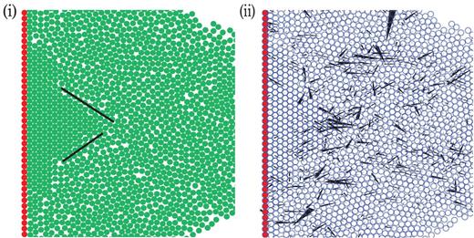
A typical snapshot of our simulation and that of the contact force network are shown in Fig. 1 (i) and (ii), respectively. Blue, green, and red particles denote grains with diameter |$0.8d$| and |$d$|⁠, and wall particles, respectively, in Fig. 1(i), and the corresponding contact force network among grains is visualized as black-colored arrows in Fig. 1(ii). It is easily found that the contact force network emerges during the impact. It should be noted that the average coordination number |$Z \equiv \sum _{i \ne j} \Theta (R_i + R_j - r_{ij})/N \simeq 0.526$|⁠, and 71.5% of particles are not in contact in the region |$0<x\leq 10$| and |$|y| < R_{\mathrm {tar}}$|⁠, where |$\Theta (x)$| and |$N$| represent the Heaviside function and the number of particles in the region.

Fig. 1.

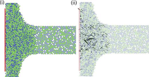
(i) A typical snapshot of the simulation for the frictionless case with |$\tilde {\phi }_0 = 0.90$|⁠. Blue particles and green particles denote grains with diameter |$0.8d$| and |$d$|⁠, respectively, and red particles are wall particles. (ii) The corresponding contact forces among grains are visualized as black-colored arrows. The average coordination number |$Z \simeq 0.526$| and 71.5% of particles are not in contact in the region |$0<x\leq 10$| and |$|y| < R_{\mathrm {tar}}$|⁠.

Open in new tabDownload slide

We evaluate physical quantities near the wall in two regions: |$0<x\leq 5d$| and |$5d < x \leq 10d$|⁠, which we call the (a) and (b) layers in the following, respectively. We use |$R_{\mathrm {jet}} /d = 15.0$| and |$R_{\mathrm {tar}} /R_{\mathrm { jet}} = 2.2$| with the jet radius |$R_{\mathrm {jet}}$|⁠. We adopt Cartesian coordinates, where |$y=0$| is chosen to be the jet axis, and divide the calculation region in the |$y$| direction into |$y = -5\Delta y, - 4 \Delta y, \ldots , 0, \ldots , 5\Delta y$|⁠, with |$\Delta y \equiv R_{\mathrm {tar}} /5$|⁠. Then we estimate physical quantities in the corresponding mesh region with |$k\Delta y < y < (k+1)\Delta y$| (⁠|$k = -5, -4, \ldots ,4$|⁠). Numerical data are averaged over ten initial configurations with the same |$\tilde {\phi }_0$| and error bars in figures denote their variance.

3. Rheology of granular jets for the frictionless case

In this section, our numerical results for granular jets for 2D frictionless cases are presented. The results for frictional grains will be reported in Sect. 4. In Sect. 3.1, the existence of the dead zone and the profile of the area fraction are discussed. After showing profiles of the stress tensor in the (a) or (b) layer in Sect. 3.2, we evaluate the equation of state and constitutive equation to compare our system with the critical behavior of the jamming in Sects. 3.3 and 3.4, respectively.

3.1 Existence of the dead zone and the profile of the area fraction

The Chicago group suggested the existence of the dead zone near the target, where the motion of the grains is frozen [14, 15]. Ellowitz et al. suggested that the dead zone exists in the sense that the velocities of grains are close to zero in Ref. [15]. However, as is shown in our previous paper [13], although the velocity of grains at the center is small, the fluctuation of the velocity, i.e. the granular temperature |$T_{\mathrm {g}}$|⁠, defined by |$T_{\mathrm {g}} \equiv \sum _{i \in {\rm c}} m\textbf {u}_i ^2 / DN_{\rm c} $| with the number of grains |$N_{\mathrm {c}}$| in the mesh |$c$| and the spatial dimensions |$D$|⁠, is largest at the center in 3D |$(D = 3)$|⁠.

On the other hand, we verify the existence of the actual frozen layer (a), i.e. |$T_{\mathrm {g}} \simeq 0$|⁠. The fluctuation of the grain velocity in the (a) layer is suppressed, while the motion is not frozen in the (b) layer for 2D granular jets |$(D = 2)$|⁠. The numerical data for |$T_{\mathrm {g}}$| in 2D for the frictionless case are shown in Fig. 2(i). |$T_{\mathrm {g}}$| is smallest at the center |$y \simeq 0$| in the (a) layer, which cannot be found in our previous 3D study (see Fig. 2 in Ref. [13]), while |$T_{\mathrm {g}}$| is largest at |$y \simeq 0$| in the (b) layer. In a very recent paper by Chicago group, it is suggested that the dead zone also exists in 3D experiments by introducing the effective temperature, whose definition is not explicitly written [17].¹

Fig. 2.

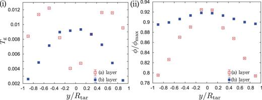
The profiles of |$T_{\mathrm {g}}$| and |$\phi /\phi _{\max }$| for the frictionless case with |$\tilde {\phi }_0 = 0.90$| are shown in (i) and (ii), respectively. There exists the dead zone in the (a) layer, which is denoted by red empty squares. Blue filled squares denote |$T_{\mathrm {g}}$| in the (b) layer, where the dead zone does not exist. Grains are well packed in 2D: |$0.79 < \phi /\phi _{\max } < 0.94$|⁠. Note that |$\phi $| in the (b) layer remains nearly constant compared with the (a) layer, because grains in the (b) layer are not compressed, while those inthe (a) layer are ejected after the compression.

Open in new tabDownload slide

The profile of the packing fractions divided by |$\phi _{\max }$| with |$\phi _{\max } \equiv \pi /(2\sqrt {3})\simeq 0.907$| in 2D is shown in Fig. 2(ii) for the frictionless case. In 3D, the packing fraction divided by |$\phi _{\max }^{3D} \simeq 0.740$| ranges within |$0.30 < \phi /\phi _{\max }^{3D} < 0.75$|⁠. Compared with 3D, grains in 2D are well packed: |$0.79 < \phi /\phi _{\max } < 0.94$|⁠. Note that |$\phi $| in the (b) layer is almost independent of the position, while |$\phi $| in the (a) layer strongly depends on the position.

3.2 Profile of the stress tensor

The profiles of the stress tensor for the (a) and (b) layers of frictionless grains are shown in Fig. 3 (i) and (ii), respectively. We stress that there exists a large normal stress difference between |$\sigma _{xx}$| and |$\sigma _{yy}$| in each layer as in the 3D case [12].

Fig. 3.

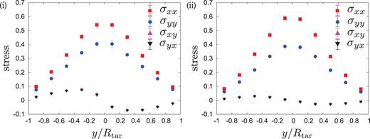
The profiles of the stress tensor in the (a) and (b) layers for |$\tilde {\phi }_0 = 0.90$| are shown in (i) and (ii), respectively. There exist large normal stress differences between |$\sigma _{xx}$| and |$\sigma _{yy}$|⁠, and the shear stress is much smaller than the normal stress in the (b) layer, though it is not so small in the (a) layer.

Open in new tabDownload slide

Ellowitz et al. suggested that the profile of the velocity and the pressure for the granular jet are reproducible from the simulation of a perfect fluid [15], but our result may not support their claim. Indeed, the shear stress looks small but finite. Moreover, the large normal stress difference exists in both layers, which does not exist in the perfect fluid. We should note that they have not discussed the stress tensor itself in detail, though they reproduce some similar features through their hard core simulation. In addition, Huang et al. indicated the relevant role of the contact stress in their DEM simulation, which may be an indirect objection to the perfect fluidity of the jet flow [16].

3.3 Equation of state

Let us discuss the equation of state for the 2D granular jet impact. We estimate the strain rate |$D_{xy} \equiv (\partial \bar {v}_y / \partial x + \partial \bar {v}_x / \partial y) /2$| as |$\partial \bar {v}_y (\Delta x /2, y) / \partial x \simeq (\bar {v}_y(3\Delta x /4, y) - \bar {v}_y(\Delta x /4, y)) / (\Delta x /2)$|⁠, |$\partial \bar {v}_y (3\Delta x / 2, y) / \partial x \simeq (\bar {v}_y(7\Delta x /4, y) - \bar {v}_y(5\Delta x /4, y)) / (\Delta x /2)$| and |$\partial \bar {v}_x (x,y) / \partial y \simeq (\bar {v}_x(x, y + \Delta y/2) - \bar {v}_x (x, y - \Delta y/2)) / \Delta y$|⁠. Since physical quantities are evaluated near the wall, the mesh |$0 < x < \Delta x$| is divided into |$0 < x \leq \Delta x /2$| and |$\Delta x / 2 < x < \Delta x$|⁠, and |$\Delta x \leq x < 2\Delta x$| is divided into |$\Delta x \leq x < 3\Delta x /2$| and |$3 \Delta x /2 \leq x < 2\Delta x$| to calculate |$\partial \bar {v}_y (\Delta x/2, y) / \partial x$| and |$\partial \bar {v}_y (3\Delta x /2, y) / \partial x$|⁠. |$-R_{\mathrm {tar}}<y<R_{\rm tar}$| is divided into |$-11 \Delta y /2 < y < -9 \Delta y/2, -9 \Delta y /2 < y < -7 \Delta y/2, \ldots , 9 \Delta y /2 < y < 11 \Delta y/2$| to calculate |$\partial \bar {v}_x (x, y) / \partial y$|⁠.

We follow the analysis in Ref. [34]. Here, we introduce two dimensionless numbers consisting of pressure: |$I_{\mathrm {T}} \equiv \sqrt {T_{\rm g} / Pd^2}$| and |$I_{\mathrm {s}} \equiv D_{xy} \sqrt {m/P}$|⁠, with pressure |$P \equiv (\sigma _{xx} + \sigma _{yy}) /2$|⁠. We plot numerical data on the |$\phi $| vs |$I_{\mathrm {T}}$| plane and the |$\phi $| vs |$I_{\rm s}$| plane in Fig. 4 (i) and (ii), respectively. Comparing |$\phi $| in the (a) with (b) layers against the identical |$I_{\mathrm {T}}$|⁠, |$\phi $| in the (b) layer has a little larger value than |$\phi $| in the (a) layer at the same |$I_{\mathrm {T}}$|⁠, while all |$\phi $| against |$I_{\mathrm {s}}$| are collapsed on a universal curve (Fig. 4(ii)).

Fig. 4.

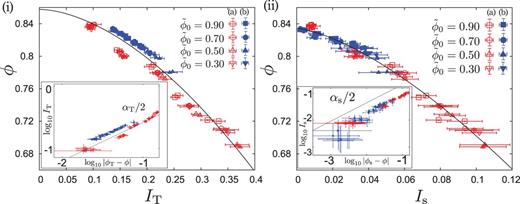
Numerical data for the bi-disperse case of frictionless grains are plotted on the |$\phi $| vs |$I_{\mathrm {T}}$| plane (i) and |$\phi $| vs |$I_{\mathrm {s}}$| plane (ii) of the main figure. Red and blue points denote data of the (a) and (b) layers for several |$\tilde {\phi }_0$|⁠, respectively. The corresponding solid lines in the figures are fitting equations (2) and (3). The insets denote numerical data for (i) |$\log _{10} I_{\mathrm {T}}\ {\rm vs}\ \log _{10} |\phi _{\rm T} - \phi |$| and (ii) |$\log _{10} I_{\rm s}\ {\mathrm {vs}}\ \log _{10} |\phi _{\rm s} - \phi |$| to examine how good the fitting results are.

Open in new tabDownload slide

On the other hand, Hatano demonstrated an elegant scaling law in the vicinity of |$\phi _{\mathrm {J}}$|⁠, where the corresponding exponents are estimated as |$\alpha _{\mathrm {s}} = 2.8$| and |$\alpha _{\mathrm {T}} = 1.7$| from his data of the jamming transition [48]. Otsuki and Hayakawa showed the phenomenological explanation of the critical behavior near |$\phi _{\mathrm {J}}$| and they predicted |$\alpha _{\mathrm {s}} = 4.0$| and |$\alpha _{\mathrm {T}} = 2.0$| [44,47]. It should be stressed that the critical scaling of the jamming transition is analyzed in the |$D_{xy} \to 0$| limit, and the critical exponents strongly depend on the choice of the jamming point. Because the strain rate cannot be controlled in our setup, the jamming point is not clearly defined. Moreover, there are no data above the jamming transition in which the residual stress exists. Thus, our obtained exponents are smaller than those of the jamming transition for sheared granular particles. We note that the data for |$I_{\mathrm {T}}$| in the (a) and (b) layers are separated, due to the difference of the profile of |$T_{\mathrm {g}}$|⁠.

Fig. 5.

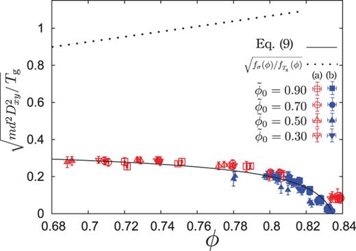
The numerical data for |$\sqrt {md^2 D_{xy} / T_{\mathrm {g}}}$| with Eq. (9) are compared for |$\phi < \phi _{\rm s}$|⁠. The deviated data exist around |$\phi \simeq 0.84$| in the (a) layer, which may result from the existence of the source point at |$y \simeq 0$|⁠. We also plot |$\sqrt {f_{\sigma }(\phi)/f_{T_{\mathrm {g}}}(\phi)}$| as the dashed line for comparison.

Open in new tabDownload slide

However, there exists the inhomogeneity of |$T_{\mathrm {g}}$|⁠, as in the dead zone near the target. This is because we can generalize the discussion of Bagnold's scaling, at least if the inhomogeneity is small (see Appendix B). Indeed, our case satisfies the condition that the gradient of the thermal velocity |$\sqrt {2T_{\mathrm {g}}/m}$| is much smaller than that of the velocity field, because the momentum transfer plays major roles in the energy balance equation, where the only relevant time scale would be the shear rate. The detailed analysis for the inhomogeneity of |$T_{\mathrm {g}}$| is shown in Appendix B.

3.4 Constitutive equation

3.4.1 Effective friction constant

Fig. 6.

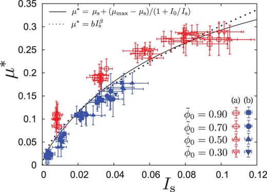
Numerical data for the bi-dispersed frictionless grains are plotted on the |$\mu ^*$| vs |$I_{\mathrm {s}}$| plane. Red and blue points denote data for the (a) and (b) layers for several |$\tilde {\phi }_0$|⁠, respectively. All points are fitted into the phenomenological equation in Eqs. (14) and (15), where we cannot judge which equation is better from the data.

Open in new tabDownload slide

3.4.2 The asymptotic divergence of the shear stress

Fig. 7.

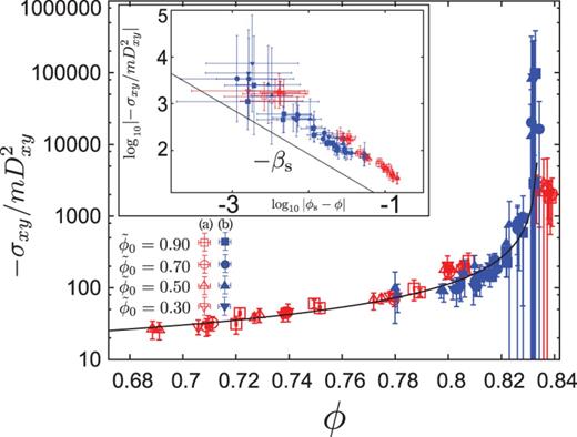
Equation (17), which denotes the divergence of the shear stress, is independently checked for the bi-disperse frictionless case. Red and blue points denote data for the (a) and (b) layers for several |$\tilde {\phi }_0$|⁠, respectively. Equation (17) reproduces the numerical results well. Because |$\sigma _{xy}$| itself in the (b) layer are small, the error bars in the (b) layer are larger than those in the (a) layer. In the inset, we plot |$\log _{10} |-\sigma _{xy}/mD_{xy}^2|$| vs |$\log _{10} |\phi _{\mathrm {s}} - \phi |$|⁠, to examine how good Eq. (17) is.

Open in new tabDownload slide

Let us compare our observed critical behavior of the shear stress with the case of the jamming transitions, in detail as well as through extrapolation of the kinetic theory. When we adopt the extrapolation of the kinetic theory, we have |$-\sigma _{xy}/mD_{xy} ^2 = \eta /mD_{xy} \sim \eta ^* \sim \phi ^2 g(\phi) \sim \phi _c ^2/(\phi _c - \phi)$| as |$\phi \to \phi _c$|⁠, i.e. |$\beta _{\mathrm {s}} = 1.0$|⁠, where |$T_{\mathrm {g}} \sim md^2 D_{xy}^2$| is used and dimensionless shear viscosity |$\eta ^* \equiv \eta / \eta _0$| is introduced with |$\eta _0 \equiv \sqrt {m T_{\mathrm {g}} /4\pi d^2}$| and shear viscosity |$\eta \equiv - \sigma _{xy} / D_{xy}$|⁠. The extrapolation from the kinetic regime by Garcia-Rojo et al. predicts that |$\sigma _{xy}$| diverges at a density different from |$Pd^2/T_{\mathrm {g}}$| and |$\beta _{\mathrm {s}} = 1.0$| [49]. Therefore, our analysis based on the power-law friction Eq. (15) predicts results similar to Garcia-Rojo et al. [49]: |$\beta _{\mathrm {s}} = 1.0$| and |$\phi _{\mathrm {s}} < \phi _{\mathrm { T}}$|⁠. On the other hand, the exponents for the divergence of |$-\sigma _{xy}/mD_{xy}^2$| at the jamming transition for sheared granular materials are estimated to be |$\beta _{\mathrm {s}} \simeq 2.6$| from data in Ref. [48] and |$\beta _{\mathrm {s}} = 4.0$| in Ref. [44]. Thus, our corresponding exponent |$\beta _{\mathrm {s}} = 0.96$| is much smaller than those of the jamming transition for sheared granular systems and rather close to the result of the kinetic theory. Otsuki et al. [44] studied the difference of soft core jamming and the asymptotic divergence of hard core systems. Then, they confirmed that the exponent |$\beta _{\mathrm {s}}$| can only deviate from 1.0 in a very narrow critical region, in which the soft core effect becomes relevant. Although our system has high density, the number of particles in contacts is still not large. Therefore, we may regard the granular fluid after the impact as a hard core fluid.

4. Effect of the friction constant

We examine how the fluid state depends on the friction constant from the simulation for |$\mu _{\mathrm {p}} = 0.2$|⁠, |$0.4$|⁠, and |$1.0$|⁠. It is noteworthy that the separation between the (a) and (b) layers exists for larger |$\mu _{\rm p}$|⁠, even on the |$\phi $| vs |$I_{\mathrm {s}}$| plane. The results for |$\mu _{\mathrm {p}} = 0.2$| and |$\mu _{\mathrm {p}} = 1.0$| are shown in Fig. 8 (i) and (ii), respectively. Because there are two branches on the |$\phi $| vs |$I_{\mathrm {s}}$| plane, we adopt Eq. (3) to fit the data in the (a) or (b) layer, separately. Figure 9 shows the critical densities and the exponents for each |$\mu _{\mathrm {p}}$|⁠, where |$\phi _{\rm s}$| in both (a) and (b) layers slightly decreases as |$\mu _{\mathrm {p}}$| increases, and |$\alpha _{\mathrm {s}}$| in the (a) layer increases as |$\mu _{\mathrm {p}}$| increases, while it decreases in the (b) layer. We note that the decreases of our critical densities |$\phi _{\mathrm {s}}$| in both the (a) and (b) layers are gentler than the |$\phi _{\mathrm {L}}$| of the jamming transition for sheared granular systems [39].

Fig. 8.

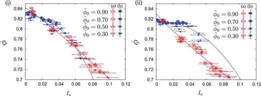
Fitting results of Eq. (3) for |$\mu _{\mathrm {p}} = 0.2$| (i) and |$\mu _{\mathrm {p}} = 1.0$| (ii). As |$\mu _{\mathrm {p}}$| becomes larger, data for the (a) and (b) layers deviate from each other.

Open in new tabDownload slide

Fig. 9.

The |$\mu _{\mathrm {p}}$| dependence of the critical density |$\phi _{\mathrm {s}}$| and the exponent |$\alpha _{\mathrm {s}}$| in (i) and (ii), respectively. |$\phi _{\mathrm {s}}$| in both (a) and (b) layers slightly decreases as |$\mu _{\mathrm {p}}$| increases. The purple solid line denotes the corresponding critical density of jamming for frictional granular particles |$\phi _{\mathrm {L}}$| [39]. The exponents in the (a) layer increase as |$\mu _{\mathrm {p}}$| increases, while they decrease in the (b) layer.

Open in new tabDownload slide

In contrast, the friction law is little affected by the friction of grains. The results for the friction law are shown in Fig. 10 (i) for |$\mu _{\mathrm {p}} = 0.2$| and (ii) for |$\mu _{\mathrm {p}} = 1.0$|⁠, where the numerical data can be fitted by both Eqs. (14) and (15). We stress that |$\mu ^*$| monotonically increases from near zero as |$I_{\mathrm {s}}$| increases, even for large |$\mu _{\mathrm {p}}$|⁠.

Fig. 10.

Numerical data for |$\mu _{\mathrm {p}} = 0.2$| (i) and |$\mu _{\mathrm {p}} = 1.0$| (ii) can be fitted into Eqs. (14) and (15) within error bars, where we cannot judge which equations are better. The friction law is little affected by the friction of grains. It should be noted that |$\mu ^*$| monotonically increases from near zero as |$I_{\mathrm {s}}$| increases, even for large |$\mu _{\rm p}$|⁠.

Open in new tabDownload slide

5. Result for the mono-disperse case

Here, we discuss the impact of granular jets in 2D for the mono-disperse case. A typical snapshot zoomed near the target is shown in Fig. 11, where grains are crystalized near the wall. The black solid lines in Fig. 11(i) are drawn by hand to clarify the grain boundary between the crystallized region and the disordered region, where the boundary becomes a slip line. We also visualize all of the corresponding contact force network in Fig. 11(ii).

Fig. 11.

Typical snapshot of the simulation for the frictionless and mono-disperse grains case with |$\tilde {\phi }_0 = 0.90$| near the target. Green particles denote mobile grains in the granular jet and red particles are wall particles (i). The black solid lines are drawn by hand to clarify the grain boundary between the crystallized region and the disordered region, where the boundary becomes a slip line. Crystallization into a triangular lattice can be seen near the region enclosed by the black lines. All of the corresponding contact forces between grains are visualized as black-colored arrows in (ii).

Open in new tabDownload slide

The notable difference in the mono-disperse cases from the bi-disperse cases appears in the friction law. We plot |$\mu ^* (I_{\mathrm {s}})$| for the mono-disperse case of frictionless grains, |$\mu _{\mathrm {p}} = 0.2$|⁠, and |$\mu _{\mathrm {p}} = 1.0$| in Fig. 12 (i), (ii), and (iii), respectively. First of all, |$\mu ^* (I_{\mathrm {s}})$| for both (a) and (b) layers cannot be fitted by a single curve, unlike the bi-disperse case. Judging from the snapshot (Fig. 11), grains, at least in the (a) layer, are partially crystallized. Therefore, it is reasonable that the response of the crystallized region is different from that in disordered regions in the (b) layer.

Fig. 12.

Numerical data for the frictionless case (i), |$\mu _{\mathrm {p}} = 0.2$| (ii), and |$\mu _{\mathrm {p}} = 1.0$| (iii) are plotted on the |$\mu ^*$| vs |$I_{\mathrm {s}}$| plane. Red and blue points denote data for the (a) and (b) layers for several |$\tilde {\phi }_0$|⁠, respectively. Unlike the bi-disperse cases, |$\mu ^* (I_{\mathrm {s}})$| for (a) and (b) cannot be fitted into a single curve. |$\mu ^* (I_{\mathrm {s}})$| in (i)–(iii) show similar behavior in the (a) layer. However, in the (b) layer, because frictionless grains cannot roll over the crystallized region, |$\mu ^* (I_{\mathrm {s}})$| for the frictionless case shows a similar dependence on |$I_{\mathrm {s}}$| to that in the (a) layer, while the corresponding |$\mu ^* (I_{\mathrm {s}})$| for frictional cases do not.

Open in new tabDownload slide

The behavior of |$\mu ^* (I_{\mathrm {s}})$| in the (a) layer in both frictional and frictionless cases can be understood as follows. Because of the crystallization, a grain is trapped in a crystallized region. However, as |$I_{\mathrm {s}}$| increases, the grain can escape from the crystallized region. Thus, |$\mu ^*$| decreases as |$I_{\mathrm {s}}$| increases.

The macroscopic friction |$\mu ^*(I_{\mathrm {s}})$| for frictionless grains is different from that for frictional grains in the (b) layer. The most remarkable difference between the frictionless and the frictional cases is the existence of a peak of |$\mu ^*$| at a small |$I_{\mathrm {s}}$| for the frictionless case, while there is no such peak for frictional cases. Because a frictional grain can roll over grains, grains easily form a cluster. Therefore, the boundary between such clusters becomes a slip line. Thus, |$\mu ^* (I_{\mathrm {s}})$| would be constant as |$I_{\mathrm {s}}$| becomes smaller. On the other hand, because a frictionless grain can neither roll over them nor slip, it is trapped in the crystallized region even for large |$I_{\mathrm {s}}$|⁠. Thus, |$\mu ^*(I_{\mathrm {s}})$| for the frictional and frictionless cases exhibit different behaviors in the (b) layer. However, we should stress that there exist two metastable branches for both frictionless and frictional cases.

6. Discussion and Conclusion

We have performed two-dimensional simulations for the impact of a granular jet and discussed its rheology. We confirmed the existence of the dead zone, as is reported in Ref. [15], at least in the (a) layer, unlike our previous three-dimensional cases [12,13]. There exists large normal stress difference, which has not been reported previously. The shear stress is much smaller than the normal stress, at least in the (b) layer. We need to solve the inconsistency in the (a) layer with Ref. [15].

We have analyzed the rheology of frictionless grains after the jet impact. We found that the pressure and the shear stress diverge with exponents similar to the extrapolations from the kinetic regime, and their exponents are smaller than those of the jamming transition for sheared granular systems. We adopted the power-law friction for |$\mu ^*$|⁠, Eq. (15), to obtain the critical exponent for |$\sigma _{xy}/mD_{xy}^2$|⁠. The discrepancy between our case and the jamming transition for sheared granular systems originates from: (i) our system cannot reach the true jamming transition, and (ii) the uncontrollability of |$D_{xy}$| in our setup. The jamming point for a sheared system |$\phi _{\mathrm {J}}$| is located between |$\phi _{\mathrm {s}} < \phi _{\mathrm { J}} < \phi _{\mathrm { T}}$| and is close to |$\phi _{\rm s}$|⁠. Our analysis based on the power-law friction is consistent with that by Garcia-Rojo et al. [49], where |$\sigma _{xy}$| diverges at a density different from |$Pd^2/T_{\mathrm {g}}$| [49].

The effects of the friction of grains |$\mu _{\mathrm {p}}$| have been discussed. Although Guttenberg [14] suggested that |$\mu _{\mathrm {p}}$| does not play a significant role, at least in the scattering angle via the approximate hard sphere method [58], we found that the existence of the friction affects the rheology of granular fluids after the impact. The separation between the (a) and (b) layers appears for larger |$\mu _{\mathrm {p}}$|⁠, even on the |$\phi $| vs |$I_{\mathrm {s}}$| plane. The critical fraction |$\phi _{\mathrm {s}}$| decreases as |$\mu _{\mathrm {p}}$| increases, which is similar to the behavior of the critical fraction of jammed frictional grains |$\phi _{\mathrm {L}}$|⁠. The corresponding exponent |$\alpha _{\mathrm {s}}$| increases (decreases) as |$\mu _{\mathrm {p}}$| increases in the (a) layer ((b) layer).

The effective friction constant |$\mu ^* (I_{\mathrm {s}})$| for the mono-disperse case has two branches because of the coexistence of the crystallized state and a liquid state. On the other hand, |$\mu ^* (I_{\mathrm {s}})$| for the bi-disperse case can be described by known constitutive equations for dense granular flow [30–37].

Finally, let us comment on the rheological model proposed in a recent paper of the Chicago group [17]. It is suggested that the granular fluid after the impact may be described by the plastic flow without the viscous stress and with the isotropic pressure. This suggestion is interesting, but our data may not support their suggestion. In fact, our data suggest the existence of the viscous term (the shear stress depends on the location), the pressure is anisotropic, and no evidence of the existence of the residual stress, as is shown in Fig. 6.

Acknowledgements

We thank M. Otsuki for valuable discussions. A part of the numerical computation in this work was carried out at the Yukawa Institute Computer Facility. This work is partially supported by the Grant-in-Aid for the Global COE program “The Next Generation of Physics, Spun from Universality and Emergence” from MEXT, Japan and Grant-in-Aid for Scientific Research from MEXT (No. 25287098).

Appendix A. On artificial burst-like flows for the large |$\mu _{\mathrm {p}}$| case

In this appendix, we comment on the artificial burst-like flow in 2D, which appears in the case of large |$\mu _{\rm p}$| with softer grains than those in the text. After the impact of a jet composed of softer grains with large |$\mu _{\mathrm {p}}$|⁠, the burst occurs when a grain slips, because a large tangential force can be accumulated before the slip of a grain. In Fig. 13, we show the time evolutions of |$T_{\mathrm {g}}$| at |$-\Delta y<y<0$| in the (a) layer for (i) the frictionless case and |$\mu _{\mathrm {p}} = 0.2$|⁠, and (ii) |$\mu _{\mathrm {p}} = 1.0$| with several stiffnesses, where |$T_{\mathrm {g}}$| for the frictionless case and |$\mu _{\mathrm {p}} = 0.2$| reaches small steady values, while |$T_{\mathrm {g}}$| increases many times after the impact for |$\mu _{\mathrm {p}} = 1.0$| with large |$t_{\mathrm {c}}$|⁠, due to the slip events. As |$t_{\mathrm {c}}$| becomes smaller, the burst-like flows are suppressed. Thus, we use harder grains for large |$\mu _{\mathrm {p}}$|⁠. Though there are a few small raises of |$T_{\mathrm {g}}$| for the frictionless case, they are out of our averaging time.

Fig. 13.

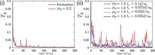
The time evolution of |$T_{\mathrm {g}}$| at |$-\Delta y<y<0$| in the (a) layer for the frictionless and |$\mu _{\mathrm {p}} = 0.2$| cases (i) and |$\mu _{\mathrm {p}} = 1.0$| for several stiffnesses of grains (ii). As |$t_{\mathrm {c}}$| becomes smaller, i.e. as grains become stiffer, the burst-like flows are suppressed.

Open in new tabDownload slide

Appendix B. Inhomogeneity of |$T_{\mathrm {g}}$|

Here, let us discuss the effect of the inhomogeneity of |$T_{\mathrm {g}}$| on Bagnold's scaling. We demonstrate that |$T_{\mathrm {g}} \sim md^2D_{xy}^2$| may be valid because the gradient of |$\sqrt {2T_{\mathrm {g}}/m}$| is much smaller than that of the velocity field in our setup.

The numerical data for the profiles of |$\sqrt {2T_{\rm g}/m}$|⁠, |$\bar {v}_{x}$|⁠, and |$|\bar {v}_{y}|$| are shown in Fig. 14 (i) and (ii). Red empty (i) and blue filled (ii) points denote the data in the (a) and (b) layers, respectively. The corresponding triangle, square, and circle points are the data for |$\sqrt {2T_{\mathrm {g}}/m}$|⁠, |$\bar {v}_x$|⁠, and |$|\bar {v}_y|$|⁠, respectively in Fig. 14. Although |$\sqrt {2T_{\mathrm {g}}/m}$| is smallest at the center |$y \simeq 0$| in the (a) layer, the inhomogeneity of |$T_{\mathrm {g}}$| is much smaller than that of |$\bar {v}_x$| and |$|\bar {v}_y|$|⁠. In particular, it is notable that |$|v_y|$| linearly increases as |$|y| \to R_{\mathrm {tar}}$| from zero.

Fig. 14.

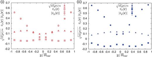
Red empty (i) and blue filled (ii) points denote the data in the (a) and (b) layers, respectively. The corresponding triangle, square, and circle points are the data for |$\sqrt {2T_{\mathrm {g}}/m}$|⁠, |$\bar {v}_x$|⁠, and |$|\bar {v}_y|$|⁠, respectively. Although |$\sqrt {2T_{\rm g}/m}$| is smallest at the center |$y \simeq 0$| in the (a) layer, the inhomogeneity of |$T_{\mathrm {g}}$| is smaller than that of |$\bar {v}_x$| and |$|\bar {v}_y|$|⁠. |$|v_y|$| linearly increases as |$y \to R_{\mathrm {tar}}$| from zero.

Open in new tabDownload slide

Fig. 15.

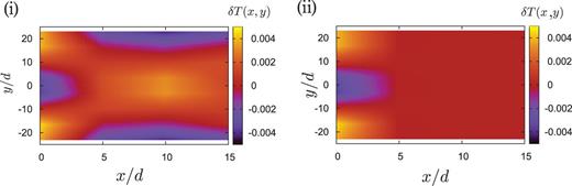
Comparison between simulation data (i) and Eq. (B13) (ii). The inhomogeneity of |$\delta T$| appearing in the dead zone rapidly decreases as |$x \to \infty $|⁠. The characteristic length for the inhomogeneity is calculated to be |$1/kd \simeq 0.696 < \Delta x$|⁠.

Open in new tabDownload slide

References