


Abstract
A conservation law along with stability, recovering phenomena, and characteristic patterns of a nonlinear dynamical system have been studied and applied to physical, biological, and ecological systems. In our previous study, we proposed a system of symmetric 2n-dimensional conserved nonlinear differential equations. In this paper, competitive systems described by a 2-dimensional nonlinear dynamical (ND) model with external perturbations are applied to population cycles and recovering phenomena of systems from microbes to mammals. The famous 10-year cycle of population density of Canadian lynx and snowshoe hare is numerically analyzed. We find that a nonlinear dynamical system with a conservation law is stable and generates a characteristic rhythm (cycle) of population density, which we call the standard rhythm of a nonlinear dynamical system. The stability and restoration phenomena are strongly related to a conservation law and the balance of a system. The standard rhythm of population density is a manifestation of the survival of the fittest to the balance of a nonlinear dynamical system.
1. Introduction
The concept of stability is important in order to understand natural phenomena in physical, biological, and engineering systems. In our previous study, we studied the relation between a conservation law and the stability of a 2n-dimensional competitive system that contains competitive interactions, self-interactions, and mixing interactions. The system consists of 2n-dimensional nonlinear differential equations required from Noether's theorem [1]. The 2n-dimensional nonlinear ordinary differential equations for a competitive system constructed to satisfy the conservation law have properties such as the addition law, which is empirically interpreted as recovery from injuries of skin and tissues in biological bodies.
It has been shown by many researchers that a relatively simple set of interactions can explain complex phenomena in biological systems [2,3]. For example, in 1952, Turing suggested a chemical molecular mechanism called the reaction–diffusion system [4] which is defined as semi-linear parabolic partial differential equations. This reaction–diffusion system is well applied in explaining the stripe patterns of the marine angelfish, Pomacanthus, and restoration phenomena in its stripe patterns from injuries was observed [5–7]. Prigogine also proposed the Brusselator model with nonlinear ordinary differential equations to illustrate spatial oscillations and Turing patterns [8]. It is also an interesting problem to investigate for ecological systems whether a large complex system should be stable or not, and many researchers have discussed the criteria concerning the stability of systems of n-dimensional ordinary differential equations in statistical frameworks and mechanics [9–15]. What would be the reason for a simple set of interactions to explain complex phenomena? We discussed a system of interactions generalizing Lotka–Volterra-type nonlinear competitive interactions and suggested that a conservation law could be a key to understanding complex phenomena even in biological and ecological systems.
We investigated the system of 2n-dimensional coupled first-order differential equations by using Noether's theorem, which led to the following results. (i) The form of the differential equations and coefficients of nonlinear interactions are strictly confined when the system has a conservation law which is constructed by interacting species of a particular experimental system. (ii) The conserved quantity of a system produces a Lyapunov function which is usually employed to study solutions of nonlinear differential equations. The conserved quantity is constructed by Noether's theorem, but the analysis of the Lyapunov function would be used to check solutions to differential equations, including those for non-conservative and dissipative systems. The system of differential equations with conservation law is different in this respect. (iii) A system of interactions could be analyzed as an assembly of a basic binary-coupled form (BCF). In other words, a complex interacting system can be decomposed into an assembly of binary-coupled systems. The BCF system is a simple basic set to explain complex phenomena defined by Noether's theorem. (iv) The BCF system with conservation law indicates an addition law which may be interpreted as the restoration or rehabilitation phenomenon; these are known in large systems such as neural networks or computer networks when a small disordered device or part of the network system is replaced by a normal device. These properties could be applied to stability and restoration phenomena of biological systems. (v) The conservation law is also useful in checking the accuracy of numerical solutions to nonlinear differential equations. As summarized above, we discussed that the basic nonlinear system in BCF is stable. The binary-coupled system and addition law supported by a conservation law can lead to a large, stable, complex system. This is an important conclusion on the conserved binary-coupled model. Because the BCF system has such interesting properties, we will apply the model in order to study stability and interaction mechanisms of biological systems.
In this paper, we will explain the properties of solutions with a conservation law and applications to biological systems. In Sect. 2, we extend the BCF model to simulate external perturbations numerically. There are various prey–predator-type competitive models with perturbations; however, most of them are with small, stochastic perturbations. The behaviors of conservation laws with external perturbations have seldom been considered. We will explicitly discuss properties of the conserved, stable, 2-variable nonlinear interacting system with external perturbations and the conservation law, its indications and possible applications to nonlinear interacting systems. We will show that the 2-variable ND model has the properties of restoration and recovery from external perturbations. In Sect. 3, stability and population cycles of biological systems are examined in terms of a conservation law of the system. We will also examine the specific examples of the Canadian lynx and snowshoe hare [16–22] and the question of population cycles, and the food chain of microbes in a lake [23,24]. Conclusions and summary of results are given in Sect. 4.
2. The model of binary-coupled form (BCF)
2.1 2n-ND system with perturbations
The physical meaning of conserved quantities in a biological system is difficult to define, contrary to classical mechanics in physics, and so we would like to explain the differences between the Ψ-function and the Hamiltonian. The Ψ-function in this study is derived from Noether's theorem with Euler–Lagrange equations of motion applied to the 2n-ND system. We discussed the binary-coupled form to generalize a Lotka–Volterra-type competitive system in the previous work.
The binary-coupled system has the conserved quantity (Ψ-function), and the Ψ-function may have similar physical meanings as the Hamiltonian of a system. However, the Hamiltonian is defined as the total energy of a system, and the energy has the dimension of work, which is defined as force |$\times $| displacement [25,26]. The conserved quantity Ψ is constant with time, but it is constructed from interactions of a 2n-ND system, not from the force, kinetic energy, and potentials which are, in principle, converted to the work produced by the system. Hence, the Ψ-function may well be called the “conserved quantity,” but not the Hamiltonian of the system. The Ψ-function may correspond to (generalized) kinetic and potential energies of a system, but it is not possible to prove that the Ψ-function is equivalent to the Hamiltonian in terms of physics. In the 2n-ND model, variables denote population densities of a system of extended Lotka–Volterra-type differential equations, and it is inappropriate to directly interpret the Ψ-function as the total energy or biomass of the system. However, it is important to comprehend that the conserved Ψ-function controls behaviors and properties of the system.
We showed that the conserved quantity, the Ψ-function, can reproduce the Lyapunov function of classical Lotka–Volterra equations in the previous work [1]. It is essential to understand that Lyapunov functions for certain systems of differential equations can be derived from Noether's theorem when a system has conserved quantities. Hence, in conserved systems such as 2n-ND systems, the conservation law and Noether's theorem are fundamental to studying properties of the system. The system with the Lyapunov function has limit cycles and attractors, which designate energy dissipations of the system. The dynamics of the system of the Ψ-function evolves according to the conservation law Ψ, and hence there are no energy dissipations, which is equivalent to Lagrangian dynamics in physical systems.
2.2 Properties of a 2-variable ND model
The nonlinear interactions can generally represent, for example, Lotka–Volterra-type prey–predator, competitive interactions, or food-chain relations by adjusting nonlinear parameters |$\alpha _1, \dots , \alpha _8$| (see Table 1). The piecewise continuous constants |$c_1$| and |$c_2$| are used as external perturbations in computer simulations, such as environmental conditions which increase or decrease the interacting species in question. Equations (4)–(6) form 2-variable BCF nonlinear differential equations with a conservation law.
The list of nonlinear coefficients.
| α1 | α2 | α3 | α4 | α5 | α6 | α7 | α8 | |
|---|---|---|---|---|---|---|---|---|
| Condition 1 | 1.0 | 401.0 | −0.35 | 1.5 | 10.5 | −0.01 | −0.006 | −0.011 |
| Condition 2 | 1.0 | 401.0 | −0.35 | 1.5 | 10.5 | −0.51 | −0.006 | −0.011 |
| α1 | α2 | α3 | α4 | α5 | α6 | α7 | α8 | |
|---|---|---|---|---|---|---|---|---|
| Condition 1 | 1.0 | 401.0 | −0.35 | 1.5 | 10.5 | −0.01 | −0.006 | −0.011 |
| Condition 2 | 1.0 | 401.0 | −0.35 | 1.5 | 10.5 | −0.51 | −0.006 | −0.011 |
By employing Eqs. (4)–(6), we will show:
Solutions to the binary-coupled nonlinear equations maintain a characteristic |$(x_1,x_2)$| phase-space of solutions and recovery from external perturbations. The external perturbations can numerically reproduce environmental conditions such as temperature, climate, and chemical substances which affect interacting species. The nonlinear binary-coupled model can be applied to examine responses of a system whether they are induced from internal interactions or external perturbations.
The binary-coupled nonlinear equations with conservation law exhibit stable phase-space solutions, which are interpreted as stability and recovery of population change in a biological system. The properties of the binary-coupled nonlinear interactions will be shown explicitly in numerical simulations.
By employing the 2-variable binary-coupled model, it is possible to simulate cycles of maxima and minima in population change, and delays of periodic times of population cycles for competitive species. Hence, cycles of population change will be discussed in terms of the conservation law and nonlinear interactions.
Figure 1(a) shows the nonlinear interactions between species without external perturbations (|$c_1=0$| and |$c_2=0$|), whose coefficients of nonlinear equations are set as in Table 1 (Condition 1). In the classical Lotka–Volterra competitive system, this can be interpreted as that |$x_1$| and |$x_2$| represent prey and predator, respectively. Figure 1(b) is the phase-space given by solutions |$(x_1, x_2)$|. The solutions |$(x_1, x_2)$| are periodic with respect to time, the maxima and minima of |$(x_1, x_2)$| appear with a time delay. Figure 1(c) shows the numerical value of the conserved function Ψ defined by (6), which is constant with respect to time.
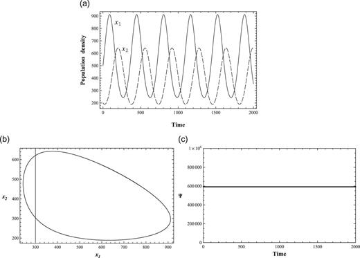
A 2-variable ND solution and conservation law Ψ. (a) 2-variable ND solutions. Solid and dashed lines represent |$x_1$| (prey) and |$x_2$| (predator), respectively. One should note that the unit of time should be defined with respect to the system in consideration, (b) Phase-space of 2-variable ND solutions, and (c) Conservation law Ψ of 2-variable ND. It is constant with respect to time.
The solutions |$(x_1, x_2)$| in Fig. 1(a) show explicitly a time delay of the peak for interacting species. The timings of peak and delayed peak are determined by nonlinear interactions and the strength of the coupling constant. The solutions |$(x_1, x_2)$| in Fig. 1(b) show phase-space solutions, which are stable in the sense that the conserved quantity Ψ is maintained constant and phase-space solutions are in the same trajectory for all time. The unit of time should be considered to adjust to the time scale of a system in consideration, because biological unit times are generally different from microbes to mammals.
The phase-space diagram Fig. 1(b) and the straight line of Fig. 1(c) show that the solution is exact and stable [1]. The three figures exhibit important properties of solutions to systems of prey–predator-type competitive nonlinear interactions. Because of the positivity |$x_i \geq 0$|, the nonlinearity and the conservation law Ψ, the values of the coupling constants in the 2n-ND equations are strongly restricted to generate meaningful solutions, which indicates that initial values and coupling constants, among others, are strongly interrelated. Therefore, it is difficult to generate admissible solutions by finding combinations of coupling constants and perturbations maintaining the constancy of Ψ. One should note that admissible solutions of an ND system with conservation law cannot simply and continuously depend on initial population densities and coupling constants as well as the condition of conservation law Ψ; an example will be discussed in Sect. 2.3.
One of the important properties shown by the stable, conserved nonlinear system is that the interacting species repeat the rhythm of population maxima and minima. The periods of the rhythm are the result of complicated nonlinear interactions, but the system keeps the quantity Ψ constant with respect to time. The interesting applications of the BCF model are shown by employing “Mysis in the Okanagan Lake food web” [23], and in Canadian lynx and snowshoe hare [17], which will be explained in Sect. 3.
2.3 Recovering and restoration from perturbations
Figures 2(a), 2(b), and 2(c) show the reaction and recovery of the nonlinear interacting system from an external perturbation. One of the typical recoveries of a system from a perturbed state is shown. In Fig. 2(a), an external perturbation starts at |$t=700$| (Sp. 1); the coefficient |$f_1$| equals −1260.0 and |$f_2$| equals zero in this example. The black arrow is the starting point of the perturbation, and the gray arrow is the end of the perturbation in Figs. 2(a) and 2(c). The nonlinear coefficients are listed in Table 1 (Condition 1). The solutions |$(x_1,x_2)$| are deformed by the perturbation (Figs. 2(a) and 2(b)). However, the system does not disintegrate but finds a new stable phase-space close to the original phase-space and maintains a new conserved relation. The perturbation ends at |$t=1200$| (Ep. 1), and the system recovers the original state |$(x_1,x_2)$|.
We have checked that if the perturbation and duration times are small compared to the periodic time and amplitude of species |$(x_1,x_2)$|, the system could be stable. The strengths of external perturbations are assumed and introduced as constants, and the maximum value of the constants or threshold are evaluated numerically. It is difficult to choose appropriate magnitude and duration times for perturbations, because the nonlinearity is so intense that the interrelation between coupling constants and perturbations is involved.
The timing of a negative perturbation which reduces the population number |$x_1$| or |$x_2$| produces different results. When a negative perturbation is exerted in the increasing phase of |$x_1$| or |$x_2$|, the system will find a new conserved stable solution near the original solution, but when a strong negative perturbation is exerted before |$x_1$| or |$x_2$| gets to its minimum, the system may collapse: the system exhibits no solutions |$(x_1, x_2)$|, which would be interpreted as disintegration or extinction in biological systems.
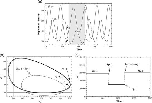
An external perturbation and a recovery. (a) 2-variable ND solutions with a negative perturbation on prey |$x_1$|. The perturbation is introduced from |$t = 700$| to |$t = 1200$|, which is represented as gray background, (b) The |$(x_1,x_2)$| phase-space transition with the negative perturbation as in (a). The solid line (St. 1) is the initial state, and St. 2 is the recovered state after the end of perturbation. The dashed line is the phase-space during Sp. 1–Ep. 1, and (c) Conservation law Ψ of 2-variable ND with one perturbation. Ψ changed from |$\Psi \simeq 60000$| to |$\Psi \simeq 30000$| by introducing the perturbation. It recovers after Ep. 1.
The conserved nonlinear system naturally exhibits maxima and minima without external perturbations; we call these endogenous maxima and minima. This is needed to distinguish them from the enhanced maxima and minima as a result of external perturbations.
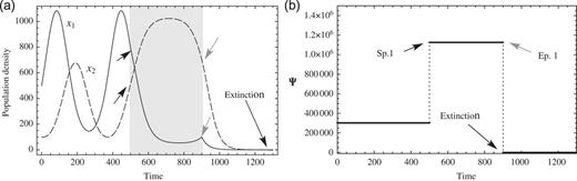
In Fig. 3, the response to a strong negative perturbation to prey after the peak of the endogenous maximum is shown. The values of the coefficients are listed in Table 1 (Condition 1). The starting point of this perturbation is at |$t=800$| and the end point of the perturbation is at |$t=950$|. The negative constant of perturbation is |$f_1=-3175.3879$|. The prey, |$x_1$|, rapidly declines with the negative perturbation, and (|$x_1$|, |$x_2$|) converges to zero for |$t \gtrsim 1000$|. These computer simulations may be compatible with known empirical results, for example, in pest control. Pest control is not so effective if it is performed in the season when harmful insects are at a peak and active, because species are energetic enough to find a new stable life to live. It is effective when performed in the season when harmful insects are not so active or in a declining state after an endogenous maximum.
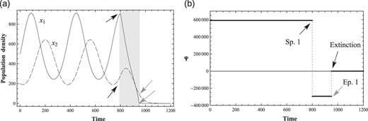
Critical negative perturbation and extinction. (a) 2-variable ND solutions with a critical negative perturbation on prey |$x_1$|. Solutions converge to zero after the perturbation and (b) Conservation law Ψ with a critical negative perturbation. Ψ converges to zero after the critical perturbation.
In the nonlinear interacting system, positive perturbations which will increase |$x_1$| or |$x_2$| do not always mean a positive effect on the stability of the system. There is a limit to the value of a positive perturbation, because an increase of |$x_1$| leads to a decrease of |$x_2$| in a stable system |$(x_1, x_2)$|, which indicates that a system has internally allowed maximum and minimum populations.
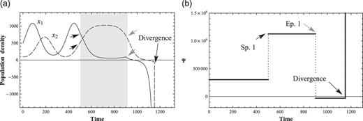
Figure 4 shows the behaviors of |$(x_1, x_2)$| at normal and critical values of positive perturbations, |$c_1$|, for |$x_1$|. The values of the coefficients are listed in Table 1 (Condition 2). Figures 4(a) and 4(b) show that the normal positive perturbation which increases the interacting species will increase the peak of the |$(x_1, x_2)$| populations. However, at certain critical values of the coupling constants, the prey–predator interaction cannot support the rhythm of maxima and minima, and the system diverges. Figures 4(c) and 4(d) show that the system cannot maintain a stable, interacting system when the positive perturbation surpasses the critical value (|$c_1=1599.924999$| in the current simulation). The unstable solutions branch out at |$t \simeq 1100$| when the value of perturbation changes from |$f_1=1160.0$| to |$f_1=1599.924999$|.
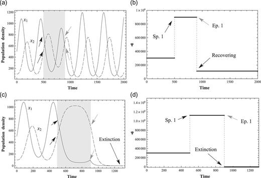
Critical perturbations and divergence of solutions. (a) 2-variable ND solutions with a positive perturbation. The perturbation starts at |$t = 500$| and ends at |$t = 900$|, represented as a gray background. The amplitudes of |$x_1$| and |$x_2$| become larger than before, (b) The conserved quantity Ψ with a positive perturbation. It recovers after perturbation but finds another equilibrium state, (c) 2-variable ND solutions with a critical perturbation. |$x_1$| and |$x_2$| converge to zero after a critical perturbation, and (d) Conservation law of 2-variable ND with a critical perturbation. Ψ converges to zero after a critical perturbation.
The solutions of |$(x_1,x_2)$| are restricted to |$x_i \geq 0$| because negative solutions are not meaningful in the analysis of this model, and this confines the values of the coupling constants |$\alpha _i$|. The coupling constants and initial values are strictly restricted by the conservation law Ψ, in order to produce positive |$x_i$|. In Figs. 3 and 4, solutions |$x_1$| and |$x_2$| are positive values. When solution |$x_1$| and |$x_2$| are less than zero, |$x_1$| and |$x_2$| are considered extinct.
The |$(x_1,x_2)$| ND system with conservation law cannot simply become negative with perturbations over the critical values. This is different from other nonlinear Lotka–Volterra-type nonlinear equations. The system will diverge and show no solutions when negative perturbations over critical values are exerted. For example, one should observe Figs. 5(a) and 5(b), which are the results of a perturbation slightly stronger than the critical value; we choose |$f_1 = 1600.924$|. One can see from Fig. 5 that |$x_1$| and |$x_2$| do not simply become negative and positive solutions. It shows no solutions in this conserved nonlinear model. This is a different property compared to other Lotka–Volterra equations without a conservation law.
The divergence of solutions with a perturbation over a critical value. (a) 2-variable ND solutions with a perturbation over the critical value on prey, |$x_1$|. The solutions diverge with a perturbation over the critical value and (b) Conservation law Ψ with a perturbation over the critical value. Ψ diverges with a perturbation over the critical value.
In this sense, Ψ will restrict admissible solutions consistent with nonlinear coupling constants, initial values, and perturbations in order to maintain the positivity |$x_i \geq 0$|. One should note that we consider stable solutions or systems with the assumption that |$x_1$| and |$x_2$| are positive values. We chose all solutions |$x_i$| to be positive and the coupling constants are restricted to generate physical solutions with |$x_i \geq 0$|. If one of the |$x_i$| becomes negative, the system will collapse and solutions do not exist.
The results of nonlinear interactions with a 2n-ND system with conservation law Ψ remind us of nonlinear phenomena in physics such as collective excitations, plasmons, phonons, and vibrational and rotational motions of nuclei [27]. The particles are in motion independently according to the equations of motion, but they simultaneously show collective motions as a whole, collective excitations mentioned above, which are also called cooperative phenomena.
The species interacting as prey and predator constitute a periodic phenomenon as a whole ecosystem, which looks similar to a collective phenomenon in a physical system. In this sense, we regard the phenomena of 2n-ND systems with conservation law or the prey–predator system such as the hare–lynx interactions with a periodic population change as cooperative systems.
Hence, as a nonlinear competitive and conserved stable system, species with a stable periodic change seem to show similar cooperative phenomena, collective phenomena in physics, or power laws in economical physics [28]. The nonlinear interactions with conservation law can express a stable solution supported by intricate interactions of species and environment in an ecological system.
A competitive interacting system such as the conserved prey–predator relations may be considered to be a cooperative system for species to survive. It should be noted that if a dynamical prey–predator system is active, the rhythms of maxima and minima are clearly repeated, which is known in real prey–predator systems. However, if an external perturbation (exogenous interaction) exceeds a certain critical value for the competitive system, the rhythms of maxima and minima will disappear first and then, after a time, the system will diverge (disintegrate). Therefore, the rhythm of wildlife indicates that the dynamical interactions between species are active and stable. When the rhythm of change disappears or does not come back, it may indicate that related species are in danger of extinction. The rhythm is important for evaluating whether the wildlife is normal and active, or harmed by human activities and external perturbations.
On the other hand, by adding another perturbation, we can show that it is possible to save species from extinction. Figure 6(a) is the result of a positive perturbation to save the species |$(x_1, x_2)$| in danger of extinction in Fig. 3(a). We exerted a positive perturbation after Sp. 1–Ep. 1 in Fig. 6. The positive perturbations start at |$t=1000$| (Sp. 2) and end at |$t=1300$| (Ep. 2); the strengths of |$c_1$| and |$c_2$| are |$f_1 = 200$|, |$f_2 = -1000$|. Figure 6(a) shows that the species are in danger of extinction; however, if positive external perturbations are properly inserted, the system will come back to life again.
Critical behavior and restoration. (a) 2-variable ND solutions with perturbations to avoid converging to zero after a critical perturbation. |$x_1$| and |$x_2$| come back to life after the second perturbation and (b) Conservation law Ψ with the two perturbations in (a). Ψ recovers from the perturbation after Sp. 2–Ep. 2.
Although it is difficult to consider what appropriate positive perturbations are in real ecosystems, the results of Fig. 6 indicate that executions of appropriate perturbations can save endangered species from extinction.
2.4 Comments on the “atto-fox problem”
It should be noted that a problem known as the “atto-fox problem” [29,30] in a system of differential equations will not occur in a conserved system of differential equations, because the problem is related to properties of the conserved or non-conserved system of differential equations. The 2n-ND system has the conservation law and the Ψ-function characterizes behaviors of solutions and systems. If the Ψ-function is conserved and not equal to zero (except trivial solutions), the solution will converge and the system will be stable. Nonlinear ordinary differential equations with a conservation law can have a stable solution controlled by the Ψ-function, and solutions consist of a closed hypersurface of |$(x_1,x_2,\dots ,x_{2n})$| for the 2n-dimensional case. It should be noted that the admissible coefficients of nonlinear interactions are strictly confined by the Ψ-function of the system.
The solutions to the 2n-ND equations with conservation law Ψ are different from those of other non-conserved Lotka–Volterra-type nonlinear differential equations, as shown in the example in Fig. 6; it is not possible to arbitrarily reduce a population density to very small or negative while keeping the other at a large positive value. Unphysical solutions are likely to make the Ψ-function diverge, which shows that the solutions are prohibited as shown in the example in Fig. 5.
The changes of population densities are strictly confined by the conservation law and it is not possible to change initial values, coupling constants, and the magnitude of perturbations arbitrarily in the 2n-ND equations with conservation law Ψ.
The Ψ-function will not be constant when there are no solutions or unphysical solutions, and maintaining the Ψ-function as constant will confine admissible solutions [1]. For example, if the 2-variable nonlinear interacting system has solutions which are as extremely different as |$10^{-18}$| orders, like the “atto-fox problem,” it is not possible for the system to maintain the Ψ-function as constant in time. The “atto-fox problem” is typically generated [30] in dissipative or non-conserved systems, because non-conserved systems do not have the conservation law to control admissible solutions, and a large class of (unphysical) solutions can be allowed compared to the system of the Ψ-function, which is the reason why the “atto-fox problem” could happen in non-conserved systems. Therefore, the conserved system with Ψ-function will produce physical solutions controlled by the conservation law, and a phenomenon like the “atto-fox problem” will not be allowed in a conserved system with the Ψ-function.
3. Conservation law and population cycles
3.1 The food web of microbes in Okanagan Lake
One interesting example of ecological interactions is the interaction described in “Mysis in the Okanagan Lake food web: A time-series analysis of interaction strengths in an invaded plankton community” [23]. Although the food web in Okanagan Lake is not clarified definitely, the introduction of Mysis shrimp to lakes is known as an effective method to enhance the ecological interactions and their strengths among microbes and other creatures so as to increase fisheries productions.
The time series of dominant crustacean zooplankton densities in Okanagan Lake has been measured monthly and suggested that Mysis and zooplankton populations are synchronous and characterized by the cycle of the peak and bottom population densities. The cycles of population densities are primarily due to cycles of season and climate, and then to the mutual interaction of microbes. Analysis of the microbes suggests that density-dependent and delayed population regulation of microbes is evident. In addition to the seasonal factors, the regular cycles and the delayed peak and bottom population densities of microbes are the results of strong nonlinear interactions of species. We numerically examined changes of population densities of microbes by employing the 2-variable conserved ND model.
The current conserved nonlinear model shows that the interacting species designate a standard rhythm of the peak and bottom population densities. There are some fluctuations at the peak and bottom densities, but they show stable dynamic life, as demonstrated in Fig. 7(a)–(c). Although normal peak and bottom densities can be readily explained by adjusting the coupling strength of the model's internal interactions, a sudden change of maxima which is often encountered in a biological data cannot be easily simulated by only adjusting internal coupling constants in the 2-variable nonlinear interacting model.
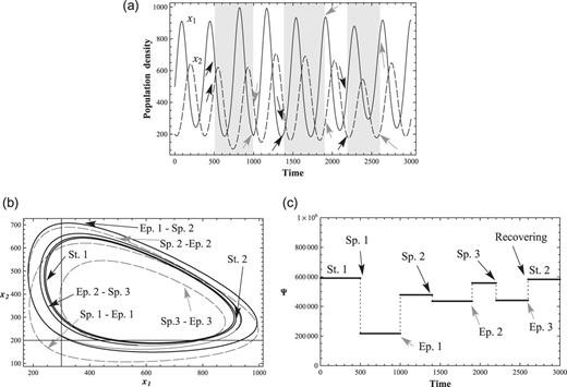
Several external perturbations and recoveries. (a) 2-variable ND solutions with three external perturbations. The rhythm of |$x_1$| and |$x_2$| recovers from several perturbations. Gray backgrounds represent periods of perturbation, (b) Phase-space transitions of |$x_1$| and |$x_2$|. Dashed lines represent solutions, |$x_1$| and |$x_2$|, during perturbations. Solid lines represent solutions without perturbations, and (c) Conservation law Ψ with three perturbations. It recovers from three perturbations. |$\Psi \simeq 60000$| in St. 1 and St. 2.
In Fig. 7, several perturbations are exerted on the interacting 2-variable system. The first external perturbation starts at |$t=500$| (Sp. 1) and ends at |$t=1000$| (Ep. 1). The strengths of the perturbations in Sp. 1–Ep. 1 are |$f_1 = -800$|, |$f_2=-100$|. The second external perturbation starts at |$t=1400$| (Sp. 2) and ends at |$t=1900$| (Ep. 2). The strengths of the perturbations in Sp. 2–Ep. 2 are |$f_1 = -50$|, |$f_2=-120$|. The third external perturbation starts at |$t=2200$| (Sp. 3) and ends at |$t=2600$| (Ep. 3). The strengths of the perturbations in Sp. 3–Ep. 3 is set as |$f_1=-500$|, |$f_2=-50$|. The lines |$(x_1,x_2)$| may represent, for instance, the prey–predator interactions, species of food chain, and species interacting with its environmental factors (temperature or some environmental effects). Black arrows are the starting points of perturbations, and gray arrows are the ends of perturbations; the parameters are listed in Table 1 (Condition 1). The time period is within |$t=4000$|; initial values are |$x_1 = 500$|, |$x_2 = 300$|.
The significant properties of the stable nonlinear conserved system are that if external perturbations are not large enough to disintegrate the system, the system will find a stable conserved solution near the original system and continue a stable cycle (maxima and minima). This is clearly seen from the |$(x_1,x_2)$| phase-space solutions in Fig. 7(b). The system recovers from several external perturbations.
Numerical analysis can be applied to examine the change of population densities of microbes. For example, the time series data of dominant crustacean zooplankton densities in Figure 2 of Ref. [23] show that the sudden maxima of dominant zooplankton densities are seen in the period ’99–’02. The sudden increase of the peak is readily adjusted when an external perturbation is assumed in the simulation; however, it is not reproduced by adjusting the internal coupling constants in the 2-variable nonlinear model. Hence, it is concluded in the 2-variable model that there would have been certain positive external perturbations to the system of microbes in Okanagan Lake during ’98–’01, considering a time delay in external perturbations.
It is interesting to check what kind of external or internal perturbations were affecting the peak of population density during the period ’98–’01. If there are no explicit changes in external or internal factors during the period, a sudden increase of the peak could be a result of more complex internal interactions. For example, the rhythm of the peak and bottom population densities should be explained by 4-variable or 6-variable nonlinear interactions of microbes. The unusual rhythm indicates how exogenous (environmental) and endogenous (internal interactions) variables are affecting the dynamics of each component and environmental nature related to the species. The analysis of the nonlinear model suggests that the sudden peak and bottom densities have important information on the dynamics of the system of species and environment. Hence, it is important to understand the standard rhythm of the peak and bottom population densities in order to distinguish them from unusual maxima and minima.
One should be careful that a positive perturbation on one of the interacting species not only enhances the peaks of maxima but also decreases minima in the rhythm of species. It is often true that the effect of enhancement is usually emphasized without taking care of later negative effects. Hence, the enhancement of the population of a specific species may be harmful to other species in the food web, and consequently it endangers itself. Our analyses in Figs. 4 and 6 show that if we carefully control the increase or decrease of the population of certain species after the introduction of a positive effect, we can keep the normal and stable dynamics of species suitable for the environment. For this purpose, it is essential to explicitly understand the standard rhythm from real observed data.
It is possible to reasonably simulate the change of populations of microbes in Okanagan Lake by employing the current conserved 2-variable ND equation, and one can refine the simulation by combining two or three sets of 2-variable ND equations for the simulation of four-microbe or six-microbe interacting systems. We expect that the current ND simulation may help analyze the changes and effects of population densities in ecosystems and we are working on 4-variable and 6-variable interaction models for the ND system, in order to apply the model to more complex problems in ecosystems.
3.2 Population regulation in Canadian lynx and snowshoe hare
It is difficult to identify population regulation mechanisms concerning the prey–predator patterns of large mammals because the large mammal's life span is relatively long compared with microbes. The prey–predator cycle for wolves and caribou takes some decades to observe; their interacting relation and behaviors have recently been revealed with modern technology (GPS-colored animals) [16]. However, the food web configuration between snowshoe hare and Canadian lynx is a well-known prey–predator-type phenomenon, and the ten-year cycle of Canadian lynx was examined from the data of Canadian lynx fur trade returns of the Northern Department of the Hudson's Bay Company (the data are from C. Elton and M. Nicholson [17]).
The Canadian lynx and snowshoe hare have a synchronous ten-year cycle in population numbers [16,18]. The fundamental mechanisms for these cycles are maintained by the important factors such as nutrient, predation, and social interactions [19]. In addition to the important factors, the nonlinear model with conservation law suggests that species of a system consequently find a strategy or a mechanism to survive for long time periods. In other words, the cycle of population density is a manifestation of the strategy or mechanism to survive, which is suggested by the stability of phase-space solutions determined by the conservation law of a system.
The nonlinear interactions with the conservation law show a standard rhythm and stability from external perturbations as shown in Fig. 7. The feeding and nutrient experiments in [19] are considered as external perturbations to the system. As shown in Fig. 7, the perturbations cause certain effects on the system, but the system will find a rhythm to maintain the dynamics of species, which is not so different from the original standard rhythm. Our numerical results agree with conclusions derived from feeding experiments and nutrient-addition experiments. Therefore, we propose that the properties of a system which has a conservation law should be key to understanding the unanswered question: why do these cycles exist?
The results of computer simulations show that the timing of perturbations leads to different results. This is also confirmed by the feeding experiment for the snowshoe hare: “…during the peak of the cycle in 1989 and 1990 had no impact on reproductive output …however, during the decline phase in 1991 and 1992, the predator exposure plus food treatment caused a dramatic increase in reproductive output …” [19]. This fact can be examined in our model calculations. The perturbation in the peak phase does not cause large effects on the standard rhythm, but negative and positive perturbations during a decreasing or increasing phase induce dramatic effects.
The cycle of the standard rhythm for the Canadian lynx and snowshoe hare indicates that the stable dynamical system of lynx and hare functions normally, and environmental nature is conserved in reasonable conditions. However, as we have shown in Figs. 4(c) and 4(d), if a strong negative perturbation is applied persistently for a long period, the system falls into danger of extinction. The important results of our simulation show that before a system gets in danger of extinction, the standard rhythm of the system will tend to become ambiguous or disappear. Hence, if we carefully observe the standard rhythm of a specific system of species, we could help the dynamical system survive and preserve the related natural environment.
In Fig. 8, we simulated the Canadian lynx data of the Hudson's Bay Company from 1821 to 1910, which is thought to approximate the lynx population density [17]. The solid line in Fig. 8(a) is the lynx population data, and the dashed line is the results of our numerical simulation using 2-variable nonlinear interactions between lynx and snowshoe hare (Fig. 8(b)). The conserved binary-coupled model shows that there should have been some external perturbations, although we cannot be sure at present what kinds of external perturbations were exerted. The population density of the snowshoe hare was reported in the period 1821 to 1910 [31]. We have simulated the data by the current 2-variable ND equation and assumed a reasonable population density and several external perturbations for numerical simulations in order to fit the lynx population data (see Table 2 and Table 3). Comparing our results with the data, the differences between the experimental value and our theoretical value are less than around 40% with the same order. This is a good agreement without considering other factors in the ecosystem. We are working on 4-variable and 6-variable ND equations, and we expect that they will give quantitative results if there are reasonable data.
The list of nonlinear coefficients of simulation in Fig. 8.
| α1 | α2 | α3 | α4 | α5 | α6 | α7 | α8 |
|---|---|---|---|---|---|---|---|
| 1.0 | 635.0 | −0.35 | 700.5 | 300.5 | −0.35 | −0.0068 | −0.016 |
| α1 | α2 | α3 | α4 | α5 | α6 | α7 | α8 |
|---|---|---|---|---|---|---|---|
| 1.0 | 635.0 | −0.35 | 700.5 | 300.5 | −0.35 | −0.0068 | −0.016 |
The list of external perturbations in Fig. 8: the periods of positive and negative perturbations to numerically simulate the Canadian lynx population. Note that the values of |$f_1$| have the meaning of velocity (number/time).
| Perturbation | Time | Strength of |$f_1$| |
|---|---|---|
| Sp. 1–Ep. 1 | 0 ≤ t ≤ 11 | −11000000 |
| Sp. 2–Ep. 2 | 20 ≤ t ≤ 30 | −4000000 |
| Sp. 3–Ep. 3 | 30 ≤ t ≤ 35 | −12000000 |
| Sp. 4–Ep. 4 | 35 ≤ t ≤ 41 | −8000000 |
| Sp. 5–Ep. 5 | 41 ≤ t ≤ 46 | 4200000 |
| Sp. 6–Ep. 6 | 50 ≤ t ≤ 60 | −9000000 |
| Sp. 7–Ep. 7 | 60 ≤ t ≤ 69 | 1140000 |
| Sp. 8–Ep. 8 | 70 ≤ t ≤ 80 | −11000000 |
| Sp. 9–Ep. 9 | 87 ≤ t ≤ 100 | −14500000 |
| Sp. 10–Ep. 10 | 100 ≤ t ≤ 113 | 21500000 |
![Simulation of Canadian lynx and snowshoe hare. (a) The 2-variable ND simulation of Canadian lynx population. The solid line represents the Canadian lynx population [17], and the dashed line represents a theoretical solution of a 2-variable ND with several perturbations, (b) The estimated population of Canadian lynx and snowshoe hare. The dashed line represents the Canadian lynx population simulated by a 2-variable ND model with perturbations, and the solid line represents the approximate population of snowshoe hare, and (c) Transition of conservation law Ψ with respect to time. Several perturbations are introduced.](https://oup.silverchair-cdn.com/oup/backfile/Content_public/Journal/ptep/2013/10/10.1093_ptep_ptt077/4/m_ptt07708.jpeg?Expires=1750215169&Signature=X3kyyqgqyCE7uy54MEXOz3jBSBzovjV121eKOT7d6CxGxLLx-0mnRMmyr3zbNXEympBb4dryqtaFsnC7AYNKvHs3HCeRF321-GY4-tVDZ7JdHzs1Clw9LyRU3auJ8b-vEmYS6sQYCmHOS2cQgsxYaHNMnNFgG40ygOD0csrcbE7NiaQ4k3-P7tqVo5RqvTiStIdOIRLYS59pUjjzeY5~~KhLWBqKzvUShudkHl3h-pzkSGjXubwBjEoJ0qiJCtT-wqAtw4BPikScw7~8Srp6AEgPfx9vZdVLgNWo6tBRpoXtOwK~qw14tiYY~Ch9bIlLUBAvv-OYr0N2qe4bs1moYw__&Key-Pair-Id=APKAIE5G5CRDK6RD3PGA)
Simulation of Canadian lynx and snowshoe hare. (a) The 2-variable ND simulation of Canadian lynx population. The solid line represents the Canadian lynx population [17], and the dashed line represents a theoretical solution of a 2-variable ND with several perturbations, (b) The estimated population of Canadian lynx and snowshoe hare. The dashed line represents the Canadian lynx population simulated by a 2-variable ND model with perturbations, and the solid line represents the approximate population of snowshoe hare, and (c) Transition of conservation law Ψ with respect to time. Several perturbations are introduced.
The snowshoe hare gets several positive and negative perturbations, but the overall rhythms of lynx and hare are not altered. As suggested by Fig. 7(b), the phase space of lynx and snowshoe hare is stable against several external perturbations. This is also compatible with the empirical fact that the ten-year cycle in the snowshoe hare is resilient to a variety of natural disturbances from forest fires to short-term climatic fluctuations. However, as shown in our model calculation in Fig. 4(c), long-term (more than ten years) negative perturbations and a vast environmental change that humans could cause would definitely endanger the standard rhythm of snowshoe hare, lynx, and related species.
4. Conclusions
In this paper, we examined the characteristic properties of several ecological systems based on conserved nonlinear interactions which include generalized Lotka–Volterra-type prey–predator, competitive interactions. In Sect. 2.1, we extended our 2n-variable ND model by including external perturbations in order to apply the model to more realistic biological phenomena and to study the responses of a biological system to external perturbations.
We simulated external positive and negative perturbations by employing piecewise constant terms in our nonlinear equations. As discussed in the analysis, the results of simplified perturbations agreed with the experiments and empirical data reasonably well. The numerical simulations showed the existence of the standard rhythm which is characteristic of a nonlinear conserved system. It is essential to understand the standard rhythm by observing and taking data of a system so that we can distinguish unusual maxima and minima from the standard rhythm. This gives the possibility of examining signatures that distinguish internal effects from external ones.
The ten-year cycle of lynx and hare is a very interesting biological phenomenon. Though a cycle of a biological system should be a phenomenon composed of complex and multi-biological interactions, the 2-variable BCF analysis has revealed interesting results on the properties of the biological phenomena. The ten-year cycle of lynx and hare is stable and resilient to external perturbations, which is reproduced in our model calculations. The system with conservation law shows stable cycles and recovering phenomena, which are displayed numerically in phase-space solutions. The stability and conservation law are constructed at least by binary-coupled species in biological and ecological systems, and they are maintained in a more complicated multi-coupled system, as we proved in a general form [1].
The coupling constants of interacting species expressed in nonlinear differential equations are considered to have been determined over a long time by complicated environmental and internal factors of a specific system, such as the landforms, seasons, climate, and temperature. Once members and structures of dynamical systems were constructed, appropriate dynamical systems would be maintained for long time periods with internal factors such as nutrients, predation, and social interactions. The predation and social interactions are expressed as complicated nonlinear relations in mathematical terms. This may be explained by the fact that members of a system have a well-conserved rhythm respectively and these rhythms also have a well-determined slight delay to each other, which indicates that certain nonlinear interactions among members exist.
The important factors (nutrient, predation, and social interactions) are needed for all species to survive in nature, but they are easily changed by natural conditions. In addition, an unusual increase in population numbers of a species would endanger the survival of the species itself, as well as other species (see the numerical simulations in Fig. 4). The important property of the nonlinear model with conservation law is that the binary-coupled system can have persistent stability and the strength to recover from external perturbations. As a predator needs a prey for its food, a prey needs a predator for the conservation of their own species. The conservation law and rhythm of species are considered to be constructed by the species and natural conditions in a system over a long time, and, hence, the cycle (rhythm) of species would be interpreted as a manifestation of the survival of the fittest to the balance of a biological system.
We conclude that stability and conservation law are constructed by species in mutual dependency or cooperation to survive for long time periods in severe nature. The standard rhythm should be regarded as the result of strategy for species to live in nature. Whatever roles they have to play, the species that can fit and balance with other creatures can survive in nature. A strong predator cannot even survive if it ignores the law of the standard rhythm and the conservation law of a system constructed by other members and the environment. We hope that this study will help understand the activities of both animals and humans in natural life.
References
