Abstract
Massless matter fields and non-Abelian gauge fields are localized on domain walls in a (4 + 1)-dimensional U(N)c gauge theory with SU(N)L × SU(N)R × U(1)A flavor symmetry. We also introduce SU(N)L + R flavor gauge fields and a scalar-field-dependent gauge coupling, which provides massless non-Abelian gauge fields localized on the wall. We find a chiral Lagrangian interacting minimally with the non-Abelian gauge field together with nonlinear interactions of moduli fields as the (3 + 1)-dimensional effective field theory up to the second order of derivatives. Our result provides a step towards a realistic model building of the brane-world scenario using topological solitons.
1. Introduction
The gauge hierarchy problem is a good guiding principle to construct theories beyond the standard model (SM). The brane-world scenario [1–5] is one of the most attractive proposals to solve this problem, besides models with supersymmetry (SUSY) [6–8]. In the brane-world scenario, it is assumed that all fields except the graviton field are localized on a (3 + 1)-dimensional world volume of a defect called a 3-brane, immersed in a many-dimensional spacetime called bulk. In order to realize such a scenario dynamically, we may use a topological soliton. For instance, let us consider a domain wall solution as the simplest soliton. To obtain the (3 + 1)-dimensional world volume on the domain wall, we need to consider a theory in a (4 + 1)-dimensional spacetime. Bulk fields in (4 + 1) dimensions can provide massless modes localized on the domain wall, besides many massive modes in general. After integrating over massive modes, one obtains a low-energy effective field theory describing the effective interactions of massless modes. Massless matter fields have been successfully localized on domain walls [9], but localization of the gauge field on domain walls in field theories has been difficult [10]. It has been noted that the broken gauge symmetry in the bulk outside the soliton inevitably makes the localized gauge field massive with a mass of the order of the inverse width of the wall [11,12]. To localize a massless gauge field, one needs to have the confining phase rather than the Higgs phase in the bulk outside the soliton. Earlier attempts used a tensor multiplet in order to implement the Higgs phase in the dual picture, but this approach successfully localized only the U(1) gauge field [13]. More recently, a classical realization of the confinement [14–17] through position-dependent gauge coupling has been successfully applied to localize the non-Abelian gauge field on domain walls [18]. The nontrivial profile of this position-dependent gauge coupling was naturally introduced on the domain wall background through a scalar-field-dependent gauge coupling function resulting from a cubic prepotential of supersymmetric gauge theories. The appropriate profile of the position-dependent gauge coupling was obtained from domain wall solutions using two copies of the simplest model or from a model with fewer fields and a particular mass assignment. However, it was still a challenge to introduce matter fields in nontrivial representations of the gauge group of the localized gauge field.
The parameters of soliton solutions are called moduli and can be promoted to fields on the world volume of the soliton. Massless fields in the low-energy effective field theory on the soliton background are generally given by these moduli fields. Moduli with non-Abelian global symmetry are often called the non-Abelian cloud, and have been explicitly realized in the case of domain walls using Higgs scalar fields with degenerate masses in U(N)c gauge theories [19]. This model also has a non-Abelian global symmetry SU(N)L × SU(N)R × U(1)A, which is somewhat similar to the chiral symmetry of quantum chromodynamics (QCD). If we turn this global symmetry into a local gauge symmetry, we should be able to obtain the usual minimal gauge coupling between these moduli fields and the gauge field. Since we wish to localize the gauge field on the domain wall, it is essential to choose the global symmetry of moduli fields to be unbroken in the vacua (of both the left and right bulk outside the wall). This choice will guarantee that the bulk outside the domain wall is not in the Higgs phase. Therefore we are led to an idea where we introduce gauge fields corresponding to a flavor symmetry group of scalar fields that will be unbroken in the vacuum. If we introduce the additional scalar-field-dependent gauge coupling function, similarly to the supersymmetric model, we should be able to localize both massless matter fields and the massless gauge field at the same time on the domain wall.
The purpose of this paper is to present a (4 + 1)-dimensional field theory model of localized massless matter fields minimally coupled to the non-Abelian gauge field, which is also localized on the domain wall with a (3 + 1)-dimensional world volume. We also derive the low-energy effective field theory of these localized matter and gauge fields. To introduce non-Abelian flavor symmetry (to be gauged eventually) in the domain wall sector, we replace one of the two copies of the U(1)c gauge theory with the flavor symmetry U(1)L × U(1)R in Ref. [19], by U(N)c gauge theory with the extended flavor (global) symmetry SU(N)L × SU(N)R × U(1)A. By choosing the coincident domain wall solution for this domain wall sector, we obtain the maximal unbroken non-Abelian flavor symmetry group SU(N)L + R, which is preserved in both left and right vacua outside the domain wall. Therefore we can introduce the gauge field for the (subgroup of) the flavor SU(N)L + R symmetry. In order to obtain the field-dependent gauge coupling function for the gauge field localization mechanism [18], we also introduce a coupling between a scalar field and gauge field strengths inspired by supersymmetric gauge theories, although we do not make the model fully supersymmetric at present. This scalar-field-dependent gauge coupling function gives an appropriate profile for position-dependent gauge coupling through the background domain wall solution. With this localization mechanism for the gauge field, we find massless non-Abelian gauge fields localized on the domain wall. We also obtain the low-energy effective field theory describing the massless matter fields in the nontrivial representation of non-Abelian gauge symmetry. Since our flavor symmetry resembles the chiral symmetry of QCD before introducing gauge fields that are localized, we naturally obtain a kind of chiral Lagrangian as the effective field theory on the domain wall. We find an explicit form of full nonlinear interactions of moduli fields up to the second order of derivatives. Moreover, these moduli fields are found to interact with SU(N)L + R flavor gauge fields as adjoint representations. In analyzing the model, we mostly use the strong coupling limit for the domain wall sector. The strong coupling is merely to describe our result explicitly at every stage. Even if we do not use the strong coupling, the physical features are unchanged. It is easy to expect that (part of) the gauge symmetry is broken when the walls separate in each copy of the domain wall sector. Our results for the low-energy effective field theories show that flavor gauge symmetry SU(N)L + R is broken on the non-coincident wall and the associated gauge bosons acquire masses as the walls separate. This geometrical Higgs mechanism is quite similar to D-brane systems in superstring theory. So our domain wall system provides a genuine prototype of field theoretical D3-branes. This is an interesting problem, which we plan to analyze more in future. We also find indications that additional moduli will appear in the supersymmetric version of our model, which will also be an interesting future problem to study.
The organization of the paper is as follows. In Sect. 2, we explain the localization mechanism by taking Abelian gauge theory as an illustrative example. In Sect. 3, we introduce the chiral model with non-Abelian flavor symmetry for the domain wall sector and then also introduce gauge fields for the unbroken part of the flavor symmetry. By introducing the scalar-field-dependent gauge coupling function, we arrive at the localized massless gauge field interacting with the massless matter field in a nontrivial representation of the flavor gauge group. The low-energy effective field theory is also worked out. In Sect. 4, an attempt is made to make the model supersymmetric. New additional features of the supersymmetric models are also described. In Sect. 5, we summarize our results and discuss the remaining issues and future directions. In Appendix A we discuss the domain wall solution for the gauged massive |$\mathbb {C}P^1$| sigma model. Appendix B describes the derivation of the effective Lagrangian that includes full nonlinear interactions between moduli fields. Appendix C contains the derivation of the positivity condition for the potential appearing in Sect. 4.
2. Abelian–Higgs model of gauge field localization
2.1 The domain wall sector
Let us illustrate the localization mechanism for the gauge fields and the matter fields on the domain walls by using the simplest model in (4 + 1)-dimensional spacetime: two copies (
i = 1,2) of
U(1) models, each of which has two flavors (
L,
R) of charged Higgs scalar fields
Hi = (
HiL,
HiR):
We use the metric
ηMN = diag(+,−,…,−),
M,
N = 0,1,…,4. The Higgs field
Hi is charged with respect to the
U(1)
i gauge symmetry and the covariant derivative is given by
where
|$w_M^i$| is the
U(1)
i gauge field with the field strength
Since we want domain walls, we will choose
resulting in
U(1)
iA flavor symmetry
1 . We have included the neutral scalar fields
σi in this Abelian–Higgs model. The gauge coupling
gi appears not only in front of the kinetic terms of the gauge fields and
σi, but also as the quartic coupling constant of
Hi. Both of these features are motivated by supersymmetry. Indeed, we can embed this bosonic Lagrangian into a supersymmetric model with eight supercharges by adding appropriate fermions and bosons, which will not play a role in obtaining domain wall solutions. We have taken this special relation between the coupling constants only to simplify the concrete computations below. One may repeat the following procedure in models with more generic coupling constants without changing the essential results.
The first term of the potential is the wine-bottle type and the Higgs fields develop nonzero vacuum expectation values. There are two discrete vacua for each copy
i:
Thanks to the special choice of the coupling constants in
|$\mathcal {L}_i$| motivated by supersymmetry, there are Bogomol'nyi–Prasad–Sommerfield (BPS) domain wall solutions in these models. Let
y be the coordinate of the direction orthogonal to the domain wall and we assume that all the fields depend only on
y. Then, as usual, the Hamiltonian can be written as follows:
Thus the Hamiltonian is bounded from below. This bound is called the Bogomol'nyi bound, and is saturated when the following BPS equations are satisfied:
In order to obtain the domain wall solution interpolating the two vacua in Eq. (
2.6), we impose the following boundary conditions:
The tension
Ti of the domain wall is given by a topological charge as
The second equation of the BPS equations (
2.8) can be solved by the moduli matrix formalism [
20–22] with the constant matrix (vector)
Hi0 = (
CiL,
CiR):
For a given
Hi0, the scalar function
ψi is determined by the master equation
The asymptotic behavior of the field
ψi is determined by the condition that the configuration reaches a vacuum at left and right infinities:
There exists a redundancy in the decomposition in Eq. (
2.11), which is called the
V -transformation:
For example, a single domain wall solution centered at
y = 0 can be generated by a moduli matrix
Then the master equation is
No analytic solutions for the master equation have been found for finite gauge couplings
gi, so we must solve it numerically. The corresponding solution is shown in Fig.
1. The generic solutions of the domain wall are generated by the generic moduli matrices (after fixing the
V -transformation):
The complex constants
CiL,
CiR are free parameters containing the moduli parameters of the BPS solutions. The moduli parameter can be defined by
The other degree of freedom in
CiL,
CiR can be eliminated by the
V -transformation in Eq. (
2.14) and has no physical meaning. Then the master equation is found to be
It is obvious that the real parameter
yi is the translational moduli of the domain wall. The other parameter
αi is an internal modulus, which is the Nambu–Goldstone (NG) mode associated with
U(1)
iA flavor symmetry spontaneously broken by the domain walls.
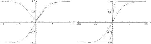
Fig. 1.
The left panel shows profiles of HiL (solid line), HiR (long-dashed line), and σi (dashed line) with finite gauge coupling (gi = 0.5). The right panel shows a plot of σi: dashed curve for finite (gi = 0.5) gauge coupling and solid curve for strong gauge coupling (|$g_i=\infty $|). The other parameters are mi = vi = 1.
One can take, if one wishes, the strong gauge coupling limit of the Lagrangian
|$\mathcal {L}_i$|. As is well known, the
U(1) gauge theory with two flavors of Higgs scalars in the strong gauge coupling limit becomes a nonlinear sigma model whose target space is
|$\mathbb {C}P^1$|:
The gauge fields and the neutral scalar field become infinitely massive and lose their kinetic terms. They are mere Lagrange multipliers in the limit, and are solved as
Plugging these into
|$\mathcal {L}_i$|, we get
with a projection operator
Let us introduce an inhomogeneous coordinate
ϕi of
|$\mathbb {C}P^1$| by
Then the Lagrangian of the
|$\mathbb {C}P^1$| model in terms of
ϕi is
Let us reconsider the domain wall solutions in this limit. The Hamiltonian can be written as
The BPS equation and the boundary conditions are given by
corresponding to the boundary conditions in Eq. (
2.9). The BPS equation can be easily solved by
The tension of the domain wall is
This is the same as the one in the finite gauge coupling model.
In this way, the strong gauge coupling limit has a great advantage compared to the finite gauge coupling case. One can exactly solve the BPS equation and see the moduli parameter in the analytic solutions. Furthermore, there are no important differences between domain wall solutions in the finite coupling (Abelian–Higgs model) and the strong coupling (nonlinear sigma model). Both solutions have the same domain wall tension and the same number of moduli parameters. To see the difference explicitly, let us compare the configuration of the neutral scalar field
σi. In the strong gauge coupling limit, it can be written as
where we have used
In Fig.
1, we show the configurations of
σi in two cases, one in the small finite gauge coupling and one in the strong gauge coupling limit. As can be seen from the figure, there are no significant differences.
Let us next derive the low-energy effective theory on the domain wall. We integrate all the massive modes while keeping the massless modes. We use the so-called moduli approximation, where the dependence on (3 + 1)-dimensional spacetime coordinates comes into the effective Lagrangian only through the moduli fields:
The effective Lagrangian for the moduli field
Ci(
xμ) can be obtained by plugging this into the Lagrangian
|$\mathcal {L}_i$| and integrating it over
y. This can be done explicitly as follows.
With Eq. (
2.31), the effective Lagrangian is given by
where the energy of the soliton solution is neglected since it does not contribute to the moduli dynamics. Note that
|$2m_iv_i^2$| is precisely the domain wall tension. This is the free-field Lagrangian.
Although we have derived this effective Lagrangian in the strong gauge coupling limit, we can obtain the same Lagrangian in the finite gauge coupling constant. In other words, the effective Lagrangian cannot distinguish the infinite versus finite coupling cases, at least in the quadratic order of the derivative expansion.
2.2 Localization of the Abelian gauge fields
In the previous subsection, we have seen that the NG modes of the translation and U(1) global symmetry are the only massless modes in the Abelian–Higgs model. They are localized on the domain wall. There are no massless gauge fields on the domain wall and all the modes contained in the gauge field are massive. The mass of the lightest mode of the gauge field is of the order of the inverse of the width of the domain wall, since the bulk outside the domain wall is in the Higgs phase. The low-energy effective Lagrangian for the massless fields is obtained after integrating out the massive modes, including gauge fields.
In order to obtain the massless gauge field localized on the domain wall, we need a new gauge symmetry that is unbroken in the bulk. Recently, a new mechanism was proposed to localize gauge fields on domain walls [18].
A key ingredient is the so-called dielectric coupling constant [
14–17] for the new gauge symmetry. To illustrate the new localization mechanism, let us introduce a new
U(1) gauge field
aM that we wish to localize on the domain wall. Since this gauge symmetry should be unbroken in the bulk, we consider the case where all the Higgs fields are neutral under this newly introduced
U(1) gauge symmetry. The gauge field
aM is assumed to couple to the neutral scalar fields
σi only in the following particular combination:
where a real constant
λ has the unit mass dimension, in accordance with the (4 + 1)-dimensional spacetime, and the field strength is defined by
The field-dependent gauge coupling function is given by
which depends on the position
y through fields
σi. Thus the field-dependent gauge coupling function
e(
σ) plays the role of the dielectric coupling constant. Furthermore, the special choice in Eq. (
2.37) is chosen for the gauge interaction to become strongly coupled in the bulk (
σi → ±
mi as
|$y \to \pm \infty $|).
Let us again consider a double copy of domain walls as a background configuration in the Abelian–Higgs model in Eq. (
2.35). Since the Lagrangian has no term linear in
aM, the equations of motion for
aM are trivially solved by
aM = 0, and the rest of the equations of motion are explicitly the same as those in the previous subsection. Therefore the domain wall solution in the previous subsection together with
aM = 0 is still a solution of the equations of motion. Clearly, the low-energy effective Lagrangian on the domain wall is also unchanged:
except for the additional kinetic term (the last term) of the (3 + 1)-dimensional gauge field
wμ, which is the zero mode (
y-independent mode) of the (4 + 1)-dimensional field
wμ. The (3 + 1)-dimensional gauge coupling constant is given by
where we have used the asymptotic behavior
|$\psi _i \to \log 2\cosh 2m_i(y-y_i)$| as
|$|y| \to \infty $|. Note that this result is again independent of the gauge couplings
gi in the domain wall sector. In summary, the low-energy effective Lagrangian is
Now we separate the quantum fields (fluctuations) from the classical background moduli parameters by
Then the effective Lagrangian up to the second order of the small quantum fluctuations is given by
We note that the massless gauge field
aμ has a positive finite gauge coupling squared
2 ,
|$1/(4\lambda (y_2^0-y_1^0))$|, provided
|$y_2^0-y_1^0>0$|.
Although we succeeded in localizing the massless
U(1) gauge field
aμ on the domain walls, the Lagrangian Eq. (
2.42) has no charged matter fields minimally coupled with the localized gauge field
aμ. To obtain matter fields interacting with the localized gauge field, one may be tempted to identify the Higgs fields
Hi = (
HiL,
HiR) as matter fields
3 with charges (1,−1). The minimal gauge interaction of Higgs fields with
aM is introduced through the modified covariant derivatives as
Since the moduli field
Ci is charged, the derivatives in the low-energy effective theory Eq. (
2.33) should be replaced by the covariant derivative
It is a straightforward task to derive the effective Lagrangian with the covariant derivative above along the same line of reasoning for the previous case:
This clearly shows that the new gauge field
aμ is not massless due to the Higgs mechanism, and should be integrated out together with the other massive fields. Namely, the low-energy effective Lagrangian does not include the massless gauge fields, since the
U(1) symmetry that we gauged is broken by the domain wall. A more explicit example at the strong gauge coupling limit is described in Appendix A. Thus the Abelian–Higgs model in this section provides an important lesson that we should not gauge a symmetry that is broken by the domain wall solution, since the corresponding gauge fields may be localized on the domain walls but they become massive and should be integrated out from the low-energy effective theory. In the next section, we will give a model with a non-Abelian global symmetry whose unbroken subgroup can be gauged to yield massless localized gauge fields on the domain wall.
3. The chiral model
In this section we study domain walls in the chiral model, which is a natural extension of the Abelian–Higgs model in the previous section. This chiral model leads to two important consequences: 1) massless non-Abelian gauge fields are localized on the domain wall and, moreover, 2) the scalar fields that are nontrivially interacting are also localized on the domain walls.
3.1 The domain walls in the chiral model
As a natural extension of the domain wall sector in the previous section, we consider the Yang–Mills–Higgs model with SU(N)c × U(1) gauge symmetry with S[U(N)L × U(N)R] = SU(N)L × SU(N)R × U(1)A flavor symmetry [19,26]. To localize the gauge field in a simple manner, we again introduce two sectors |$\mathcal {L}_1$| and |$\mathcal {L}_2$|, but only the former is extended to the Yang–Mills–Higgs system; the latter has the same form as (2.1). The second sector couples to the first sector through the coupling as described in (2.35); after gauging the flavor symmetry it plays a role in the localization of gauge fields, combined with the first sector. The matter contents are summarized in Table 1. Since the presence of two factors of SU(N) global symmetry resembles the chiral symmetry of QCD, we call this Yang-Mills-Higgs system the chiral model.
Table 1.Quantum numbers of the domain wall sectors in the chiral model.
|
. | SU(N)c
. | U(1)1
. | U(1)2
. | SU(N)L
. | SU(N)R
. | U(1)1A
. | U(1)2A
. | mass
. |
|---|
| H1L | |$\square $| | 1 | 0 | |$\square $| | 1 | 1 | 0 | m11N |
| H1R | |$\square $| | 1 | 0 | 1 | |$\square $| | −1 | 0 | −m11N |
| Σ1 | adj ⊕ 1 | 0 | 0 | 1 | 1 | 0 | 0 | 0 |
| H2L | 1 | 0 | 1 | 1 | 1 | 0 | 1 | m2 |
| H2R | 1 | 0 | 1 | 1 | 1 | 0 | −1 | −m2 |
| Σ2 | 1 | 0 | 0 | 1 | 1 | 0 | 0 | 0 |
The Lagrangian is then given by
with
|$H_1 = \left (H_{1L},\ H_{2L}\right)$|.
|$\mathcal {L}_2$| has the same form as (
2.1) with
i = 2. Gauge fields of
U(
N)
c = (
SU(
N)
c ×
U(1)
1)/
ZN are denoted as
W1M, and adjoint scalar as Σ
1. The covariant derivative and the field strength are denoted as
|$\mathcal {D}_M\Sigma _1 = \partial _M \Sigma _1 + i \left [W_{1M}, \Sigma _1\right ]$|,
|$\mathcal {D}_M H_1 = \partial _M H_1 + i W_{1M} H_1$|, and
|$F_{1MN} = \partial _M W_{1N} - \partial _N W_{1M} + i \left [W_{1M},W_{1N}\right ]$|. The mass matrix is given by
|$M_1 = {\mathrm {diag}}\left (m_1 \textbf {1}_N, -m_1\textbf {1}_N\right)$|. Let us note that the chiral model reduces to the Abelian–Higgs model in the limit of
N → 1, by deleting all the
SU(
N) groups.
The second sector is just necessary to realize the field-dependent gauge coupling function similar to (
2.35), as we will discuss in the next subsection. In the rest of this subsection, we focus only on the first sector (
i = 1) and suppress the index
i = 1. The symmetry transformations act on the fields as
with
Uc ∈
U(
N)
c,
UL ∈
SU(
N)
L,
U(
N)
R ∈
SU(
N)
R and
eiα ∈
U(1)
A.
There exist
N + 1 vacua in which the fields develop the following VEV:
with
r = 0,1,2,⋯,
N. We refer to these vacua with the label
r. In the
rth vacuum, both the local gauge symmetry
U(
N)
c and the global symmetry are broken, but the diagonal global symmetries are unbroken (color–flavor-locking):
As in the Abelian–Higgs model, the BPS equations for the domain walls can be obtained through the Bogomol'nyi completion of the energy density with the assumption that all the fields depend on only the fifth coordinate
y and
Wμ = 0:
This bound is saturated when the following BPS equations are satisfied:
The tension of the domain wall is given by
Let us concentrate on the domain wall that connects the 0th vacuum at
|$y\to \infty $| and the
Nth vacuum at
|$y \to -\infty $|. Its tension can be read as
from Eq. (
3.12). Since there are
N + 1 possible vacua, the maximal number of walls is
N at various positions. The simplest domain wall solution corresponding to the coincident walls is given by making an ansatz that
HL,
HR, Σ, and
Wy are all proportional to the unit matrix. Then the BPS equations (
3.10) and (
3.11) can be identified with the BPS equations in Eq. (
2.8) in the Abelian–Higgs model. Thus the domain wall solution can be solved as
where
ψ is the solution of the master equation (
2.12) in the Abelian–Higgs model. Equation (
3.8) shows that the unbroken global symmetry for the
Nth vacuum (
HL = 0,
HR =
v1N and Σ = −
m1N) at the left infinity
|$y \to -\infty $| is
SU(
N)
L ×
SU(
N)
R + c ×
U(1)
A + c, whereas that for the 0th vacuum (
HL =
v1N,
HR = 0, and Σ =
m1N) at the right infinity
|$y\to \infty $| is
SU(
N)
L + c ×
SU(
N)
R ×
U(1)
A + c.
The domain wall solution further breaks these unbroken symmetries because it interpolates the two vacua. The breaking pattern by the domain wall is
4 This spontaneous breaking of the global symmetry gives NG modes on the domain wall as massless degrees of freedom valued on the coset, similarly to chiral symmetry breaking in QCD:
Since our model can be embedded into a supersymmetric field theory, these NG modes (
U(
N) chiral fields) appear as complex scalar fields accompanied with additional
N2 pseudo-NG modes
5 .
3.2 Localization of the matter fields
In the remainder of this subsection, we will give the low-energy effective Lagrangian on the domain walls where the massless moduli fields (the matter fields) are localized. The best way to parametrize these massless moduli fields is to use the moduli matrix formalism [
19–22]
where
S ∈
GL(
N,
C) and Ω =
SS† is the solution of the following master equation
where
We have used the
V -transformation to identify the moduli
eϕ, which is a complex
N by
N matrix. It can be parametrized by an
N ×
N Hermitian matrix
|$\hat {x}$| and a unitary matrix
U as [
19]
where
U is nothing but the
U(
N) chiral fields associated with the spontaneous symmetry breaking Eq. (
3.18) and
|$\hat {x}$| is the pseudo-NG modes whose existence we promised above.
In the strong gauge coupling limit
|$g \to \infty $|, the solution of the master equation is simply Ω = Ω
0. After fixing the
U(
N)
c gauge, we obtain
Let us denote, for brevity,
the Higgs fields are then given as
From this solution, one can easily recognize that eigenvalues of
|$\hat {x}$| correspond to the positions of the
N domain walls in the
y direction. Now we promote the moduli parameters
|$\hat {x}$| and
U to fields on the domain wall world volume, namely functions of world volume coordinates
xμ. We plug the domain wall solutions
|$H_{L,R}(y; \hat {x}(x^\mu),U(x^\mu))$| into the original Lagrangian
|$\mathcal {L}$| in Eq. (
3.2) at
|$g \to \infty $| and pick up the quadratic terms in the derivatives. Thus the low-energy effective Lagrangian is given by [
27]
where
Here we have eliminated the massive gauge field Wμ by using the equation of motion. Using the solutions for HL and HR we have found a closed formula for the effective Lagrangian up to the second order of derivatives but with full nonlinear interactions involving moduli fields |$\hat {x}$| and U. The detailed derivation is given in Appendix B.
Here we exhibit the results only in the leading orders of
U − 1 and
|$\hat {x}$|:
When
N = 1 and with the redefinitions
U =
e2iα1 and
|$\hat {x} = 2m y_1$|, this coincides with the effective Lagrangian
|$\mathcal {L}_{i=1,{\mathrm {eff}}}$| in Eq. (
2.34) of the Abelian–Higgs model, which we obtained in the previous section.
3.3 Localization of the gauge fields
Let us next introduce the gauge fields that are to be massless and localized on the domain walls. As we learned in Sect. 2, the associated gauge symmetry should not be broken by the domain walls. Therefore, the symmetry that we can gauge is the unbroken symmetry SU(N)L + R + c itself or its subgroup.
Let us gauge
SU(
N)
L + R≡
SU(
N)
V and let
|$A_{\mu }^a$| be the
SU(
N)
L + R gauge field. The Higgs fields are in the bi-fundamental representation of
U(
N)
c and
SU(
N)
L + R. The covariant derivatives of the Higgs fields are modified by
The quantum numbers are summarized in Table
2.
Table 2.Quantum numbers of the domain wall sectors in the gauged chiral model.
|
. | SU(N)c
. | U(1)1
. | U(1)2
. | SU(N)V
. | U(1)1A
. | U(1)2A
. | mass
. |
|---|
| H1L | |$\square $| | 1 | 0 | |$\square $| | 1 | 0 | m11N |
| H1R | |$\square $| | 1 | 0 | |$\square $| | −1 | 0 | −m11N |
| Σ1 | adj⊕1 | 0 | 0 | 1 | 0 | 0 | 0 |
| H2L | 1 | 0 | 1 | 1 | 0 | 1 | m2 |
| H2R | 1 | 0 | 1 | 1 | 0 | −1 | −m2 |
| Σ2 | 1 | 0 | 0 | 1 | 0 | 0 | 0 |
We now introduce a field-dependent gauge coupling function
g2(Σ) for
AM, which is inspired by the supersymmetric model in Ref. [
18]).
The Lagrangian is given by
The
|$\tilde {\mathcal {L}}_1$| in Eq. (
3.34) is given by Eq. (
3.2) where the covariant derivatives are replaced with those in Eqs. (
3.31) and (
3.32).
We first wish to find the domain wall solutions in this extended model. As before, we make an ansatz that all the fields depend on only
y and
Wμ =
Aμ = 0. Let us first look at the equation of motion of the new gauge field
AM. It is of the form
where
JM stands for the current of
AM. Note that the current
JM is zero, by definition, if we plug the domain wall solutions into the chiral model before gauging
SU(
N)
L + R. This is because the domain wall configurations do not break
SU(
N)
L + R. Therefore,
AM = 0 is a solution of Eq. (
3.35).
Then, we are left with the equation of motion with AM = 0, which is identical to those in the ungauged chiral model in the previous subsections. Therefore the gauged chiral model admits the same domain wall solutions as those (Eqs. (3.26) and (3.27)) in the ungauged chiral model.
The next step is to derive the low-energy effective theory on the domain wall world volume in the moduli approximation, as in the previous subsections. Again, we promote the moduli parameters as fields on the domain wall world volume and pick up the terms up to the quadratic order of the derivative ∂μ. Similarly to Sect. 3.2, we utilize the strong gauge coupling limit |$g_i \to \infty $|, to simplify the computation without changing the final result. Let us emphasize that we keep the field-dependent gauge coupling function e(Σ) finite. The spectrum of massless NG modes is unchanged by switching on the SU(N)L + R gauge interactions6 .
We just repeat a similar computation to those in Sect.
3.2. Again, we shall focus on the first sector
|$\mathcal {L}_1$| and suppress the index
i = 1 of fields. Since the color gauge fields
Wμ become auxiliary fields and are eliminated through their equations of motion, it is convenient to define the covariant derivative only for the flavor (
SU(
N)
L + R) gauge interactions as
Then we obtain the effective Lagrangian of the first sector as
with
Eliminating
Wμ, we obtain the following expression for the integrand of the effective Lagrangian after some simplification:
where we define fields
Hab with the label
ab of the adjoint representation of the flavor gauge group
SU(
N)
L + R + c and the covariant derivative as
In Appendix B, we will describe fully the procedure to derive the effective Lagrangian by substituting (
3.26) and (
3.27) and rewriting
|$\hat {x}$| and
U in terms of moduli fields. Here we merely state the result:
where
is a Lie derivative with respect to
A. The covariant derivative
|$\mathcal {D}_\mu $| is defined by
The above result suggests that the chiral fields
U(
xμ) and Hermitian fields
|$\hat {x}(x^{\mu })$| are in the adjoint representation of
SU(
N)
L + R. Let us now examine the transformation property of
U and
|$\hat {x}$| under the
SU(
N)
L + R flavor gauge transformation on the domain wall background in order to demonstrate that they are in the adjoint representation. The domain wall solution only preserves the diagonal subgroup
SU(
N)
L + R + c. Equations (
3.4) and (
3.5) shows that the fields transform under the
SU(
N)
L + R + c transformations
|$\mathcal {U}$| as
Equations (
3.19) and (
3.20) show that
The complex moduli
eϕ is decomposed into a Hermitian part
|$e^{\hat {x}}$| and a unitary part
U in Eq. (
3.23). Since we can express
|$e^{2\hat {x}}=e^{\phi } e^{{\phi }^{\dagger }}$| and
|$U=e^{-\phi }e^{\hat {x}}$|, we find that they transform as adjoint representations
By expanding (
3.41), we here illustrate nonlinear interactions of
|$\hat {x}$| up to fourth orders in the fluctuations
|$\hat {x}$| and
U−
1:
Similarly to Eq. (
2.39), we can define the (3 + 1)-dimensional non-Abelian gauge coupling
e4 by integrating (
3.33) and find
where
yi is the wall position for the
ith domain wall sector. Summarizing, we obtain the following effective Lagrangian:
where
|$\mathcal {L}_{2, {\rm eff}}$| is given in (
2.34). This is the main result of this paper. We have succeeded in constructing the low-energy effective theory in which the matter fields (the chiral fields) and the non-Abelian gauge fields are localized with the nontrivial interaction. We show the profile of “wave functions” of the localized massless gauge field and massless matter fields as functions of the coordinate
y of the extra dimension in Fig.
2.
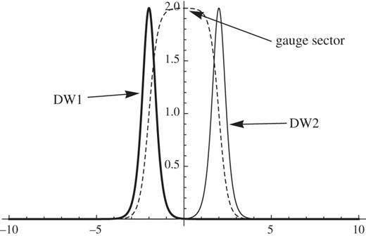
Fig. 2.
The wave functions of the zero modes. DW1 and DW2 stand for the wave functions of the massless matter fields of the i = 1 domain wall and the i = 2 domain wall, respectively, for the strong gauge coupling limit |$g_i=\infty $| and mi = 1. The gauge fields are localized between the domain walls.
As is seen from Eq. (3.47), the flavor gauge symmetry SU(N)L + R + c is further (partly) broken and the corresponding gauge field Aμ becomes massive when the fluctuation |$\phi = e^{\hat {x}} U$| develops nonzero vacuum expectation values. In particular, |$\hat {x}$| is interesting because its non-vanishing (diagonal) values for the fluctuation have physical meaning as the separation between walls away from the coincident case. For instance, if all the walls are separated, SU(N)L + R + c is spontaneously broken to the maximal U(1) subgroup U(1)N−1. However, if r walls are still coincident and all other walls are separated, we have an unbroken gauge symmetry SU(r) × U(1)N−r + 1. Then, part of the pseudo-NG modes |$\hat {x}$| become NG modes associated with further symmetry breaking SU(N)L + R + c→SU(r) × U(1)N−r + 1, so that the total number of zero modes is preserved[19]7 . These new NG modes, called the non-Abelian cloud, spread between the separated domain walls[19]. The flavor gauge fields eat the non-Abelian cloud and attain masses that are proportional to the separation of the domain walls. This is the Higgs mechanism in our model. This geometrical understanding of the Higgs mechanism is quite similar to D-brane systems in superstring theory. So our domain wall system provides a genuine prototype of field theoretical D3-branes.
4. Embedding into supersymmetric theory
A crucial point to localize the gauge field around the domain wall is the coupling between the scalar and gauge kinetic terms. Such a coupling is naturally realized in (4 + 1)-dimensional supersymmetric gauge theory [18]. This theory generally consists of a hypermultiplet part and a vector multiplet part. The latter is specified by the so-called prepotential. In (4 + 1)-dimensional theory the prepotential generally allows up to cubic terms in vector multiplets[25], which serve as interactions between vector mutiplets such as (3.33).
4.1 Supersymmetric model
In embedding the model into supersymmetric gauge theories in (4 + 1) dimensions, we will give the non-Abelian global flavor symmetry
SU(
Ni)
V for each copy (
i = 1,2) of the domain wall sector, instead of only one copy as in (
3.34) in the previous section. This contains the model (
3.34) as a limiting case of
N2→1, and may offer a more general situation phenomenologically. To formulate supersymmetric gauge theories, we need to introduce
Yi as auxiliary fields of the
U(
Ni)
c vector multiplet, and Φ
i and
|$\mathcal {Y}_i$| as adjoint scalar fields and auxiliary fields of the
SU(
Ni)
V vector multiplet. As bosonic fields of theories with eight supercharges, we also need to double the scalar fields
Hi, by introducing another set
|$\tilde {H}^{\dagger }_i = (\tilde {H}_{iL}^{\dagger }, \tilde {H}_{iR}^{\dagger })$| with masses (
mi1Ni,−
mi1Ni). They are in the same representations as
Hi under
U(
Ni)
c and
U(1)
iA. Explicit charge assignments for the hypermultiplet matter fields and adjoint scalar fields are summarized in Table
3. The resultant supersymmetric Lagrangian is written as
where
where
α,
β⋯ denote all gauge groups and their generators collectively. We label them with the ordering
where 0
i denotes the
U(1)
i parts of the
U(
Ni)
c gauge group, while
|$I_i=1, \ldots , N_i^2-1$| are color indices of
SU(
Ni)
c and
|$A_i=1, \ldots , N_i^2-1$| denotes the flavor indices of the
SU(
Ni)
V gauge group. The scalar fields Σ
α and auxiliary fields
Yα are explicitly given by
and similarly the field strength
|$F_{MN}^\alpha $| and gauge field
|$W_{M}^\alpha $| are given by
We adopt the convention of
U(
Ni)
c and
SU(
Ni)
V matrices such as
Covariant derivatives for
HiL and
HiR are given as (
3.31) and (
3.32) with identical definitions for
|$\tilde {H}_{iL}^{\dagger }$||$\tilde {H}_{iR}^{\dagger }$|. Covariant derivatives of Σ
Ii,Φ
Ai are defined as the adjoint representation. We will not display the Chern–Simons term
|$\mathcal {L}_{i\mathrm {CS}}$| and the fermionic term
|$\mathcal {L}_{i\mathrm {fermion}}$|, since we do not need them for our analysis.
Table 3.Quantum numbers of hypermultiplets |$(H_i,\tilde {H}_i)$|, Σi, and Φi.
|
. | U(Ni)c
. | U(1)iA
. | SU(Ni)V
. | mass
. |
|---|
| HiL | |$\Box $| | 1 | |$\Box $| | mi1Ni |
| HiR | |$\Box $| | 1 | |$\Box $| | −mi1Ni |
| |$\tilde {H}_{iL}$| | |$\bar {\Box }$| | −1 | |$\bar {\Box }$| | mi1Ni |
| |$\tilde {H}_{iL}$| | |$\bar {\Box }$| | −1 | |$\bar {\Box }$| | −mi1Ni |
| Σi | adj | 0 | 1 | 0 |
| Φi | 1 | 0 | adj | 0 |
Functions
aαβ(Σ) are gauge coupling functions, which are given as a second derivative of the prepotential
From the above prepotential, we see the coupling constants of
U(1)
i and
SU(
Ni)
c are given by
|$\hat {g}_i$| and
gi, respectively
8 . We denote the coupling function of
SU(
Ni)
V corresponding to Σ
α = Φ
Ai and Σ
β = Φ
Bi as
ei(Σ),
but will suppress the argument Σ to write
ei in the following.
The constants
cα are coefficients of the Fayet–Iliopoulos (FI) terms, allowed to be nonzero only for the
U(1) part of the gauge groups
9 We have assumed both the FI parameters
c01 and
c02 to be positive in the same direction in
SU(2)
R, which is chosen to be along the third component. In this setup, the
|$\tilde {H}$| fields will vanish in the classical solution. Moreover, they do not contribute to the desired order of the effective Lagrangian. Similarly, we have neglected the auxiliary fields
Y other than the third component in
SU(2)
R, which we have denoted as
Yα. Hence we can call the potential after eliminating the auxiliary fields
Y the D-term potential.
The F-term potential
ViF can be worked out from the following superpotential:
where we restored the tilde fields
|$\tilde {H}$| to facilitate the writing of the superpotential. After eliminating the auxiliary fields
F, and with the use of
we have (
4.3).
Finally, let us work out explicit forms of the D-term potential
VD. Collecting terms containing the auxiliary fields
Y , we obtain
where
are Hermitian matrices, with the decomposition
We observe that, in the potential (
4.17),
YIi do not couple to the rest of the auxiliary fields and can be easily eliminated. Having done this, we collect the
U(1)
i and
SU(
Ni)
V terms into a matrix form labeled by
α,
β = 0
1,0
2,
A1,
A2:
Eliminating the remaining auxiliary fields, we obtain:
Matrix
G = (
Gαβ) is explicitly given by
with the inverse
where we have abbreviated:
4.2 Positivity of potential
The F-term potential (
4.3) is manifestly positive. The D-term potential (
4.21) is positive definite under certain conditions. To find the conditions, we shall decompose (
4.21) to:
It is clear that the
V1D is positive definite by itself. Therefore we can only focus on
V2D, which is positive if and only if
G is positive definite.
It is easy to recognize that the positivity of G is manifest once the adjoint scalars vanish, Φi = 0. Nevertheless, it is instructive and assuring if we consider the potential as well as the BPS equations, keeping the adjoint scalars Φi nonzero.
To ascertain the positivity of
G we need to compute its eigenvalues. This is most easily done by looking at its determinant (we leave the derivation of this result to Appendix C):
Requiring det
G > 0, we have
In Appendix C we show that this condition is both necessary and sufficient to ensure the positivity of matrix
G in Eq. (
4.24).
4.3 BPS equations
Let us denote the codimension of the domain wall as y. Since we assume Lorentz invariance for the other dimensions, we obtain a vanishing gauge field for components other than y.
The energy density
|$\mathcal {H}$| for domain walls is given by
where the color–flavor indices
α,
β span all values as in Eq. (
4.4) and we have incorporated the color sector
α =
I1,
I2 into the definition of matrix
G for brevity. Accordingly, we have incorporated the definition (
r−
c)
Ii =
rIi. Since there is no mixing of the color sector with the rest, the inverse is calculated trivially and the non-color part remains the same as in (
4.1).
Now we observe that the mixing due to the cubic prepotential occurs only in the kinetic term and potential of the vector multiplets. Moreover, they appear as G and G−1 respectively. Therefore the cross term coming out of the Bogomol'nyi completion has no dependence on the metric G. This fact implies that the cancellation of cross terms to give topological charge goes through unaffected by the mixing of the vector multiplets.
More explicitly, we obtain the Bogomol'nyi completion as
The last term gives the usual Bogomol'nyi bound and becomes the topological charge. The line before that is the total derivative, which gives a vanishing contribution for an infinite line
|$-\infty < y < \infty $|.
The BPS equations for
H and
|$\tilde {H}$| of hypermultiplets are
The BPS equations for vector multiplets are
More explicitly,
We can easily solve the BPS equation for hypermultiplets by using the moduli matrix approach. We define
Sic,
SiF, and
ψi as
Then the hypermultiplet BPS equations (
4.37)–(
4.40) are solved by the constant moduli matrices
|$H_{iL}^{0}$| and
|$H_{iR}^{0}$|:
where
|$S_{ic}, S_{iF} \in SL(N_i,\mathbb {C})$|. The hypermultiplet fields
|$\tilde {H}_{iL}$| and
|$\tilde {H}_{iR}$| do not contribute to the domain wall solution and they are therefore vanishing. We write down (
4.42)–(
4.44) in terms of the gauge invariant fields:
The adjoint scalar fields of the vector multiplets are given by
Also, we have
The BPS equations for vector multiplets (
4.42)–(
4.44) can now be rewritten as the following master equations:
Here we have used the notation
We make a comment about the possibility of additional moduli. At present we cannot say definitely if there are additional moduli other than the moduli matrices
H0, since we cannot solve these master equations. We have several clues at hand. The BPS equations for domain walls and other solitons in gauge theories with scalar fields in the fundamental representations are in the Higgs phase where all the gauge symmetries are broken in the vacuum. In this situation, we have learned that all the moduli are contained in the moduli matrix. On the other hand, instantons are solitons in pure Yang–Mills theory without scalar fields, where the gauge symmetry is unbroken in the vacuum. In this case, moduli reside in the BPS equation for gauge fields. In our present case, unbroken gauge symmetry
SU(
Ni)
c + V remains. This feature is indicative of additional moduli coming from the vector multiplet.
Irrespective of the possible additional moduli, we can demonstrate that the BPS equations admit the coincident wall solution. Since the hypermultiplet parts are already solved as in (
4.47)–(
4.48), our main task is to solve the master equations (
4.54)–(
4.56) associated with the vector multiplet. In order to solve them explicitly, we take the strong gauge coupling limit
|$\hat {g}_i, g_i\rightarrow \infty $|, where the master equations give just the algebraic constraints for Ω
ic, Ω
iF, and
ηi. In principle, they can be solved algebraically. Furthermore, Eq. (
4.34) with the limit
|$g_i\rightarrow \infty $| tells us that positivity is maintained only if Φ
i vanishes. In the following we will, therefore, consider a special point in the solution space where
which implies from Eq. (
4.51) that Ω
iF are constant matrices. Then the differential equations (
4.55)–(
4.56) reduce to a set of algebraic equations:
Notice that for both sectors
i = 1,2 these equations are the same and do not couple to each other. We can, therefore, focus our discussion only on one sector, since all results are equivalent in both of them. So in the remaining discussion we will drop the index
i from all fields.
Now we consider moduli matrix for the coincident walls corresponding to the most symmetric point of the moduli space.
Equations (
4.59) and (
4.60) show that these two constant matrices commute and only the product Ω
cΩ
F = Ω
FΩ
c can be determined
10 :
Since we have chosen the matrices
Sc,
SF in
|$SL(N,\mathbb {C})$|, we find that det(Ω
cΩ
F) = 1 and we can separate the
U(1) part.
The
U(1) part gives the usual domain wall solution. Without affecting the physical quantities, we can choose Ω
c = 1,
Sc = 1, and finally we obtain the coincident wall solution for (
4.61) with (
4.58) and with the wall position moduli
y0 (modifying (
4.61) to
|$(H_L^0, H_R^0) =(e^{-my_0}, e^{my_0}))$|:
Note that in this solution we restore a moduli parameter
y0 corresponding to the position of the coincident wall. A similar construction of the domain wall solution works for the second sector (
i = 2), besides the first sector (
i = 1) given above.
Let us note that the field-dependent gauge coupling function, like (3.33), is automatically obtained as a bosonic part of the Lagrangian specified by the cubic prepotential in Eq. (4.11). Restoring the index i = 1,2 for both of the domain wall sectors, and by using (4.65) with (4.50), we finally conclude that an appropriate profile for the field-dependent gauge coupling function Σ01/m1−Σ02/m2, like (3.33), is achieved. When we make (part of) the global flavor symmetry a local gauge symmetry, we can have several options. Since the first flavor group SU(N1) is generally different from the second flavor group SU(N2), we can naturally introduce two different gauge fields for i = 1 and 2. This option leads to two decoupled sectors in the low-energy effective Lagrangian, which can only be coupled by higher derivative terms induced by massive modes. Another interesting option is to introduce a gauge field only for the diagonal subgroup of isomorphic subgroups of two different flavor groups, such as |$SU(\tilde {N}) \in SU(N_1)$|, |$SU(\tilde {N})\in SU(N_2)$| with |$\tilde {N} \le N_1, N_2$|. This option is interesting in the sense that the massless gauge field exchange will communicate between two domain wall sectors. We hope to come back to these issues in the near future.
Let us make a few comments. First, we have shown that the chiral model analyzed in Sect. 3 can be extended to a supersymmetric gauge theory with eight supercharges and that the field-dependent gauge coupling function, which is a clue for localization, is naturally explained by taking the cubic prepotential. Second, there may be more moduli not contained in |$(H_{L}^0,H_{R}^0)$|, which require further studies. Third, here we have presented a solution at a special point Φ = 0. It would be interesting to consider the case for Φ≠0, but, in this case, we need to take a finite gauge coupling limit, which we will investigate in future work.
5. Conclusions and discussion
In this paper we have successfully localized both massless non-Abelian gauge fields and massless matter fields in a nontrivial representation of the gauge group. We first considered a (4 + 1)-dimensional U(N) gauge theory with additional SU(N)L × SU(N)R × U(1)A flavor symmetry. We introduced the flavor gauge field for the diagonal flavor group SU(N)L + R, which is unbroken in the coincident wall background. The flavor gauge fields are localized on the wall by introducing the scalar-field-dependent gauge coupling function. Then we studied the low-energy effective Lagrangian and showed that massless localized matter fields interact minimally with localized SU(N)L + R gauge field as adjoint representations. Moreover, the full nonlinear interaction between moduli containing up to second derivatives was worked out. The field-dependent gauge coupling function is naturally realized in supersymmetric gauge theories using the so-called prepotential. For this reason, we also explored the bosonic part of the |$\mathcal {N}=1$| supersymmetric extension of our model.
The main result of this paper is the effective Lagrangian (3.49). The moduli field U appearing in the effective theory is a chiral N × N matrix field like a pion, since it is an NG boson of spontaneously broken chiral symmetry. Other moduli in (3.49), denoted by the N × N Hermitian matrix |$\hat {x}$|, have the physical meaning of the positions of N domain walls as their diagonal elements. We argued that the fluctuations of moduli field |$\hat {x}$| can develop VEV corresponding to splitting of walls, and the Higgs mechanism will occur as a result. Namely, the flavor gauge fields attain masses by eating the non-Abelian cloud. Therefore, in this model, the Higgs mechanism has a geometrical origin like low-energy effective theories on D-branes in superstring theory.
Amongst the possible future investigations, we would like to study the non-coincident solution to further clarify this geometrical Higgs mechanism. We have noticed that our effective moduli fields resemble the pion in QCD. Similar attempts have been quite successful using D-branes [28]. We believe that our methods can provide more insight into various aspects of low-energy hadron physics. We plan to explore this direction more fully in subsequent studies.
In the discussion of a supersymmetric extension of our model in Sect. 4, we employed a general setup where both sectors possessed their own domain wall solution, preserving the same half of the supercharges. But another alternative approach is also possible. We can consider a model in which different halves of supercharges are preserved at each sector (BPS and anti-BPS walls), and the SUSY is completely broken in the system as a whole. It has been proposed that the coexistence of BPS and anti-BPS walls gives supersymmetry breaking in a controlled manner [29,30]. In our present case, the BPS and anti-BPS sectors interact only weakly. If we choose the flavor gauge field for each sector separately, we have only higher derivative interactions induced by massive modes. If we choose the diagonal subgroup(s) of each sector to be a flavor gauge group, we have a more interesting possibility of the massless gauge field acting as a messenger between the two sectors. We plan to address this issue elsewhere.
In order to construct a realistic brane-world scenario with the SM fields on the domain wall, we need the localization of fields in the fundamental representation of the gauge group. This is still an open problem and one of the priorities of our future investigations. In particular, the SM contains chiral fermions. The localization of chiral fermions is a particularly challenging problem. The anomaly associated with the chiral fermion is also an interesting issue to be addressed. We would also like to clarify these problems in subsequent studies.
Two more issues remain to be addressed. First is the question of the sign of the gauge kinetic term. In our present model, the positivity of the gauge coupling function is assured only when the positions of walls are properly ordered [see Eq. (3.48)], namely only in a region of the moduli space. More economical models, such as those given in Ref. [18], may not have such moduli and, therefore, the effective gauge coupling may always be positive. And lastly, as discussed in Sect. 4, we have not succeeded in exhausting all moduli in the supersymmetric extension of our model. We would also like to investigate these aspects in the future.
Acknowledgements
This work is supported in part by the Japan Society for the Promotion of Science (JSPS) and the Academy of Sciences of the Czech Republic (ASCR) under the Japan–Czech Republic Research Cooperative Program, and by a Grant-in-Aid for Scientific Research from the Ministry of Education, Culture, Sports, Science and Technology, Japan No.21540279 (N.S.), No.21244036 (N.S.), and No.23740226 (M.E.). The work of M.A. and F.B. is supported in part by the Research Program MSM6840770029 and by the project of International Cooperation ATLAS–CERN of the Ministry of Education, Youth and Sports of the Czech Republic.
Appendix A
Domain walls in the gauged massive |$\mathbb {C}{\rm \textbf {P}}^{\textbf {1}}$| sigma model
Here we consider the domain wall solutions in the gauged massive
|$\mathbb {C}P^1$| sigma model. The model is obtained as the strong gauge coupling limit of a model similar to that we have studied in Sect.
2.2. Namely, we start with the Lagrangian that has
U(1) ×
U(1) gauge symmetry with two flavors:
where
H = (
HL,
HR). The covariant derivative is given by
The mass matrix is chosen as
M = diag(
m,−
m) as before.
We next take the strong gauge coupling limit
|$g\to \infty $| of only one of the gauge couplings that results in the nonlinear sigma model coupled to the other gauge field with the finite gauge coupling
e. In the limit, the gauge field
wM and the neutral scalar field
σ become Lagrange multipliers. After solving their equations of motion, we have
where we have introduced the covariant derivative
Plugging these into the original Lagrangian at
|$g\to \infty $|, we get the gauged massive
|$\mathbb {C}P^1$| sigma model
with the projection operator
As before, let us rewrite this Lagrangian with respect to the inhomogeneous coordinate
Then the charge matrix should be chosen as
which leads to a natural expression that the complex scalar field
ϕ has a
U(1) charge 1 for the gauge field
aM:
Plugging these into Eq. (
A.6), we finally get the Lagrangian
Let us next consider a domain wall solution in this model. We assume that all the fields depend on only the extra-dimensional coordinate
y. Then the four-dimensional components of the Maxwell equation
can be immediately solved by
The fifth component is
Now the Hamiltonian reduces to the following form:
Thus the reduced Hamiltonian is minimized when the following first-order equation is satisfied:
Since the mass parameter
m is real, Eq. (
A.15) is also satisfied. Let us take the gauge where
Then we have the explicit domain wall solution
This is identical to the domain wall solution given in Eq. (
2.28) in the ungauged massive
|$\mathbb {C}P^1$| sigma model.
The final step is to obtain a low-energy effective theory on the domain wall. The effective Lagrangian is given by
where we have promoted the moduli parameter
y0,
α to the fields
y0(
xμ),
α(
xμ) on the wall, and we have introduced the covariant derivative
where
α is a function of the (3 + 1)-dimensional coordinate
xμ. Assuming
aμ to be
y-independent (zero mode), we finally obtain
Thus we find that the gauge field
aμ(
x) absorbs the scalar field
α(
x) to become massive via the Higgs mechanism. Since the
U(1) gauge field
aμ is massive in the effective Lagrangian, we have to integrate it out according to the spirit of the low-energy effective theory.
Appendix B
Effective Lagrangian on the domain wall
In this appendix we derive our main result (3.41) of the effective Lagrangian for the gauged chiral model introduced in Sect. 3.
B.1. Compact form of the gauged nonlinear model
Starting from the Lagrangian using the Einstein summation convention for
a = {
L,
R}:
with the constraint
we first eliminate the gauge fields
Wμ to obtain a simple expression for the gauged nonlinear sigma model. Gauge fields
Wμ are given by equations of motion as
and
The effective Lagrangian (
B.1) should also contain a kinetic term for the gauge field
Aμ, but we will not explicitly write it here, for brevity. Equation (
B.1) can be further simplified by using the following identities:
where
After some algebra, we find:
Plugging the above expression back into (
B.1), we arrive at:
B.2. Effective Lagrangian
Now we are ready to compute the effective Lagrangian. Using a solution (with
|$\hat {y} = my\textbf {1}_N-\hat {x}$|),
Our new fields
Hab are given as:
It can be checked that (
B.8) is given as:
In the following, we would like to carry out the integration over the extra-dimensional coordinate
y. This can be done in two steps. First, we must factorize all quantities depending on
y (or on
|$\hat {y}$|) to one term inside the trace, effectively reducing our problem to fit the following form:
where
M is some matrix, independent of some function of
y and
f. In the second step we diagonalize
|$\hat {x}$|:
and use the fact that
|$f(P^{-1}\hat {y} P)=P^{-1}f(\hat {y})P$|. This transformation leads to
For every term in the sum we can perform the substitution
|$\tilde y = my-\lambda _i$|. The key observation is that in each term the integration will be the same and independent of a particular value of
λi. Thus we arrive at an identity
It appears as if we just made a substitution
|$\hat {y} = \tilde y\textbf {1}_N$|. This is possible, of course, only thanks to the diagonalization trick and properties of the trace. In the subsequent subsections, however, we will refer to this procedure as if it is just a ‘substitution’, for brevity. Let us decompose the effective Lagrangian (
B.13) into three pieces:
and see the outlined procedure for each term.
B.2.1. Kinetic term for U
First, let us concentrate only on terms containing double derivatives of
U, which we denote as
|$\mathcal {T}_{U}$|:
where we have used the fact that inside the commutator it is possible to freely interchange
since the difference is just a constant matrix. In this way we make
|$\mathcal {T}_{U}$| manifestly invariant under the exchange
|$\hat {y} \to -\hat {y}$|.
Since in the first factor of
|$\mathcal {T}_{U}$| all
|$\hat {y}$|-dependent quantities are on the right-hand side, we can, according to our previous discussion, make use of the identity (
B.15) and carry out the integration:
For the second term, however, we first use the identity:
where
|$\mathcal {L}_A(B) = \left [ A, B \right ]$| is a Lie derivative with respect to
A. Thus
Now all
|$\hat {y}$|-dependent factors are standing on the right and we can formally exchange
|$\hat {y} \to \tilde y$|. The summation can be carried out to obtain:
The formula for
|$\mathcal {T}_{U}$| now reads:
Since we started with
|$\mathcal {T}_{U}$| invariant under the transformation
|$\hat {y} \to -\hat {y}$|, we should take only the even part of the above formula (under exchange
|$\mathcal {L}_{\hat {x}} \to -\mathcal {L}_{\hat {x}}$|) as the final result:
Now we can carry out the integration using the primitive function
Therefore we obtain the result to all orders in
|$\hat {x}$| as:
Performing the Taylor-expansion of the function
we can easily read off the coefficients of terms beyond the leading one. For example, the first three terms read:
B.2.2. Mixed term
The mixed term between
|$\hat {x}$| and
U is given by
With use of the identity (
B.17) and
one can prove the following:
We can use this result to factorize all
|$\hat {y}$|-dependent quantities to the right and make the substitution
|$\hat {y} = \tilde y\textbf {1}_N$|:
Now we are free to perform summation and integration to obtain:
Performing the Taylor-expansion of the function
we can easily read off the coefficients of terms beyond the leading order in the series expansion:
B.2.3. Kinetic term for |$\hat {x}$|
The kinetic term for
|$\hat {x}$| is given by
We are going to need the identity
With the aid of this we arrive at
where we again employed the diagonalization trick and identity (
B.15). Let us carry out the summation and integration to obtain:
leading to the power series:
Putting all the pieces together as |$\mathcal {L}_{{\rm eff}} = \mathcal {T}_{\hat {x}} + \mathcal {T}_{U} +\mathcal {T}_{\rm mixed}$|, we obtain our final result (3.41).
Appendix C
Determinant of G
In order to calculate the determinant of matrix
G (
4.24) we will use the following recurrence formula, which relates the determinant of a symmetric matrix
|$\mathcal {M}$| of rank
N + 1 to the determinant of its
N ×
N submatrix
M:
After double application of formula (
C.2) we get
where
The inverse of
G1 is given as
where we have used (
4.26)–(
4.29).
Straightforward calculation leads us to
After multiplying both brackets we obtain the result (
4.33):
Next we would like to find the condition that ensures the positive definiteness of
G. In other words, we require that all eigenvalues of
G are non-negative. We can easily turn (
4.33) into a characteristic equation by replacing
|$\hat {g}_1^{-2},\hat {g}_2^{-2},e_1^{-2},e_2^{-2}$| with
|$\hat {g}_1^{-2}-\lambda ,\hat {g}_2^{-2}-\lambda $|,
|$e_1^{-2}-\lambda ,e_2^{-2}-\lambda $|. However, since
|$\tilde \Phi ^{2}$| consists of terms proportional to either
|$e_1^2$| or
|$e_2^2$| instead of
|$e_1^{-2}$| or
|$e_2^{-2}$|, we should first multiply the term in the square brackets by a factor
|$e_1^{-2}e_2^{-2}$|. Then, after the replacement and denoting
|$\Phi _i^2=\Phi ^{A_i}\Phi ^{A_i}, i=1,2$|, we obtain a characteristic equation of the fourth order:
multiplied by the factor
which clearly leads to positive eigenvalues. Expanding the brackets, we obtain explicit coefficients of the characteristic polynomial:
In order to see the non-negativeness of eigenvalues it is not necessary to solve the characteristic equation. Generally speaking, the characteristic equation of a real symmetric matrix can always be put into the form
where all roots
λ1,…
λN are real numbers. Multiplying all parentheses, we see that the coefficients
ck of the characteristic polynomial are given by the sum of all possible
k-tuples of
λ with alternating sign:
The positivity of all coefficients
ck turns out to be equivalent to the positivity of all eigenvalues
λk. To ensure the positivity of the eigenvalues, we now demand that all terms in (
C.11) inside brackets are positive. This gives us three conditions:
These can be put into the convenient form:
where
We are going to argue that the last condition
|$1-\tilde g^2\tilde \Phi ^2 \geq 0$| is the strongest one and, therefore, the only important one. This can be true if and only if the parameter
|$\tilde g^2$| is always greater then
|$\tilde g_{11}^2$|,
|$\tilde g_{12}^2$|,
|$\tilde g_{21}^2$|, and
|$\tilde g_{22}^2$| for all possible values of involved parameters. This is indeed so. Let us demonstrate this fact by showing, e.g.,
Multiplying both sides by
|$\hat {g}_1^2+\hat {g}_2^2+e_1^2+e_2^2$| and expanding our notation, we get
leading to
The last line is obviously always true. In the same way, one can show that
|$\tilde g^2 \geq \tilde g_{12}^2$|,
|$\tilde g^2 \geq \tilde g_{21}^2$|, and
|$\tilde g^2 \geq \tilde g_{22}^2$|. This proves our claim that condition (
4.34) is both necessary and sufficient to ensure the positivity of the matrix
G.
References
,
Nucl. Phys. B
,
1996
, vol.
460
pg.
506
,
Phys. Lett. B
,
1998
, vol.
429
pg.
263
,
Phys. Lett. B
,
1998
, vol.
436
pg.
257
,
Phys. Rev. Lett.
,
1999
, vol.
83
pg.
3370
,
Phys. Rev. Lett.
,
1999
, vol.
83
pg.
4690
,
Nucl. Phys. B
,
1981
, vol.
193
pg.
150
,
Z. Phys. C
,
1981
, vol.
11
pg.
153
,
Nucl. Phys. B
,
1981
, vol.
188
pg.
513
,
Phys. Lett. B
,
1983
, vol.
125
pg.
136
,
Int. J. Mod. Phys. A
,
2001
, vol.
16
pg.
4331
,
Phys. Lett. B
,
1997
, vol.
396
pg.
64
,
Prog. Theor. Phys.
,
2004
, vol.
111
pg.
907
,
J. High Energy Phys.
,
2003
, vol.
0311
pg.
061
,
Phys. Rev. D
,
1974
, vol.
9
pg.
3501
,
Phys. Lett. B
,
1978
, vol.
73
pg.
305
,
Mod. Phys. Lett. A
,
2009
, vol.
24
pg.
251
,
Prog. Theor. Phys.
,
2010
, vol.
124
pg.
71
,
Phys. Rev. D
,
2008
, vol.
77
pg.
125008
,
Phys. Rev. Lett.
,
2004
, vol.
93
pg.
161601
,
Phys. Rev. D
,
2004
, vol.
70
pg.
125014
,
Phys. Lett. B
,
1982
, vol.
110
pg.
54
,
Topological Solitons
,
2004
,
Phys. Lett. B
,
1996
, vol.
388
pg.
753
,
Phys. Rev. D
,
2004
, vol.
70
pg.
025013
,
Phys. Rev. D
,
2006
, vol.
73
pg.
125008
,
Prog. Theor. Phys.
,
2005
, vol.
113
pg.
843
,
Phys. Lett. B
,
2000
, vol.
496
pg.
98
,
Nucl. Phys. B
,
2001
, vol.
616
pg.
47
© The Author(s) 2013. Published by Oxford University Press on behalf of the Physical Society of Japan
This is an Open Access article distributed under the terms of the Creative Commons Attribution License (http://creativecommons.org/licenses/by/3.0/), which permits unrestricted reuse, distribution, and reproduction in any medium, provided the original work is properly cited.


