


Abstract
Blood velocity and red blood cell (RBC) distribution profiles in a capillary vessel cross-section in the microcirculation are generally complex and do not follow Poiseuille's parabolic or uniform pattern. Existing imaging techniques used to map large microvascular networks in vivo do not allow a direct measurement of full 3D velocity and RBC concentration profiles, although such information is needed for accurate evaluation of the physiological variables, such as the wall shear stress (WSS) and near-wall cell-free layer (CFL), that play critical roles in blood flow regulation, disease progression, angiogenesis, and hemostasis. Theoretical network flow models, often used for hemodynamic predictions in experimentally acquired images of the microvascular network, cannot provide the full 3D profiles either. In contrast, such information can be readily obtained from high-fidelity computational models that treat blood as a suspension of deformable RBCs. These models, however, are computationally expensive and not feasible for extension to the microvascular network at large spatial scales up to an organ level. To overcome such limitations, here we present machine learning (ML) models that bypass such expensive computations but provide highly accurate and full 3D profiles of the blood velocity, RBC concentration, WSS, and CFL in every vessel in the microvascular network. The ML models, which are based on artificial neural networks and convolution-based U-net models, predict hemodynamic quantities that compare very well against the true data but reduce the prediction time by several orders. This study therefore paves the way for ML to make detailed and accurate hemodynamic predictions in spatially large microvascular networks at an organ-scale.
Existing techniques to image capillary blood vessel networks in vivo do not allow a direct measurement of hemodynamic variables such as the wall shear stress (WSS) that play critical roles in health and disease conditions. Here we present artificial intelligence (AI) techniques that provide highly accurate and fully 3D quantification of blood velocity, red blood cell concentration, WSS, and other critical hemodynamic variables in every vessel in a vascular network. This study paves the way for AI to make hemodynamic predictions in organ-scale capillary vessel networks while retaining the subcellular scale details and overcoming the limitations of the in vivo imaging techniques, with potential applications in hematological and microvascular disorders, angiogenesis, and vascular-mediated drug delivery.
Introduction
Capillary vessels, the smallest blood vessels in the body, are responsible for delivering oxygen and other metabolites to tissues. Together with vascular bifurcations and mergers, they form a complex network of vessels referred to as the microvascular network (1–3). The distribution of blood flow and red blood cells (RBCs) in the network is critical to the healthy function of the body as it dictates the oxygen and nutrient delivery and waste removal (4, 5). The microvascular network also plays a critical role during vascular remodeling and in diseases, e.g. cardiac and cerebral disorders, diabetes, tumor growth, sickle cell anemia, and malaria. These conditions are known to alter the blood flow and RBC distribution (6–9). A knowledge of the blood flow and RBC distribution in the microvascular network, therefore, is of immense physiological importance.
The blood velocity and RBC concentration profiles over the cross-section of a microvessel are generally complex and established under multiple, and often competing, mechanisms related to RBC deformation and fluid motion in the mosaic-like topology of the microvascular network (10, 11). The velocity profile is not parabolic (i.e. Poiseuille's profile) as is the case for a single-phase fluid flowing in a long, straight tube. The RBC concentration is also nonuniform: Being highly deformable, RBCs undergo a cross-stream migration which tends to increase their concentration near the vessel center and reduce toward the wall, where a cell-free layer (CFL) develops (12, 13). The complexity of the profiles increases further in the presence of vascular junctions and vessel tortuosity. Downstream of a vascular bifurcation, the velocity and concentration profiles tend to skew toward opposite sides of a vessel (14–16). The degree of skewness may alter as RBCs flow through subsequent bifurcations (15). Vessel tortuosity also affects the profiles by skewing them toward the side with higher curvature (17, 18).
Obtaining such full, 3D profiles of blood velocity and RBC concentration is important not only for understanding the hemophysics of microvascular flow and for predicting tissue perfusion, but also for an accurate evaluation of critical physiological quantities, such as the wall shear stress (WSS) and CFL. The WSS and its gradient, to which the endothelial cells respond to trigger vasomotion, can be accurately evaluated from the full velocity profile (19–21). The CFL provides a means to reduce the apparent blood viscosity in small vessels as illustrated by the Fahraeus–Lindqvist effect (3, 11–13, 22). A full 3D description of the CFL can be accurately obtained from the corresponding RBC concentration profile (12, 16, 18). The CFL further provides a diffusion barrier to the gas exchange and facilitates platelet and leukocyte margination which are critical to hemostasis and the immune response of the body (3, 11–13).
Although recent advances in imaging techniques in vivo have enabled high-resolution, 3D mapping of the microvascular network at large spatial scales up to an organ level (5, 23–25), measurement of the full, 3D profiles of blood velocity and RBC concentration in every vessel of the network remains difficult (25). Low-dimensional theoretical models of network blood flow are often used to predict vessel-averaged hemodynamic quantities in such experimentally acquired images (26, 27). These models, however, treat each vessel as 1D conduit and assume Poiseuille's law. As such, they cannot provide the full, 3D profiles of the velocity, concentration, WSS, and CFL. In contrast, such detailed information is readily obtained by high-fidelity computational models that retain the three-dimensionality of the vessels and treat blood as a suspension of deformable RBCs. Such models have been used to predict hemodynamics in single microvessels, bifurcations, and physiologically realistic microvascular networks, e.g. Refs. 12, 15, 16, and 28–33. Such models, however, tend to become computationally expensive with the increasing size of the network, therefore, they are not feasible for use in large networks at organ-scale.
To overcome this limitation of high-fidelity models, we consider a machine learning (ML) approach. In recent years, ML techniques have been applied to various microscale hemodynamics studies. Examples include the classification of RBC shapes (34), predicting RBC deformation and trajectory in microfluidic devices (35), estimation of cell deformability (36–38), fast processing of in vivo images (39), and estimating RBC flux in cortical capillary networks (40). ML was also used to integrate images of blood flow with underlying physical laws to infer the flow field in microaneurysm (41).
Recently, our group has developed an ML model to predict blood flow rate and vessel-averaged RBC concentration in the microvascular network (42). This prior model was a spatially 1D model as the velocity and concentration profiles over a vessel cross-section were not considered. In this study, we develop ML models to predict the full 3D blood velocity, RBC concentration, WSS, and CFL profiles in every vessel in the network. Such detailed information can otherwise be obtained only from the high-fidelity models. We demonstrate that the ML predictions compare against the true data with a mean-squared error
Data generation
Our data comes from high-fidelity, 3D simulations of the flow of deformable RBC suspension in two physiologically realistic microvascular networks which are built in silico resembling in vivo images (43). We refer to these networks as vasculatures A and B (Fig. 1); the first is used for training, and the second for testing. Each vasculature is geometrically complex with multiple (
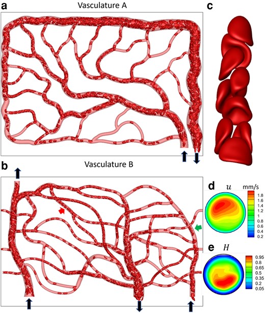
Data generation via high-fidelity RBC-resolved simulations. a and b) A visualization from the simulations for vasculature A and B. Black arrows indicate inlets/outlets. The images are in
The numerical methodology used in the high-fidelity simulations is based on a coupled finite volume/finite element/immersed-boundary method and is detailed in our previous studies (30, 43). Briefly, the in silico vasculatures are built using CAD software and contained in the computational domain that is discretized by
A visualization of the RBC distribution in one instant and a close-up of RBC shapes in a vessel segment are shown in Fig. 1a–c. Heterogeneous RBC distribution, which is a hallmark of the microvascular blood flow, is predicted in our simulation. Highly deformed RBC shapes, characterized as parachute and slipper shapes as observed in vivo, are also predicted.
The simulations provide 3D, time-resolved fluid velocity
ML models and results
Each vascular network is composed of three components: vessels, bifurcations, and mergers. The flow dynamics of RBCs and the mechanisms leading to complex velocity and hematocrit distributions in each vascular component are different. Thus, three separate ML modes are built for each component. Furthermore, the RBC concentration and blood velocity profiles are coupled together due to the coupling between RBC deformation and fluid motion, and hence, they must be predicted simultaneously.
We first build the ML models for each of the three vascular components using the DSR data from vasculature A. Then, we test the models and predict hemodynamic variables in vasculature B in two steps. First, we consider each vascular component in isolation: For example, for a bifurcation in vasculature B, we specify the DSR velocity and RBC concentration as the input immediately upstream of the bifurcation and predict the output at the daughter vessels immediately downstream. Next, we consider the entire vasculature-wide prediction. In this, we only specify the DSR data as the input at the inlet of the vasculature and predict the concentration and velocity profiles as they evolve in the entire vasculature by progressing through the hierarchy of vessels, bifurcations, and mergers.
Furthermore, we develop both 2D and 3D models. For the 2D model, the velocity and concentration distributions over the middle z plane of the network are considered so that
2D ML models
Bifurcations and Vessels and Mergers sections describe ML models for vascular components in isolation, and Vasculature-Wide Prediction section for the whole vasculature-wide prediction.
Bifurcations
The goal here is to predict the velocity and RBC concentration profiles in the daughter branches downstream of a bifurcation, namely,
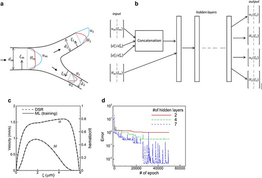
a) Schematic of the ML model and b) the structure of the ANN for a bifurcation. Notations are defined in the text. c) Comparison of the DSR and ML in the training process in a daughter vessel of one bifurcation in vasculature A. d) Convergence of training error for different numbers of hidden layers.
The DSR data is first prepared to generate the input and output vectors for training as
Additional input features required for the ML model are the ratio of the daughter to mother vessel cross-sectional area, i.e.
Figure 2b shows the ANN structure for the bifurcation. The inputs
A single ML model is developed using the data from all bifurcations in vasculature A. The training process starts with a randomly selected bifurcation and the loss function using mean squared error (MSE
Once the ML model is trained, we test it for each isolated bifurcation of vasculature B. For this, the DSR data in the mother vessel is used as the input. The model then predicts u and H profiles in the two daughter vessels as the output. Figure 3 shows a comparison of the ML-predicted profiles against the DSR data in three selected bifurcations. The agreement between them is excellent. An additional comparison is given in Fig. S2. The average MSE of the ML prediction is
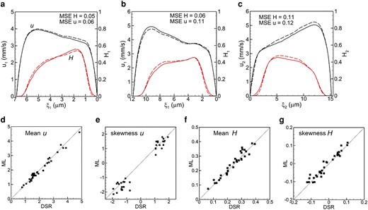
a–c) comparison of ML prediction and DSR data for three isolated bifurcations in 2d. Black curves are for u, and red for H. Dash curves represent ML and solid curves represent DSR. The mean and skewness of u and H profiles are compared in (d–g).
Vessels and mergers
Next, we build ML models for the remaining two vascular components, i.e. vessels and mergers. For vessels, the inputs are the velocity and concentration
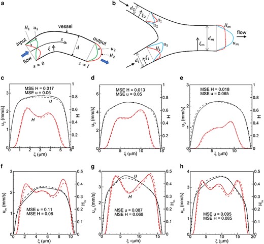
Schematic of the ML model for (a) vessels and (b) mergers. c–e) Predictions for vessels, and f–h) for mergers. Black represents velocity, and red hematocrit. Continuous curves are DSR data, and dash curves are ML prediction.
Figure 4c–e shows ML-predicted
Vasculature-wide prediction
We now test the models to make vasculature-wide predictions. For this, the DSR data is specified as input only at the vasculature inlet, and predictions are made sequentially through the hierarchy of the bifurcations, vessels, and mergers, with the prediction from one vascular component used as the input to the next component. Figure 5 compares the ML and DSR data at the end of two different paths that include multiple vascular components. Predictions along additional paths are given in Fig. S6. The MSE based on all vascular components in each path predicted is

Vasculature-wide 2D prediction following two different paths shown by arrows. ML and DSR results are compared at the end of the paths. Black and red colors represent u and H, respectively. Solid and dash curves represent DSR and ML prediction, respectively.
3D ML models
The 3D problem is schematically shown in Fig. 6a. Given
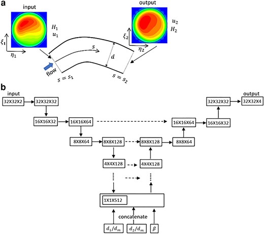
a) Schematic of 3D prediction. b) U-net model for a bifurcation. The left-hand side is the contraction (encoder) path, and the right side is the expansion (decoder) path. Each horizontal continuous arrow represents two consecutive convolutions, downward arrow represents max-pooling and upward arrow represents transposed convolutions. The horizontal dashed arrow represents concatenation of the output of the transposed convolution layers with the feature maps from the encoder.
Through numerical experiments, we found that at least
The U-net structure is shown in Fig. 6b for bifurcations. The encoder path is made of a sequential application of two consecutive regular convolutions using trainable filters of size 3×3 followed by a max-pooling which extracts the maximum value associated with a feature and reduces the size of the data. The down-sampling process continues until the data is flattened. Then a concatenation is performed to include geometric parameters, e.g.
Three U-net models corresponding to each vascular component are built. The nonlinear ReLU activation is used for all. A constant learning rate of
Figure 7 compares the ML prediction and DSR data for individual vessels, bifurcations, and mergers in isolation. Additional data are in Figs. S7–S9. The 3D predictions compare well against the DSR as the average of the mean absolute error (MAE) is
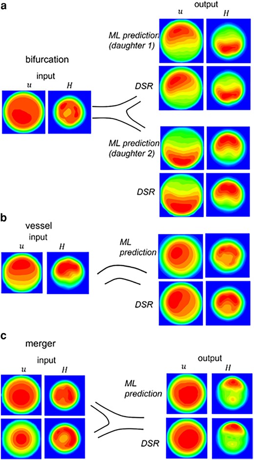
3D ML prediction in isolated bifurcations, vessels, and mergers. The left column is u and H at an upstream location used as input to the model. The right column is the output. The ML prediction is compared against the DSR data.
Figure 8 shows the vasculature-wide prediction using the 3D model. The ML and DSR results are compared at three locations along a selected path. Results for additional paths are given in Figs. S10–S12. In all cases, the MAE is 0.07—0.12 for
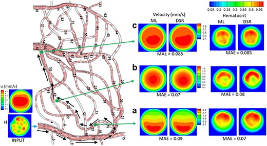
Vasculature-wide 3D prediction. Black arrows indicate the path. ML and DSR results are compared at three locations as marked by green arrows.
WSS and CFL
The WSS and CFL can be obtained from ML-predicted u and H and compared against the DSR data for each vascular component in isolation and for the vasculature-wide prediction, both in 2D and 3D (Figs. 9 and S10–S14). The WSS is obtained as the product of the radial gradient of u and plasma viscosity since the numerical stencil used to calculate the radial gradient is inside the near-wall CFL (21). The CFL is the distance from the wall where
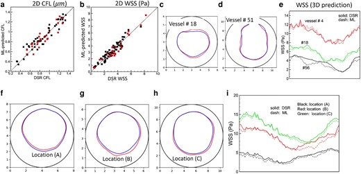
CFL and WSS prediction. a and b) 2D model. Black symbols: individual vascular component; red: vasculature-wide prediction along the paths shown in Fig. 5. c–e) 3D model for individual vascular components. f–i) 3D model for vasculature-wide prediction following the path shown in Fig. 8. The CFL and WSS are shown at three locations (A, B, C) as in that figure. In (c), (d) and (f)–(h) the interface between the plasm layer and RBC-core is shown in color (blue: DSR, red: ML), and the vessel boundary is indicated by black circle. The WSS in 3D prediction is shown along the circumference (horizontal axis in the plot) of the vessel. Numbering of the vessels is given in Figs. 8 and S1.
Timing comparison
In terms of computation time, the high-fidelity simulation of each vasculature took about 75,000 core-hours (wall-clock time × number of cores) on Intel Xeon Gold 6230 (Cascade Lake) CPUs to simulate one second of blood flow. In contrast, the training of the ML models took on average about seven hours on NVIDIA Tesla T4 GPU, and the predictions took only a few seconds. Additional few hours were also needed for data preparation. The ML models, therefore, reduce the time for hemodynamic prediction by several orders.
Discussions and conclusions
Existing imaging techniques of capillary vessel networks in vivo do not allow direct measurements of blood velocity and RBC concentration profiles over each vessel cross-section. Such information is needed to obtain physiologically important hemodynamic variables such as the WSS and CFL. High-fidelity, RBC-resolved simulations can provide such details, but they are computationally expensive. Here we presented ML models that can bypass such expensive computations but predict blood velocity and RBC concentration profiles in every vessel in a network. To train and test the models, we acquire data from high-fidelity simulations of deformable RBC suspension flowing in physiologically realistic in silico microvascular networks. A regression-type ANN model is used for 2D prediction, and a convolution-based U-net model is used for 3D. The models are first tested for individual vessels, bifurcations, and mergers. Thereafter, vasculature-wide predictions following different flow paths that involve multiple vascular components are considered. ML predictions compare against the high-fidelity simulation data with
The time taken by the ML models to predict the hemodynamic quantities in the networks considered here is found to be several orders less than that of the high-fidelity model. Indeed, the high-fidelity models are based on fundamental principles, provide a large amount of information, and reveal new physics. In many applications, only a few, specific hemodynamic variables may be of interest and the discovery of new physics is not intended. An example is the WSS distribution in a network which is often the intended hemodynamic variable. In such situations, the high-fidelity model can be avoided, and the ML models, instead, can be used to provide highly accurate, detailed data. The high-fidelity models also require high-performance computing resources and specific expertise of the user, whereas the ML models can be run on web-based platforms and by users with wider domain expertise.
The vasculatures used here span over relatively smaller tissue regions compared to what current in vivo imaging techniques can map at an organ-scale, e.g. the human retina (5), and whole mouse brain (23). Detailed and accurate hemodynamic quantities in such massive networks would be useful, for example in understanding the progression of retinopathy, Alzheimer's disease, and dementia, but cannot be feasibly obtained from high-fidelity simulations. In contrast, the significant reduction in the prediction time makes the ML models highly viable for this.
Although the present ML models are trained and tested using simulated RBC flow in microvasculature in silico, they can also be used for predictions using in vivo images and experimental data. Since simultaneously imaging the vasculature and measuring the profiles of RBC concentration and blood velocity is not possible, the ML models presented here can be an effective tool that can accurately predict detailed, 3D hemodynamic parameters in every vessel of the in vivo networks. Remarkably, using the current ML “bank”, the models can be used to predict hemodynamics in the entire vasculature that could consist of a large number of vessels and vascular junctions. It also implies that in complex vascular topologies, for which some hemodynamic information may be missing, the ML model can be applied to fill such voids. Also, the approach is generalizable to multiple inlets as is the case for the testing vasculature used here. If several inlets act as arteries, the vessel and bifurcation models can be applied sequentially to each of them. If several of the inlets are veins, the vessel and merger models can also be applied sequentially.
As in any ML application, the error reduces with an increasing amount of training data. The amount of data used here is deemed to be modest. Furthermore, the error depends on how closely the training and testing vasculatures match in terms of both their geometry and controlling hemodynamic parameters, such as flow rate and vessel hematocrit. The distribution of vessel diameter over successive generations generally follows Horton's law (2) which provides some sort of commonality of the topology in two vasculatures. However, when compared at the level of individual vascular components, there are differences between the two networks. These competing factors resulted in varying accuracy between different vessels. The availability of additional training data spanning a larger parameter space, both in terms of geometry and controlling flow parameters, will reduce the error. Furthermore, for the vasculature-wide prediction, continuous growth of error is not observed, implying that a limited number of trained models can be used for predictions in large networks. If the geometry and flow conditions are very different in two networks, then the error will be high. Also, both vasculatures have similar number of vascular components and span over similar tissue area. If the testing vasculature has a lot more vascular components that differ from the training vasculature, the error is expected to grow.
Some limitations of the current ML models can be noted. The vessels considered here are cylindrical and have constant diameter. As such, the ML model as presented here is not applicable to noncircular vessels and those with changing diameters both of which can affect
The current ML models are not physics-informed models. No explicit physical constraint was imposed. The model tries to learn the physics from the DSR data which obeys the conservation laws. The models are constructed such that the inputs, e.g. u, H, and d, enable to preserve the flow rate and RBC flux. We did not see any loss in such conserved quantities except one or two bifurcations which have very different geometry and flow conditions compared to the training vasculature.
The current ML models, which to our knowledge are the first of their kind, are highly promising for image-based predictions of subcellular resolved capillary hemodynamics in organ-scale networks (24, 26). ML models following the same techniques presented here can be built for predicting hemodynamics in blood cell disorders, such as sickle cell anemia, malaria, and diabetes mellitus, that are characterized by reduced RBC deformability (6, 7, 45, 46). They can also be used to predict transport of biomolecules and drugs in diseased vasculature, e.g. tumor microvasculature (8, 9). Further extensions can predict altered hemodynamics during vascular adaptation, e.g. during embryonic development, angiogenesis, vasculopathy, and cerebrovascular dysfunction. They can also be applied to nonbiological applications, such as fluids and tracer transport in porous media resolved with pore-scale details.
Acknowledgments
Computational resources at Pittsburgh Supercomputing Center, Texas Advanced Computing Center, and Rutgers University are acknowledged.
Supplementary Material
Supplementary material is available at PNAS Nexus online.
Funding
This work was supported by a grant from the National Institute of Health (R01EY033003) and National Science Foundation (CBET-2302212).
Author Contributions
P.B. designed the research and wrote the paper. S.E. designed research, developed code, performed simulations, analyzed data, and wrote the paper.
Data Availability
Data, code, and documentation are available in Github and can be downloaded from https://github.com/SamEbiRutgers/ML_Microvasculature.git.
References
Author notes
Competing Interest: The authors declare no competing interest.