Abstract
Spontaneous synchronization is ubiquitous in natural and man-made systems. It underlies emergent behaviors such as neuronal response modulation and is fundamental to the coordination of robot swarms and autonomous vehicle fleets. Due to its simplicity and physical interpretability, pulse-coupled oscillators has emerged as one of the standard models for synchronization. However, existing analytical results for this model assume ideal conditions, including homogeneous oscillator frequencies and negligible coupling delays, as well as strict requirements on the initial phase distribution and the network topology. Using reinforcement learning, we obtain an optimal pulse-interaction mechanism (encoded in phase response function) that optimizes the probability of synchronization even in the presence of nonideal conditions. For small oscillator heterogeneities and propagation delays, we propose a heuristic formula for highly effective phase response functions that can be applied to general networks and unrestricted initial phase distributions. This allows us to bypass the need to relearn the phase response function for every new network.
Editor:
Derek Abbott
Search for other works by this author on:
Significance StatementDue to its simplicity and physical interpretability, pulse-coupled oscillators has emerged as one of the standard models to study synchronization in both biological and engineered networks. However, finding an optimal pulse-interaction mechanism is challenging, and generally intractable in practical scenarios involving random delays and frequency differences. By utilizing reinforcement learning strategies, we obtain pulse-interaction mechanisms that optimize both the speed and probability of synchronization even in the presence of random delays and frequency differences. The results give a general formula of the optimal interaction mechanism for arbitrary network structures, and hence enables predicting the optimal interaction mechanism for every new network without re-implementing the reinforcement learning process.
Introduction
Recent research has turned to using the pulse-coupled oscillator (PCO) model (1–10) that was initially proposed to describe biological neuronal networks (11–22) and cardiac pacemakers (23–26), but has subsequently found applications in many other systems, including artificial neural networks (27), social self-organization (28), and clock coordination of wireless sensor networks (29, 30). The PCO model explicitly incorporates the hybrid nature of network dynamics (in contrast to other models such as the Kuramoto oscillators (31)) and promises great potential for synchronizing engineered networks (29). For example, the PCO-based strategies have been found to be highly successful in achieving motion coordination in robot swarms (32–34). Since only simple and content-free pulses are sent between agents, PCO-based synchronization is naturally resilient to message corruption in communications and incurs little communication overhead, leading to improved network robustness and reduced communication latency (35, 36). These advantages make PCO-based synchronization particularly appealing for the coordination in engineering networks such as robot swarms and vehicle fleets that are subject to stringent reliability and real-time constraints.
The synchronizability of PCO networks depends crucially on the phase response function (PRF), which characterizes how an oscillator adjusts its phase when a pulse is received from a neighboring oscillator (37). The amount of adjustment depends on the current state of the receiving oscillator. Many analytical results on PRF have been reported under ideal conditions. For example, Klinglmayr et al. (38) and Lyu (39) investigated the synchronization of PCOs with stochastic PRFs. Lyu (40) further analyzed the synchronization time of PCOs on tree networks. Wang and Doyle (41) proposed a PRF that can maximize the speed of synchronization of PCOs when the initial oscillator phases are distributed within a half-cycle. However, these results are often obtained under ideal conditions, including zero time delays and identical oscillator frequencies. In fact, nonideal factors such as propagation delays and heterogeneous oscillator frequencies render the analytical design of PRF extremely difficult, if at all possible (9, 42–49, 50–52).
In this article, we propose a reinforcement learning (RL) approach to determine a highly effective PRF under both ideal and nonideal conditions. The interaction strategy found by our RL approach improves synchronization probability compared to previously proposed PRFs in (41, 42, 43, 47). Moreover, our results provide insights on a general design principle for PRF that can be adapted to general network topologies. Finally, the flexibility of our RL framework allows oscillators to adapt to changing network structures and environmental noise, ensuring robust synchronization under real-world conditions.
Results
Pulse-coupled oscillators
Let us consider a network of N PCOs, where is the phase of oscillator . Each oscillator evolves its phase at a frequency . When reaches the threshold value , oscillator i fires a pulse and resets its phase to zero. Neighboring oscillators receive this pulse after some (random) time delay . This delay in receiving a pulse is primarily due to the finite propagation speed of the pulse, but it may also include the time required for a node to process the incoming pulse.
An oscillator responds to a received pulse by changing its phase by
where and represent the phase of oscillator i immediately before and after receiving a pulse, respectively. The function , which determines the amount that an oscillator will adjust its phase as a function of its phase value upon which the pulse is received, is called the phase response function (PRF). The jump in the value of the phase is determined not only by the PRF, but also by the coupling strength , which is introduced to facilitate the analysis and design of PCO-based synchronization in engineered systems (41, 42, 49, 53). It is worth noting that PRF is related to the phase transition curve (PTC) in (43) as .
To quantify the degree of synchronization of an oscillator network, we define the containing arc as the smallest interval in that contains all oscillator phases in the network:
Following (54), we define an arc as a connected subset of the one dimension torus . Thus, in the preceding Eq. (2) denotes the length of the arc along to the first oscillator ahead in the phase of oscillator i. Note that always holds. Hence, is the smallest arc containing all oscillators and can be used to quantify the degree of synchronization.
We use RL to determine an optimal PRF that maximizes the probability of synchronization for a given number of oscillators:
where G is an underlying graph with edges drawn randomly according to some distribution, is an initial phase configuration drawn uniformly at random, and is the phase trajectories of all oscillators under a given PRF and initial phase distribution.
Reinforcement learning
A number of works have recently been reported that use learning methods to investigate the dynamics of coupled oscillators (see, e.g. 55–58). However, all of these results consider smooth-interaction oscillators like Kuramoto oscillators. Recently the authors of (59) propose to use learning methods to predict if an oscillator network can synchronize or not, and they consider both smooth and pulse interactions. The approach in (59) considers interaction mechanisms that are given and predetermined. In this work, we leverage the exploration and adaptation properties of RL to optimize the interaction mechanism of PCOs. More specifically, we use RL to determine an optimal PRF that maximizes the probability to synchronize under both ideal and nonideal conditions. It is worth noting that formal analysis of PCO networks under general initial phase distributions and practical nonideal conditions, such as coupling delay and frequency heterogeneity, remains out of reach with current analytic techniques (47, 60). With RL strategies, we can model the nonideal factors, and let the oscillators evolve naturally in the network and gradually optimize their response to maximize synchronization probability.
A schematic of the approach is given in Fig. 1. Specifically, for each oscillator , the state is its phase value . When a pulse is received from a neighboring oscillator, oscillator i changes its phase value by an action . The value of each possible state-action pair is described as a matrix . Based on the current state-action values, oscillator i chooses a policy under its environment, which consists of its neighboring oscillators along with the network dynamics. Each oscillator receives a set of reward values, which are used to update the state-action values. The RL process repeats until an optimal policy is obtained. By taking the average of , we find a best piece-wise linear fit as the optimal PRF. The detailed RL protocol, such as the designs of reward values and Q-value update are described in the “Materials and Methods” section.
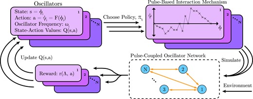
Fig. 1.
Schematic of the reinforcement learning framework proposed for pulse-coupled oscillators.
Optimal phase response functions under ideal conditions
We first consider the ideal case where oscillators have identical frequency and pulses are received instantaneously with no delay. We begin with a PCO network of oscillators, where the containing arc is always within a half of a cycle. Fig. 2 shows the average learned policy over 10 experiments, which closely approximates the proposed PRF in (41) obtained analytically under the assumption that the containing arc is less than half of a cycle:
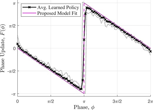
Fig. 2.
Average optimal policy learned using a network of two oscillators with identical frequencies and zero delay. The dotted lines show the maximum variations in the learned policies. The learned PRF closely approximates the analytical solution in (41).
We next consider oscillators with all-to-all coupling (more results for , 4, 5 and ER random graphs see Fig. S1–S6 in the supplementary materials). Fig. 3 shows the optimal average learned policy over 18 experiments, which is different from the analytical result in (41), primarily due to the unrestricted phase distributions. During the training phase, the randomness in the policy selection does not guarantee that the oscillators stay within a half-cycle,even if the phase values were initialized within a half-cycle. Thus, the assumptions for the analytical result in (41) do not hold in this case.
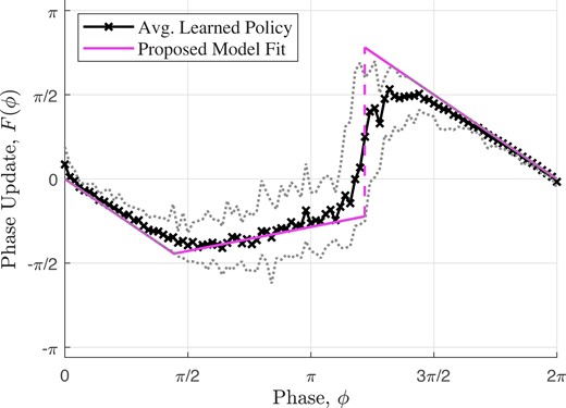
Fig. 3.
Average optimal policy learned using six oscillators in an all-to-all topology with identical frequencies and zero delay. The dotted lines show the maximum variations in the learned policies. Since the oscillators can have an unrestricted distribution of initial phases, the learned PRF is significantly different from the analytical prediction in (41) and is better modeled using Eq. (5).
Design principle of phase response functions
The average learned policies from both Figs. 2 and 3 can be modeled using a simple form
where and are positive constants that will be determined later. The best-fits to the learned policies using Eq. (5) are shown in Figs. 2 and 3.
This PRF model offers important insight into the design principles of the highly effective phase response policy. When its phase value is close to the start or end of a cycle, an oscillator learns to take the maximum phase adjustment toward the threshold value, which has been shown analytically to decrease the synchronization time in (41). But when the phase value is near the middle of the cycle, the oscillator adjusts its phase proportionally to the distance to the end of the cycle, similar to the strategy used in (43), which has been shown to almost always lead to synchronization. This combination of two different strategies gives a phase response function that achieves synchronization efficiently.
We now use Erdős–Rényi–Gilbert (ERG) networks with parameters chosen at random to find the best parameters for Eq. (5). Fig. 4 shows the best-fit values for the parameters and , which fit well to exponential functions of the oscillator indegree :
where and are constants. This formula reduces the optimization of a function to the much simpler problem of optimizing two parameters. Equation (5) combined with Eq. (6) provides a powerful heuristic formula that can be used to predict the optimal PRF for oscillators in general networks without repeating the RL process.
![Training and test data from best-fit values of learned phase response functions. The training data show the average and range of the best-fit values of the function parameters c1 and c2 in Eq. (5) to the optimal average learned policy of all oscillators on Erdős–Rényi–Gilbert (ERG) networks G(n,p) with n and p generated randomly in the intervals [6,25] and (0,1), respectively (discarding network realization that are not connected). It is also used to determine the best-fit exponential curve given by Eq. (6) for each function parameter. The testing data show the best-fit values of the function parameters for each oscillator in Watts-Strogatz networks G(N,K,β), where N=50, β=1, and K is varied from 1 to 25. Oscillators with identical indegree learn similar PRFs of the form given by Eq. (5) with similar learned function parameter values that are well-predicted by Eq. (6), regardless of network size or topology.](https://oup.silverchair-cdn.com/oup/backfile/Content_public/Journal/pnasnexus/2/4/10.1093_pnasnexus_pgad102/3/m_pgad102f4.jpeg?Expires=1747925380&Signature=jR8E8jaxyC7F4NefcbCFLA8pULaTpCou2wGJjxioOKDNtkZurMoxZhfrXRmEPD0CeDO0NfKGn8NMPFReFlgk0qdzva4Fiq~GtZhM~DeybDnAEoUdz9m8XJfkYRWAX8knbB0q0cYUQBLmDqoJEl6~nDJLIMw3dbWLRDBs6FqDTu3shoqEKVeXq~b9uFtbnDUS-YMz9tfwhdqFtAKC-f-8jBWK81P5~lXF3wJDg~VbruFVTGAPXukEDaBRdxGO1qFnd6ALlskA501r8rMLvEbbdaHMo7n2C9UdHmXljVd3ytZLp~ROh67ei259mK0S86n5NHu8iU77~DckpH6BEO5GsQ__&Key-Pair-Id=APKAIE5G5CRDK6RD3PGA)
Fig. 4.
Training and test data from best-fit values of learned phase response functions. The training data show the average and range of the best-fit values of the function parameters and in Eq. (5) to the optimal average learned policy of all oscillators on Erdős–Rényi–Gilbert (ERG) networks with n and p generated randomly in the intervals and , respectively (discarding network realization that are not connected). It is also used to determine the best-fit exponential curve given by Eq. (6) for each function parameter. The testing data show the best-fit values of the function parameters for each oscillator in Watts-Strogatz networks , where , , and K is varied from 1 to 25. Oscillators with identical indegree learn similar PRFs of the form given by Eq. (5) with similar learned function parameter values that are well-predicted by Eq. (6), regardless of network size or topology.
Optimal phase response functions under nonideal conditions
When we consider experiments using various nonidentical oscillator frequencies (with differences within of the nominal frequency) and nonzero propagation delays (with delays within of an oscillation cycle), we find that learned PRFs are very similar to the ones for ideal environments (see Fig. S7–S14 in the supplementary materials for more details). Thus, we conclude that the same PRFs are optimal in achieving synchronization when the network is subject to moderate nonideal conditions.
Next, we compare our learned PRF based on Eq. (5) to previously proposed PRFs in (41, 42, 43, 47) under nonideal conditions. Since the synchronization strategies by Mirollo and Strogatz (43), Nishimura and Friedman (47), and Klinglmayr (42) do not include an explicit coupling strength parameter, we modify these algorithms to scale the change in phase adjustment by the coupling strength l, as in Eq. (1). These algorithms are recovered under .
For our test, we consider an ER random graph with oscillators and edge probability , as illustrated in Fig. 5. We set the oscillator frequency uniformly distributed in the range and propagation delays uniformly distributed in the range cycles. We randomly assign initial oscillator phase values in .
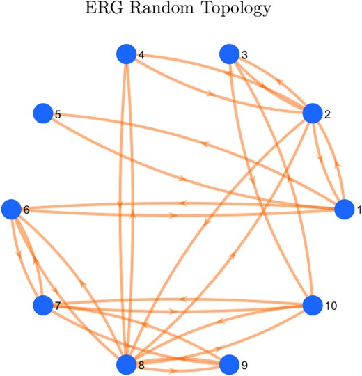
Fig. 5.
The Erdős–Rényi–Gilbert (ERG) graph used in Figs. 6 and 7 for the comparison between our learned PRF and previously proposed PRFs.
Fig. 6 shows the average value of the containing arc at steady-state after 2,000 runs over a broad range of coupling strength values. Our learned PRF, Wang and Doyle’s delay-advance PRF in (41), and Nishimura and Friedman’s “strong type II” PRF in (47) are able to synchronize the network more closely than the other synchronization strategies due to the similarity among these PRFs. The addition of the coupling strength parameter allows for additional tuning to achieve a greater level of synchronization, especially in nonideal environments.
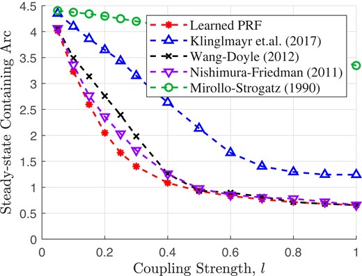
Fig. 6.
Average of the steady-state containing arc for ten oscillators in an ER random topology (Fig. 5) with nonidentical oscillator frequencies and random coupling delays.
Moreover, if we look at how often the network is able to synchronize, we see that our learned PRF is able to synchronize more often at low coupling strengths than any of the other synchronization strategies, as shown in Fig. 7. Similar results are obtained when we vary the network size and topology, the amount of oscillator frequency heterogeneity, and the amount of coupling delay (see Figs. S15–S25 in the supplementary materials for more details).
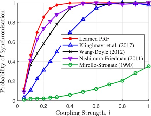
Fig. 7.
Probability of synchronizing ten oscillators in an ER random topology (Fig. 5) with nonidentical frequencies and random delay. The learned PRF is able to synchronize more frequently than the other strategies, especially for smaller coupling strengths.
Discussion
The proposed reinforcement learning framework provides a simple and versatile method for optimizing synchronization in pulse-coupled oscillator networks to maximize the degree and resilience of synchronization. Given that maintaining synchronization in the presence of message corruption and communication delays is crucial for numerous systems and processes, the results are expected to have broad applications in biological and engineered systems. For example, biological systems such as cardiac pacemakers and neuron networks can be effectively modeled by PCOs (61). In addition, the proposed method are well positioned to synchronize clocks in wireless sensor networks (41, 42, 53) and coordinate motions in robot networks (32, 34). Furthermore, to the best of our knowledge, this paper is the first to use a distributed reinforcement learning approach to optimize synchronization under noncontinuous pulse-based interactions, which is different from continuous-time smooth interactions in the Kuramoto model (62). It has direct ramifications for the deployment of reinforcement learning in general multiagent systems to optimize dynamical processes in general networks.
Future works include minimizing the synchronization time for PCOs and incorporating mechanisms to allow oscillators to adapt their intrinsic frequencies to deal with large frequency heterogeneity. Further improvements in the design of reward values, along with expanded action space (e.g. allow adjustments of both oscillator phases and frequencies), may lead to better control of both synchronization and desynchronization in networks of sensors and robots with discrete-time.
Materials and methods
Reinforcement learning protocol
State, action, and Q-value
Since the oscillator’s state and action values evolve on continuous intervals, parameterization and approximation decisions must be made to implement RL. We parameterize the continuous state interval into evenly spaced parameters, . The state parameter corresponds to the phase value in . Additionally, we discretize the actions with values, , such that the actions are limited to phase changes that keep the oscillator within its current cycle. The possible actions that can be taken by an oscillator for can be expressed as for . We represent the value of each state-action pair with a matrix . Each element of estimates the amount of expected reward by taking the action a at state s.
We implement episodic RL using an on-policy temporal-difference RL technique (see, e.g. 63). Off-policy RL techniques, such as Q-learning, tend to perform worse when there is a need to approximate continuous states and action spaces based on (64). A policy π for our MDP consists of a set of actions, one action for each state parameter , such that . This policy represents a straight-line approximation of the PRF for an oscillator . For on-policy learning, we choose a policy before each episode. To avoid confusion with phase , we denote policies with subscripts, such that the policy used for episode t is . The choice for a policy is based on the current state-action value estimates . We use a soft-max, or Boltzmann, distribution to choose an action. Initially, the values for all state-action pairs are set to zero. Thus, the initial policy is equally likely to choose any action.
Reward design
Our goal is to have the oscillators synchronize their phases. Due to the dynamics of PCO networks, the choice of reward and how to update the values of state-action pairs are both critical. Since the length of the containing arc measures how well the network is synchronized, we reward actions that decrease the length of the containing arc and penalize actions that increase that length. Thus, the reward will include the decrease in the length of the containing arc, , where and are the lengths of the containing arc before and after the action was taken, respectively.
Individual oscillators in a PCO network do not know the true state of the network. However, each oscillator can approximately estimate the state of the network by keeping track of the phase differences between itself and other oscillators when a pulse is received. Therefore, we can use the oscillator’s estimated state to approximate the change in the containing arc and, thus, determine the reward value.
Multiple actions can result in the same decrease in the containing arc. To encourage efficient synchronization, we penalize the oscillator by based on the magnitude of the action . Therefore, when an oscillator receives its kth pulse and takes an action that decreases the (estimated) containing arc by an amount , the total reward is given by
where and are positive weights.
During a training episode t, we let the network evolve for a fixed amount of time following a given policy . When an oscillator receives a pulse, it uses to determine its action, i.e. phase adjustment, based on a given coupling strength l and its current phase .
Let us denote the two closest state parameters to for the kth received pulse as and , respectively, where holds. The corresponding actions from policy for those state parameters are denoted as and , respectively. To determine the action that the oscillator takes, we weight the actions of the two nearest state parameters based on the proximity of the current phase to those state variables. That is, the phase adjustment in Eq. (1) is
with and .
Before an oscillator adjusts its phase, it records its current state as , where k is an index for the number of received pulses during an episode. The action taken, based on the policy , is recorded as . The oscillator calculates its reward based on Eq. (7) and then evolves freely until another pulse is received.
Q-value update
Once an episode for the network is complete, we use the resulting state-action-reward sequences to perform a batch update of the state-actions value matrix . The update is based on the Sarsa algorithm in (64), where the reward will apply to the state-action values for the two nearest state parameters to and their corresponding actions from the episode policy . The update for is
and the update for is
where α is the learning rate and γ is the discount rate. Here, denotes the average estimated value of the next state-action pair () and is calculated as
This update is performed for every state-action pair except for the final pair, which is the terminal state.
After all updates have been completed for each oscillator’s state-action-reward sequence, an episode of training is complete. With the updated state-action value matrix , a new policy is chosen for the next episode, and the process is repeated. After all episodes of training are complete, we use to determine the optimal policy , where for each state parameter . We note that different oscillators in a network can have different optimal policies .
In the implementation, for each case, we let the network evolve for 15 cycles for each episode with initial phases randomly selected in , and use a coupling strength . We parameterize the state with 101 evenly spaced parameters and discretize the policy actions into 201 evenly spaced values. For each experiment, we simulate a network for 100,000 episodes. We use and for Eq. (7).
Acknowledgments
We thank Steven Strogatz for helpful discussions.
Supplementary Material
Supplementary material is available at PNAS Nexus online.
Funding
The work was supported in part by the National Science Foundation under Grant 2012075.
Authors’ Contribution
T.A. and Y. W. conceived the project. Z.C, T.A., and Y.W. performed the research. Z.C, T.A., Y.Z. and Y.W. discussed the results. Z.C, T.A., Y.Z. and Y.W. wrote the paper.
Data Availability
All data is included in the manuscript and/or supporting information.
References
1
Abbott
LF
,
van Vreeswijk
C
.
1993
.
Asynchronous states in networks of pulse-coupled oscillators
.
Phys Rev E
.
48
:
1483
.
2
Timme
M
,
Wolf
F
,
Geisel
T
.
2002
.
Coexistence of regular and irregular dynamics in complex networks of pulse-coupled oscillators
.
Phys Rev Lett
.
89
:
258701
.
3
Timme
M
,
Wolf
F
,
Geisel
T
.
2002
.
Prevalence of unstable attractors in networks of pulse-coupled oscillators
.
Phys Rev Lett
.
89
:
154105
.
4
Timme
M
,
Wolf
F
,
Geisel
T
.
2004
.
Topological speed limits to network synchronization
.
Phys Rev Lett
.
92
:
074101
.
5
Pazó
D
,
Montbrió
E
.
2014
.
Low-dimensional dynamics of populations of pulse-coupled oscillators
.
Phys Rev X
.
4
:
011009
.
6
Dörfler
F
,
Bullo
F
.
2014
.
Synchronization in complex networks of phase oscillators: a survey
.
Automatica
.
50
:
1539
–
1564
.
7
O’Keeffe
KP
,
Krapivsky
PL
,
Strogatz
SH
.
2015
.
Synchronization as aggregation: cluster kinetics of pulse-coupled oscillators
.
Phys Rev Lett
.
115
:
064101
.
8
Kannapan
D
,
Bullo
F
.
2016
.
Synchronization in pulse-coupled oscillators with delayed excitatory/inhibitory coupling
.
SIAM J Control Optim
.
54
:
1872
–
1894
.
9
Vogell
A
,
Schilcher
U
,
Bettstetter
C
.
2020
.
Deadlocks in the synchronization of pulse-coupled oscillators on star graphs
.
Phys Rev E
.
102
:
062211
.
10
Righetti
L
,
Buchli
J
,
Ijspeert
AJ
.
2006
.
Dynamic Hebbian learning in adaptive frequency oscillators
.
Physica D
.
216
:
269
–
281
.
11
Bartos
M
,
Vida
I
,
Jonas
P
.
2007
.
Synaptic mechanisms of synchronized gamma oscillations in inhibitory interneuron networks
.
Nat Rev Neurosci
.
8
:
45
–
56
.
12
Pervouchine
DD
, et al.
2006
.
Low-dimensional maps encoding dynamics in entorhinal cortex and hippocampus
.
Neural Comput
.
18
:
2617
–
2650
.
13
Timme
M
,
Wolf
F
.
2008
.
The simplest problem in the collective dynamics of neural networks: is synchrony stable?
Nonlinearity
.
21
:
1579
.
14
Canavier
CC
,
Achuthan
S
.
2010
.
Pulse coupled oscillators and the phase resetting curve
.
Math Biosci
.
226
:
77
–
96
.
15
Ding
Y
,
Ermentrout
B
.
2021
.
Traveling waves in non-local pulse-coupled networks
.
J Math Biol
.
82
:
1
–
20
.
16
Bolhasani
E
,
Valizadeh
A
.
2015
.
Stabilizing synchrony by inhomogeneity
.
Sci Rep
.
5
:
13854
.
17
Smeal
RM
,
Ermentrout
GB
,
White
JA
.
2010
.
Phase-response curves and synchronized neural networks
.
Philos Trans R Soc Lond B Biol Sci
.
365
:
2407
–
2422
.
18
Stiefel
KM
,
Ermentrout
GB
.
2016
.
Neurons as oscillators
.
J Neurophysiol
.
116
:
32950
–
2960
.
19
Burton
SD
,
Ermentrout
GB
,
Urban
NN
.
2012
.
Intrinsic heterogeneity in oscillatory dynamics limits correlation-induced neural synchronization
.
J Neurophysiol
.
108
:
2115
–
2133
.
20
Canavier
CC
,
Wang
S
,
Chandrasekaran
L
.
2013
.
Effect of phase response curve skew on synchronization with and without conduction delays
.
Front Neural Circuits
.
7
:
194
.
21
Abouzeid
A
,
Ermentrout
B
.
2009
.
Type-II phase resetting curve is optimal for stochastic synchrony
.
Phys Rev E
.
80
:
011911
.
22
Ermentrout
B
.
1991
.
An adaptive model for synchrony in the firefly Pteroptyx malaccae
.
J Math Biol
.
29
:
571
–
585
.
23
Bell-Pedersen
D
, et al.
2005
.
Circadian rhythms from multiple oscillators: lessons from diverse organisms
.
Nat Rev Genet
.
6
:
544
–
556
.
24
Peskin
CS
.
1975
.
Mathematical aspects of heart physiology
.
NYU’s Courant Inst. Math
.
25
Ly
C
,
Weinberg
SH
.
2018
.
Analysis of heterogeneous cardiac pacemaker tissue models and traveling wave dynamics
.
J Theor Biol
.
459
:
18
–
35
.
26
Nakano
K
,
Nanri
N
,
Tsukamoto
Y
,
Akashi
M
.
2021
.
Mechanical activities of self-beating cardiomyocyte aggregates under mechanical compression
.
Sci Rep
.
11
:
15159
.
27
Vidal
J
,
Haggerty
J
.
1987
.
28
Néda
Z
,
Ravasz
E
,
Brechet
Y
,
Vicsek
T
,
Barabási
A-L
.
2000
.
The sound of many hands clapping
.
Nature
.
403
:
849
–
850
.
29
Sundararaman
B
,
Buy
U
,
Kshemkalyani
AD
.
2005
.
Clock synchronization for wireless sensor networks: a survey
.
Ad Hoc Netw
.
3
:
281
–
323
.
30
Silvestre
D
,
Hespanha
J
,
Silvestre
C
.
2019
. .
31
O’Keeffe
KP
,
Hong
H
,
Strogatz
SH
.
2017
.
Oscillators that sync and swarm
.
Nat Commun
.
8
:
1
–
13
.
32
Gao
H
,
Wang
Y
.
2018
.
A pulse-based integrated communication and control design for decentralized collective motion coordination
.
IEEE Trans Automat Control
.
63
:
1858
–
1864
.
33
Barciś
A
,
Bettstetter
C
.
2020
.
Sandsbots: robots that sync and swarm
.
IEEE Access
.
8
:
218752
–
218764
.
34
Anglea
T
,
Wang
Y
.
2019
.
Decentralized heading control with rate constraints using pulse-coupled oscillators
.
IEEE Trans Control Netw Syst
.
7
:
1090
–
1102
.
35
Wang
Z
,
Wang
Y
.
2018
.
Pulse-coupled oscillators resilient to stealthy attacks
.
IEEE Trans Signal Process
.
66
:
3086
–
3099
.
36
Wang
Z
,
Wang
Y
.
2020
.
An attack-resilient pulse-based synchronization strategy for general connected topologies
.
IEEE Trans Automat Control
.
65
:
3784
–
3799
.
37
Stankovski
T
,
Pereira
T
,
McClintock
PV
,
Stefanovska
A
.
2017
.
Coupling functions: universal insights into dynamical interaction mechanisms
.
Rev Mod Phys
.
89
:
045001
.
38
Klinglmayr
J
,
Kirst
C
,
Bettstetter
C
,
Timme
M
.
2012
.
Guaranteeing global synchronization in networks with stochastic interactions
.
New J Phys
.
14
:
073031
.
39
Lyu
H
.
2015
.
Synchronization of finite-state pulse-coupled oscillators
.
Physica D
.
303
:
28
–
38
.
40
Lyu
H
.
2018
.
Global synchronization of pulse-coupled oscillators on trees
.
SIAM J Appl Dyn Syst
.
17
:
1521
–
1559
.
41
Wang
Y
,
Doyle III
FJ
.
2012
.
Optimal phase response functions for fast pulse-coupled synchronization in wireless sensor networks
.
IEEE Trans Signal Process
.
60
:
5583
–
5588
.
42
Klinglmayr
J
,
Bettstetter
C
,
Timme
M
,
Kirst
C
.
2017
.
Convergence of self-organizing pulse-coupled oscillator synchronization in dynamic networks
.
IEEE Trans Automat Control
.
62
:
1606
–
1619
.
43
Mirollo
R
,
Strogatz
S
.
1990
.
Synchronization of pulse-coupled biological oscillators
.
SIAM J Appl Math
.
50
:
1645
–
1662
.
44
Ernst
U
,
Pawelzik
K
,
Geisel
T
.
1995
.
Synchronization induced by temporal delays in pulse-coupled oscillators
.
Phys Rev Lett
.
74
:
1570
.
45
Goel
P
,
Ermentrout
B
.
2002
.
Synchrony, stability, and firing patterns in pulse-coupled oscillators
.
Physica D
.
163
:
191
–
216
.
46
Zeitler
M
,
Daffertshofer
A
,
Gielen
CCAM
.
2009
.
Asymmetry in pulse-coupled oscillators with delay
.
Phys Rev E
.
79
:
065203
.
47
Nishimura
J
,
Friedman
EJ
.
2011
.
Robust convergence in pulse-coupled oscillators with delays
.
Phys Rev Lett
.
106
:
194101
.
48
Nishimura
J
,
Friedman
EJ
.
2012
.
Probabilistic convergence guarantees for type-II pulse-coupled oscillators
.
Phys Rev E
.
86
:
025201
.
49
Núñez
F
,
Wang
Y
,
Doyle III
FJ
.
2015
.
Synchronization of pulse-coupled oscillators on (strongly) connected graphs
.
IEEE Trans Automat Control
.
60
:
1710
–
1715
.
50
Hata
S
,
Arai
K
,
Galán
RF
,
Nakao
H
.
2011
.
Optimal phase response curves for stochastic synchronization of limit-cycle oscillators by common poisson noise
.
Phys Rev E
.
84
:
016229
.
51
Harada
T
,
Tanaka
HA
,
Hankins
MJ
,
Kiss
IZ
.
2010
.
Optimal waveform for the entrainment of a weakly forced oscillator
.
Phys Rev Lett
.
105
:
088301
.
52
Pfeuty
B
,
Thommen
Q
,
Lefranc
M
.
2011
.
Robust entrainment of circadian oscillators requires specific phase response curves
.
Biophys J
.
100
:
2557
–
2565
.
53
Wang
Y
,
Nunez
F
,
Doyle
FJ
.
2012
.
Energy-efficient pulse-coupled synchronization strategy design for wireless sensor networks through reduced idle listening
.
IEEE Trans Signal Process
.
60
:
5293
–
5306
.
54
Núñez
F
,
Wang
Y
,
Teel
AR
,
Doyle III
FJ
.
2016
.
Synchronization of pulse-coupled oscillators to a global pacemaker
.
Syst Control Lett
.
88
:
75
–
80
.
55
Fan
H
,
Kong
LW
,
Lai
YC
,
Wang
X
.
2021
.
Anticipating synchronization with machine learning
.
Phys Rev Res
.
3
:
023237
.
56
Guth
S
,
Sapsis
TP
.
2019
.
Machine learning predictors of extreme events occurring in complex dynamical systems
.
Entropy
.
21
:
925
.
57
Chowdhury
SN
,
Ray
A
,
Mishra
A
,
Ghosh
D
.
2021
.
Extreme events in globally coupled chaotic maps
.
J Phys Complex
.
2
:
035021
.
58
Thiem
TN
,
Kooshkbaghi
M
,
Bertalan
T
,
Laing
CR
,
Kevrekidis
IG
.
2020
.
Emergent spaces for coupled oscillators
.
Front Comput Neurosci
.
14
:
36
.
59
Bassi
H
, et al.
2022
.
Learning to predict synchronization of coupled oscillators on randomly generated graphs
.
Sci Rep
.
12
:
15056
.
60
Canavier
CC
,
Tikidji-Hamburyan
RA
.
2017
.
Globally attracting synchrony in a network of oscillators with all-to-all inhibitory pulse coupling
.
Phys Rev E
.
95
:
032215
.
62
Mitchell
B
,
Petzold
L
.
2018
.
Control of neural systems at multiple scales using model-free, deep reinforcement learning
.
Sci Rep
.
8
:
10721
.
63
Sewak
M
.
2019
.
Temporal difference learning, SARSA, and Q-learning
.
Singapore: Springer
.
64
Sutton
RS
,
Barto
AG
.
2018
.
Reinforcement learning: an introduction
.
Cambridge, MA: MIT Press
.
Author notes
© The Author(s) 2023. Published by Oxford University Press on behalf of National Academy of Sciences.
This is an Open Access article distributed under the terms of the Creative Commons Attribution-NonCommercial-NoDerivs licence (
https://creativecommons.org/licenses/by-nc-nd/4.0/), which permits non-commercial reproduction and distribution of the work, in any medium, provided the original work is not altered or transformed in any way, and that the work is properly cited. For commercial re-use, please contact journals.permissions@oup.com


