


Abstract
This 6-month study characterized the contribution of deep chlorophyll maximum (DCM) to lake phytoplankton diversity and primary production, in relation to stratification during the ice-free season. Phytoplankton and zooplankton dynamics were examined with environmental drivers in a small stratified lake that presents vertical gradients of light and nutrients. The phytoplankton, first composed of diatoms and chrysophyceae, shifted to cyanobacteria in mid-July. With stratification increase, surface nutrient limitation appeared to favor motile species characteristic of oligotrophic environments above a deep layer of filamentous cyanobacteria, fueled by the vertical nutrient fluxes from sediment. The DCM contributed on average to 33% (but up to 60%) of total production during the strongest summer stratification period. In late summer, as stratification was eroding, the vertical gradient of nutrients was reduced, but light attenuation with depth increased. Distinct assemblages were identified between surface and deep layer with shade-adapted species. The contribution of DCM was reduced to 10%. Zooplankton community varied in conjunction with phytoplankton and stratification. Our study demonstrates no benefit of DCM for taxonomic and functional diversity and a limited contribution to total production. The depths over which phytoplankton use separate spatial niches may be lesser in a 6-m-deep lake compared with deeper stratified lakes.
INTRODUCTION
Spatial environmental heterogeneity is essential to sustain diversity in ecosystems (White et al., 2010; Stein et al., 2014). The spatial structuring of habitats leads to segregation of niches and provision of refuges, allowing a greater coexistence of species. It is well studied in terrestrial ecosystems (Tews et al., 2004; Lundholm, 2009; Tamme et al., 2010; Pigot et al., 2016), as well as in rivers (French and Chambers, 1996; Palmer et al., 2010; Heino et al., 2013; Massicotte et al., 2014), and to a lesser extent in lakes (Longhi and Beisner, 2009; Ouellet Jobin and Beisner, 2014). In temperate lakes, a strong spatial heterogeneity occurs each year when they become thermally stratified, leading to strong vertical gradients of temperature (>10°C change), dissolved oxygen (DO), light and nutrient concentrations. Light decreases with depth dependent on wavelength (light color), resulting in a structuring gradient for phytoplankton, both in terms of quantity and quality of light (Stomp, 2008). When internal nutrient loads of lakes are high, an inverse depth gradient of nutrients with releases via sediment mineralization often occurs simultaneously. Furthermore, thermal stratification itself leads to a gradient of water density with depth, allowing buoyant phytoplankton species to adjust their density to their optimal depth in terms of light and nutrients (Walsby, 1981). These trade-offs in light and nutrient gradients with consequences for phytoplankton community composition have been captured in the Algal Game (Klausmeier and Litchman, 2001). A consequence is the occurrence of deep chlorophyll maxima (DCM). DCMs are very common in stratified oligotrophic lakes, as soon as the epilimnion remains clear enough to allow photosynthetic activity in the metalimnion, sustained by upward nutrient fluxes from the hypolimnion (Fee, 1976). Deep lakes (maximum depth > 20 m) are widely studied with respect to this phenomenon, whether in terms of DCM species composition or their formation (Straile, 2000; Padisák et al., 2003; Anneville et al., 2005; Saros et al., 2005; Salmaso and Padisák, 2007; Winder et al., 2008; Pomati et al., 2012).
More recently, studies have demonstrated that DCMs can also occur in small, shallow stratified lakes with clear oligotrophic epilimnia (Nõges and Kangro, 2005; Camacho, 2006; Selmeczy et al., 2016), although these are less studied. Lakes with smaller surface area also possess a shorter fetch and thus less energy input from wind, leading to greater thermal stability, counteracting the effect of shallower depth. Four non-exclusive processes have been advanced to explain DCMs: the inverse depth gradient of nutrient and light, allowing only shade-adapted species at intermediate depth (Camacho, 2006), the sedimentation hypothesis, with a depth accumulation of sinking phytoplankton species along the density gradient (Cullen, 1982), the behavioral hypothesis with mobile phytoplankton accumulating at depth, and a higher relative zooplankton grazing in the epilimnion over deep layers (Pilati and Wurtsbaugh, 2003; Pinel-Alloul et al., 2008). None of these processes is dependent on the size of the lake and DCMs can theoretically also occur in small, but relatively deep lakes. DCMs may thus occur more widely than previously thought, and should increase with the re-oligotrophication of lakes (increased epilimnetic clarity) and climate warming (increased stratification), as has been observed in deep lakes (Jacquet et al., 2005; Pomati et al., 2012).
While species composition of DCMs and the mechanisms causing their establishment have been widely studied, consequences of the presence of a DCM on phytoplankton assemblages and overall diversity across depths are less studied, particularly in smaller lakes. From productivity–diversity relationships, it is known that maintaining diversity is fundamental for biomass and production (Cardinale et al., 2009; Korhonen et al., 2011). DCMs segregate the phytoplankton community into a thin layer of a few tens of centimeters, and should have strong implications for the ecological functioning of lakes and for higher trophic levels (Fee, 1976; Yoshiyama et al., 2009; Pannard et al., 2011). Niche partitioning associated with vertical structuring of resources and microlayers may increase the species diversity at the scale of the water column and contribute to the maintenance of diversity as species are able to limit interspecific competition. Essentially, diversity is enhanced by taxa occupying separate niches defined by microlayers associated with different light intensities and nutrient concentrations. This could constitute one possible explanation for the Paradox of Plankton (Hutchinson, 1961). The objective of this study was to determine how the DCM shapes a lake phytoplankton community to influence the diversity and primary production levels observed. By examining through the ice-free season a small and moderately shallow stratified lake with an annual summer DCM, we characterized the spatial and temporal dynamics of the phytoplankton and zooplankton assemblages, in relation to stratification intensity.
In this study, we address four main hypotheses. First, we expect that it will be possible to distinguish the composition of the DCM as distinct from the surface water assemblage located just a few meters above and that this will be related to stratification. This is because surface plankton assemblages are likely to be controlled by the entrainment of deep waters with large wind events that enrich the epilimnion with phytoplankton cells and nutrients; without wind, settling surface species would be the main contributors to the DCM assemblage. Secondly, we hypothesize that a vertical structuring of assemblages should increase overall lake diversity. Specifically, we expect that beta and gamma diversities across depths increase when distinct assemblages are observed in the two layers. Third, we hypothesize that the surface phytoplankton assemblage will be photosynthetically active and growing, despite nutrient concentration limitation; but that the contribution of surface production will be less than that of the DCM. Finally, we expect that the zooplankton community will change in conjunction with the presence of vertical structuring of phytoplankton community and with lake stratification.
METHOD
Study site
Lake Bromont (45°16′N–72°40′W) is a dimictic lake, located 80 km south-east of Montreal (QC, Canada). Despite its small surface area (0.45 km2), the lake is relatively deep for its size, with a mean depth of 4 m and a maximum one of 7.2 m due to a steep-sided basin. It has a volume of 106 m3 and a catchment area of 23.47 km2. A DCM is observed normally each summer at ~5 ± 0.5 m (Pannard et al., 2011). Three stations <500 m apart were sampled at different depths in the pelagic zone, equidistant from each other and from the littoral banks (Fig. S1). A higher variation associated with depth for phytoplankton was expected during summer stratification. The small size of the lake (<0.5 km2), allowed us to consider a reduced effect of horizontal advection of water masses.
Physical forcing
Meteorological data for 2007 were obtained from the closest meteorological station located 25 km to the southwest of the lake (Frelighsburg, QC; Environment Canada 2007), in particular solar radiation, wind speed and direction, rainfall, and air temperature. A thermistor chain, composed of 10 HOBO Temp Pro Loggers, was deployed from May to the end of September in 2007 in the deepest part of the lake. The thermal structure was thus measured every 10 min from 1 m below the water surface to 0.5 m from the bottom.
The intensity of stratification of the water column was estimated as the potential energy in J m−3 (PE); representing the quantity of energy needed to homogenize the entire water column (Simpson et al., 1979).
Field sampling and laboratory measurements
Chemical and biological parameters were measured 20 times between May and October 2007 at sampling intervals varying between 2 days and 2 weeks (Fig. 1), with more intensive sampling in August (seven sampling dates). Instantaneous photosynthetically active radiation (PAR) profiles were measured at the three stations at a 1-m interval. A submersible 4p quantum sensor (LICOR LI-193SA, Lincoln, NE, USA) was used for in situ light, while a 2p quantum sensor (LICOR LI-190SA) was used on boat for incident light. The light extinction coefficient K was then calculated using Beer–Lambert law, while depth of the euphotic zone was calculated as the depth at which 1% of surface irradiance occurred. DO and pH profiles were measured with a multiparameter probe (YSI 6920; YSI Environmental, San Diego, CA, USA). Nutrient concentrations were measured at the three stations at 2.5 ± 0.5 and 5 ± 0.5 m from the surface: total dissolved phosphorus (TDP) and nitrogen (TDN) were analyzed through colorimetric methods (Cattaneo and Prairie, 1995), as well as total particulate phosphorus and nitrogen (TPP and TPN respectively).

Time series of (a) rainfall (histogram) and potential energy of the water column (black curve), (b) temperature at different depths measured every 10 m, (c) dissolved total phosphorus and (d) dissolved total nitrogen. Slopes of the daily increase in temperature depending on time (Day) are shown in (b) at 4.5, 5.0 and 5.5 m depth during the stratification. Regression coefficients are 0.055*Day for S1, 0.085*Day for S2 and 0.104*Day for S3, with all R2 > 0.99.
Phytoplankton biomass and diversity
Phytoplankton was characterized at the three stations through fluorescence profiles (Fig. S1) of the four major spectral groups of phytoplankton measured with a Fluoroprobe (BBE Moldaenke GmbH, Kiel-Kronshagen, Germany): the GREENS (chlorophytes), the BLUE-GREENS (phycocyanin-containing cyanobacteria), the MIXED (cryptophyta and phycoerythrin-containing cyanobacteria) and the BROWNS (diatoms, dinoflagellates and chrysophytes) (Beutler et al., 2002). To validate biomass measurements of the Fluoroprobe, chlorophyll a (Chl a) concentration was measured from water collected at 2.5 and 5 m from surface, filtered, frozen and later analyzed in the lab using ethanol extraction and spectrophotometry (Sartory and Grobbelaar, 1984).
The community structure of Station A was characterized (Fig. S1) based on phytoplankton collected using a 1 m integrated vertical bottle sampler at 2.5 and 5 m depths. Aliquots were preserved in acid Lugol’s solution. Identification and counting were performed using settling chambers and inverted microscope technique using the Utermöhl technique. At least 400 units (individual cells, filaments or colonies) were counted for each sample (Lund et al., 1958). Phytoplankton assemblages were also sampled weekly at 1 m intervals from 7th September to 11th October. From the end of August until mid-September, two distinct DCM layers were observed in the fluoroprobe profiles.
Phytoplankton biomasses were estimated from biovolumes based on size measurements during the study that enabled us to fit geometric shapes to each taxon (Hillebrand et al., 1999). Species were then grouped together into the seven morphologically based functional groups (MBFG) (Kruk et al. 2010): group I contained small species with high surface:volume ratio (S:V), group II consisted of small siliceous flagellates, group III were filamentous species with large S:V, group IV were composed of medium size species without specializations, group V contained flagellates of medium to large size, group VI was composed of diatoms and group VII consisted of large mucilaginous and low S:V colonies. Simpson’s diversity was calculated based on species biomasses and on the MBFG biomasses using the function diversity (Vegan package) in R Studio version 1.2.5019 (R Core Team, 2019).
For each sampling date, gamma diversity (|$\gamma$|) was calculated as the total species richness, while alpha diversity (|$\overline{\alpha}$|) corresponds to the mean number of species observed in each of the two layers. Beta diversity corresponds to the species richness change between surface and deep layers, compared with the average local diversity across all samples, and was calculated as follow: |$\beta =\gamma /\overline{\alpha}-1$|) (Tuomisto, 2010).
Primary production
To characterize the contribution of the different layers to the total primary production of the lake, the net primary production of oxygen (NP) and community respiration (R) were measured by changes in DO concentration (Carignan et al., 1998), using a DO meter (YSI 5100 and YSI 5905-W; YSI Environmental). Water from three depths (2, 3.5 and 5 m) were sampled using a 1 m integrated vertical bottle sampler and divided across fifteen clear and six dark glass biochemical oxygen demand bottles (300 mL) per depth for incubation. In situ incubations were performed between 10:00 and 15:00 h, with DO measurements taken initially and after incubation. The gross photosynthetic production (GPP) was calculated as the sum of the net photosynthetic production measured in light bottles and the respiration measured in dark bottles. We considered similar respiration between light and dark incubations. To determine the relative contribution of a specific layer to total production across the water column, GPP was then weighted by the volume of each layer (calculated from the hypsographic curve of the lake) divided by the total volume of the lake.
Zooplankton
Crustacean zooplankton were collected using a 30-L Schindler-Patalas sampler (61 μm mesh), at three depths (1, 3 and 5 m from the surface) at the three stations. Zooplankton were preserved in 70% ethanol, after being narcotized with club soda (Black and Dodson, 2003). Cladocera and copepod abundances were characterized under a stereoscopic microscope. The mean abundance over depth was used for the following of the study. Simpson’s diversity was calculated on species abundances using the function diversity from Vegan package in R.
Statistical analyses
To conduct the variation partitioning of the plankton assemblages in time and space, the function varpart from Vegan in R was used with time (day), depth and stations (either A, B or C) as explanatory matrices for the response variable matrices consisting of either the phytoplankton spectral group biomasses or of the zooplankton species abundances. We also characterized covariation of the phytoplankton and zooplankton assemblages over time using co-inertia coupling of the principal component analyses (PCA; following Hellinger transformation on the plankton matrices) for the phytoplankton and zooplankton species abundances. In both cases, the significance of the co-inertia coupling was tested with a Monte-Carlo permutation test.
To compare surface and deep phytoplankton assemblages, a correspondence analysis (CA) was performed on Hellinger transformed data with the ADE4 package in R. We also tested the dissimilarity between the two assemblages for each period separately using a permutation analysis: Bray-Curtis dissimilarities were calculated on Hellinger transformed data followed by a non-parametric multivariate analysis of variance (ANOVA) using the Adonis algorithm in VEGAN, following Rodríguez-Pérez et Green (Anderson, 2001; Rodríguez-Pérez and Green, 2012).
One-way ANOVA with a post-hoc Tukey test was used when applicable, to compare seasonal periods. Linear regressions were used to determine which abiotic and biotic factors affected the biomass of DCM species and zooplankton taxa. For each variable response, the final model was obtained by performing an automatic backward variable selection procedure based on the corrected Akaike Information Criterion (AICc). This criterion is recommended when the number of sampling sites (28 in our study) is relatively low compared to the number of predictors considered in the models (Burnham and Anderson, 1998; Read et al., 2018). This type of selection method does not involve sequentially dropping non-significant individual predictors, but rather aims at uncovering the most explicative model while maximizing parsimony. As a result, the variables of the final models are not necessarily all significant. To assess the validity of each model, the normality and the homoscedasticity of the residuals, as well as the absence of outliers were checked using diagnostic plots. To satisfy these requirements, response variables had to be systemically transformed using a logarithmic or a square-root function (see Table I).
Summary statistics for the final regression models for (a) cyanobacteria abundances in the deep layer and (b) zooplankton abundances. Phytoplankton species are A.f. (Aphanizomenon flos-aquae), A.y. (Aphanizomenon yezoense), D.so. (Dolichospermum solitaria var planctonica), D.sp. (Dolichospermum spiroides), P.a. (Planktothrix agardhii) and W.e. (Woronichinia egelia). Zooplankton species are D.d. (Daphnia dubia), D.b. (Diaphanosoma bergei) and S.o. (Skistodiaptomus oregonensis).
| (a) cyanobacteria | |||||||||||||||
|---|---|---|---|---|---|---|---|---|---|---|---|---|---|---|---|
| Species | (Intercept) | Day | Layer (deep) | PE | ΔPE | T° | Light | DP | T°:DP | DN | T°:DN | TN:TP | D.d. | D.b. | S.o. |
| A.f. | 44.22 | −0.05 | 0.29 | −1.53 | −140.64 | 6.64 | |||||||||
| A.y. | 9.65 | 0.05 | −1.03 | 0.49 | 2.49 | −0.51 | −0.01 | −3.07 | 0.16 | 25.76 | −2.41 | −0.07 | −0.35 | 0.19 | |
| D.so. | 8246.34 | −1201.83 | 330.10 | −411.15 | −17.45 | 1126.90 | −67.21 | −53637.62 | 2644.38 | 50.40 | −86.06 | 89.19 | |||
| D.sp. | −13.40 | 0.06 | −1.41 | 0.39 | 0.12 | ||||||||||
| P.a. | −16684.29 | 59.49 | 2038.71 | 497.93 | −1552.12 | −28.96 | −580.91 | 21613.22 | 128.91 | −253.19 | |||||
| W.e. | 654.84 | 11.98 | −805.62 | −122.49 | |||||||||||
| Species | Transformation | R2 | R2 (adjusted) | AICc | Shapiro test | LLik | DF | Residual Dev | |||||||
| A.f. | log | 0.54 | 0.44 | 141.76 | 0.98 (0.90) | −61.08 | 22 | 2.42 | |||||||
| A.y. | log | 0.94 | 0.89 | 115.17 | 0.97 (0.58) | −22.58 | 14 | 0.77 | |||||||
| D.so. | sqrt | 0.71 | 0.51 | 493.71 | 0.97 (0.47) | −220.85 | 16 | 852.79 | |||||||
| D.sp. | log | 0.48 | 0.39 | 124.62 | 0.97 (0.57) | −54.313 | 23 | 1.86 | |||||||
| P.a. | sqrt | 0.75 | 0.63 | 523.36 | 0.96 (0.37) | −242.43 | 18 | 1737.55 | |||||||
| W.e. | sqrt | 0.52 | 0.46 | 418.19 | 0.97 (0.70) | −202.73 | 24 | 364.49 | |||||||
| (b) zooplankton | |||||||||||||||
| Species | (Intercept) | Layer (deep) | PE | temperature | TP | Mesocyc edax | Aphanizomenon flos-aquae | Aphanotdece | Dolichosper-mum | Planktotdrix agardhii | MIXED | ||||
| D.d. | −1.64 | −0.07 | 0.13 | 0.12 | 6.03E-09 | 0.05 | |||||||||
| D.b. | −8.85 | 0.85 | 0.46 | −0.01 | 0.50 | 2.05E-08 | −3.37E-08 | 0.14 | |||||||
| S.o. | −1.33 | 0.08 | 0.15 | 3.10E-10 | 0.03 | ||||||||||
| Species | Transformation | R2 | R2 (adjusted) | AICc | Shapiro test | LLik | DF | Residual Dev. | |||||||
| D.d. | log | 0.61 | 0.52 | 15.12 | 0.96 (0.32) | 2.24 | 22 | 0.25 | |||||||
| D.b. | sqrt | 0.87 | 0.83 | 64.05 | 0.95 (0.16) | −18.03 | 20 | 0.54 | |||||||
| S.o. | log | 0.82 | 0.79 | −17.07 | 0.96 (0.38) | 16.54 | 23 | 0.15 | |||||||
For each (a) and (b), the initial global models (top table) and their statistical parameters (bottom table) are shown. Bolded estimates indicate those that were significant at P < 0.05. For each species, the real value of estimates has no meaning, as it depends on the data transformation, but the relative value gives the proportional control of each factor over the biomass of the species. The Shapiro–Wilk normality test (SWN test) on residuals are shown. Parameters are Day, Layer (deep versus surface), PE (potential energy), ΔPE (daily variation in PE), T° (water temperature), Light, DP (dissolved phosphorus), DN (dissolved nitrogen, abundances of zooplankton D.d., D.b. and S.o., biomasses of dominant cyanobacteria and biomass of the MIXED spectral group
RESULTS
Seasonal thermal structure and vertical resource gradients
To characterize the temporal stratification dynamics of the lake, we calculated the potential energy of the water column (energy to fully mix the water column) using temperature measured at different depths (Fig. 1a and b). The lake remained thermally stratified throughout the entire summer, with a thick metalimnion reaching down to the bottom sediment (with no distinct hypolimnion). We now use the deep layer to refer to depths below the epilimnion, and surface layer for the epilimnion itself. Stratification intensity showed daily to weekly fluctuations associated with climatic forcing, with rapid increases controlled by solar radiation (not shown) and rapid decreases controlled by rainfall and cold fronts (Fig. 1a). With a few exceptions (31/05/2007, 09/07/2007 and 24/08/2007), all rainfall greater than 2 mm led to a decrease in the potential energy (Fig. 1a) and a temperature homogenization of the surface layers up to 3.5 m (Fig. 1b). Water temperature displayed short term fluctuations of temperature, which increased with depth (Fig. 1b). While surface layer fluctuations were associated with diurnal cycles, the large hourly temperature fluctuations of in deep layer revealed the occurrence of internal waves, with first, second and third vertical modes, as demonstrated in a previous study (Pannard et al. 2011). Water temperatures at depth increased linearly over time (R2 > 0.99) between 1st July and the end of August, with the slope of the regression gradually decreasing with depth between 4 and 5.5 m, reflecting the seasonal heat diffusion from the surface to the deep layer (Fig. 1b).
Stratification was associated with nutrient depletion in the epilimnion. TDP remained always <0.26 μmol P L−1 over the entire water column, and even <0.13 μmol P L−1 in the epilimnion from mid-June until 28th August (Fig. 1c). TDN remained <25 μmol N L−1 from mid-June, and was generally <18 μmol N L−1 in the epilimnion (Fig. 1d). On 4th August, all nutrient concentrations increased in response to the high rainfall on the previous day (Fig. 1a, c, d). The euphotic depth reached 7-m at the beginning of August but began to erode in depth by mid-August (data not shown).
Partitioning the plankton’ variability into pure vertical, horizontal, temporal and shared components
To define whether variables associated with time (Day), depth (surface and deep layer) or horizontal position (stations A, B, C) predominated in explaining plankton variation, variation partitioning was performed on the plankton assemblages (biomass of the phytoplankton spectral groups and zooplankton species abundances). At the seasonal timescale (May to October), time was the main component, as it explained most of the variation in the data for the two analyses: R2adjusted was 24% for zooplankton species and 47% for the spectral groups (Fig. 2). During the stratified period (July–August), depth explained more than time for the phytoplankton assemblages (R2adjusted = 49% vs. 33%; Fig. 2). The horizontal spatial component explained 2% of the zooplankton assemblage, but none for the phytoplankton spectral groups (Fig. 2). The three stations can thus be considered similar in terms of phytoplankton assemblage structure, but with slightly greater abundances of zooplankton in station C, close to the outlet of the lake.
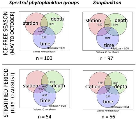
Variance partitioning of spectral phytoplankton groups and of zooplankton community structure by: station (A, B and C), depth (epilimnion and deep layer) and time (Day). The top row shows the results from across the ice-free season (top row), while the bottom row shows results restricted to time points in the stratification period of July and August only. The number of observations (n) is indicated below each plot.
Summary statistics for the dominant phytoplankton and zooplankton abundances depending on periods in surface and bottom.
| (a) | Surface | Bottom | ||||||||||||||||
|---|---|---|---|---|---|---|---|---|---|---|---|---|---|---|---|---|---|---|
| Period 1 | Period 2 | Period 3 | Period 4 | Period 1 | Period 2 | Period 3 | Period 4 | |||||||||||
| Species | Mean | ±stand. Dev. | Mean | ±stand. Dev. | Mean | ±stand. Dev. | Mean | ±stand. Dev. | Mean | ±stand. Dev. | Mean | ±stand. Dev. | Mean | ±stand. Dev. | Mean | ±stand. Dev. | ||
| Aphanizomenon flos-aquae | 10 | 17 | 300 | 540 | 41 | 60 | 21 | 21 | 0 | 0 | 9 | 13 | 89 | 197 | 3 | 5 | ||
| Aphanizomenon yezoense | 460 | 754 | 1865 | 1517 | 2707 | 1688 | 406 | 291 | 96 | 166 | 10879 | 8945 | 468 | 901 | 712 | 1033 | ||
| Aphanocapsa conferta | 7 | 12 | 195 | 306 | 298 | 222 | 2 | 4 | 0 | 0 | 194 | 198 | 41 | 52 | 2 | 4 | ||
| Aphanocapsa delicatissima | 262 | 454 | 1 968 | 2 001 | 64 | 105 | 0 | 0 | 0 | 0 | 21 612 | 38 365 | 682 | 1 102 | 618 | 892 | ||
| Aphanothece bachmannii | 37 | 51 | 264 | 353 | 26 068 | 21 662 | 27 239 | 31 893 | 2 186 | 3 511 | 26 372 | 24 381 | 39 905 | 22 664 | 12 411 | 13 039 | ||
| Aphanothece clathrata | 0 | 0 | 740 | 1 152 | 2 233 | 3 833 | 2 700 | 4 443 | 1 702 | 2 716 | 2 085 | 3 842 | 23 698 | 51 873 | 10 648 | 12 670 | ||
| Botryococcus braunii | 4 834 | 7 150 | 6 540 | 9 380 | 26 770 | 24 874 | 47 804 | 53 581 | 2 789 | 3 981 | 20 664 | 17 802 | 6 754 | 9 648 | 26 467 | 44 970 | ||
| Chroococcus sp. | 53 727 | 17 621 | 50 015 | 67 749 | 138 642 | 139 148 | 61 639 | 48 394 | 32 257 | 6 894 | 89 910 | 171 385 | 49 576 | 38 092 | 121 112 | 148 782 | ||
| Coelosphaerium kuetsingianum | 0 | 0 | 41 828 | 69 063 | 140 151 | 215 882 | 16 | 28 | 0 | 0 | 23 416 | 22 421 | 28 202 | 39 968 | 7 529 | 13 041 | ||
| Cyanodiction imperfectum | 0 | 0 | 384 | 777 | 360 | 785 | 0 | 0 | 0 | 0 | 681 | 1 022 | 210 | 469 | 0 | 0 | ||
| Desmerella brachycalyx | 57 | 46 | 52 | 79 | 207 | 239 | 142 | 142 | 16 | 24 | 53 | 78 | 297 | 102 | 422 | 438 | ||
| Dictyosphaerium pulchellum | 701 | 921 | 204 | 300 | 16 835 | 11 218 | 33 195 | 11 093 | 1 179 | 1 922 | 2 373 | 3 294 | 33 156 | 23 550 | 8 242 | 8 596 | ||
| Dolichospermum flos aquae | 0 | 0 | 3 438 | 4 924 | 14 826 | 33 153 | 159 103 | 154 345 | 0 | 0 | 320 | 715 | 0 | 0 | 67 258 | 99 224 | ||
| Dolichospermum solitaria var. planctonica | 51 | 60 | 43 | 75 | 203 | 213 | 0 | 0 | 96 | 96 | 127 | 240 | 116 | 97 | 163 | 65 | ||
| Dolichospermum spiroides | 6 | 11 | 7 | 16 | 0 | 0 | 13 | 22 | 0 | 0 | 10 | 22 | 0 | 0 | 0 | 0 | ||
| Limnothrix rosea | 2 | 3 | 0 | 0 | 0 | 0 | 11 | 19 | 46 | 63 | 2 | 5 | 3 693 | 5 500 | 0 | 0 | ||
| Merismopedia tenuissima | 0 | 0 | 0 | 0 | 34 | 76 | 0 | 0 | 0 | 0 | 0 | 0 | 864 | 1 484 | 195 | 218 | ||
| Microcystis wesenbergii | 22 | 38 | 460 | 789 | 341 | 329 | 342 | 560 | 540 | 935 | 343 | 324 | 12 051 | 26 948 | 17 561 | 23 797 | ||
| Planktolyngbya pseudospirulina | 172 | 187 | 69 | 79 | 4 754 | 4 872 | 3 112 | 2 304 | 5 397 | 7 201 | 8 829 | 9 274 | 51 624 | 30 500 | 3 297 | 2 457 | ||
| Planktothrix agardhii | 1 | 1 | 0 | 0 | 905 | 1 999 | 0 | 0 | 550 | 953 | 4 | 10 | 14 226 | 18 827 | 224 | 388 | ||
| Snowella septentrionalis | 0 | 0 | 0 | 0 | 0 | 0 | 256 | 443 | 0 | 0 | 0 | 0 | 1 007 | 2 251 | 3 557 | 4 346 | ||
| Woronichinia naegeliana | 0 | 0 | 124 | 165 | 676 | 591 | 5 716 | 2 245 | 23 | 39 | 298 | 291 | 682 | 320 | 823 | 724 | ||
| (b) | ||||||||||||||||||
| Period 1 | Period 2 | Period 3 | Period 4 | |||||||||||||||
| Mean | ±Stand. Dev. | Mean | ±Stand. Dev. | Mean | ±Stand. Dev. | Mean | ±Stand. Dev. | |||||||||||
| Diaphanosoma birgei | 22 | 13 | 1357 | 938 | 479 | 213 | 110 | 36 | ||||||||||
| Skistodiaptomus oregonensis | 698 | 699 | 819 | 459 | 720 | 415 | 634 | 145 | ||||||||||
| Daphnia dubia | 1384 | 1837 | 679 | 657 | 1758 | 754 | 3352 | 2305 | ||||||||||
| Eubosmina coregoni | 131 | 126 | 1 | 2 | 6 | 6 | 4 | 2 | ||||||||||
| Daphnia ambigua | 0 | 0 | 147 | 88 | 214 | 61 | 420 | 37 | ||||||||||
| Mesocyclops edax | 1021 | 1159 | 99 | 70 | 113 | 54 | 75 | 35 | ||||||||||
(a) Phytoplankton abundance in number of cells per mL and (b) Zooplankton abundances in number of individuals per 100 L
Four planktonic assemblage seasonal succession periods
To highlight successional (Table II) periods and covariation in planktonic assemblages, a co-inertia analysis on phytoplankton and zooplankton assemblages was performed (Fig. 3—see Fig. S6 for detailed plots), revealing four common periods: the spring period P1 (02/05/2007 to 10/07/2007 included) on the right of the plot, the early summer period P2 (24/07/2009 to 09/08/2007 included) at the top of the plot, the summer P3 (21/08/2007 to 07/09/2007 included) and the late summer period P4 (11/09/2007 to 11/10/2007 included). The shift from P1 to P2 (Fig. 3) corresponded to the strong summer increase in stratification (Fig. 1a), coupled with lower concentrations of dissolved phosphorus (DP) in the epilimnion (Fig. 1c) and a deep euphotic zone (ZE) reaching almost the bottom of the lake, as discussed above. The shift from P2 to P3 (Fig. 3) corresponded to a decrease in stratification intensity, so that P3 was thus intermediate in terms of stratification (Fig. 1a). The euphotic depth also eroded from 6 to 4.5 m. P4 (Fig. 3) marked the return of autumn conditions and the mixing of the depth layers in late September. P1 (Fig. 3) was dominated by chrysophyceae and diatoms (phytoplankton) and the copepod Mesocyclops edax (zooplankton). Cyanobacteria on the left side of the plot, dominated for the rest of the summer (P2 to P4). Filamentous phytoplankton species, such as Dolichospermum (Dolichospermum solitaria and Dolichospermum spiroides) and Aphanizomenon (Aphanizomenon flos-aquae and Aphanizomenon yezoense), were associated on the second axis with the zooplankton Diaphanosoma birgei (cladocera) and Skistodiaptomus oregonensis (copepod), in opposition to colonial phytoplankton species, such as Woronichinia naegeliana or Coelosphaerium and the cladoceran Daphnia dubia (Fig. 3). The second axis corresponded to a change in cyanobacterial succession, from Aphanizomenon and Dolichospermum (P2) to Planktothrix (P3) and finally Woronichinia (P4).
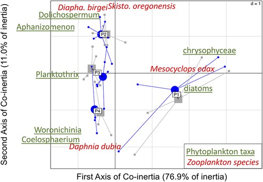
Sample plot of the co-inertia analysis performed on the PCA of the phytoplankton assemblage and the PCA performed on the zooplankton assemblage. The most dominant taxa are underlined for phytoplankton and in italic for zooplankton. Time periods (P1 to P4) are grouped by their barycenter, with periods seen from zooplankton (blue points) and from phytoplankton (gray squares). Detailed plots of co-inertia with all plankton taxa are shown in Fig. S4.
Seasonal dynamics of the DCM and surface assemblages
From mid-June to the seasonal overturn in mid-September, phytoplankton biomass was concentrated in a DCM near the lake bottom (Fig. S2). Initially dominated by the BROWNS spectral group (Chrysophyceae and diatoms), the DCM shifted to the BLUE-GREENs and MIXED spectral groups mid-July until the autumn overturn (Fig. S2). In June the diatoms Cyclotella (Cyclotella comta and Cyclotella glomerata) and the flagellate chrysophyceae Synura uvella dominated the DCM, while the epilimnetic assemblage was largely dominated by Cyclotella only (Fig. S3). In mid-July, the flagellate Cryptomonas erosa developed in the surface and the deep layers. For the rest of the summer, the DCM was dominated by phycocyanin-containing cyanobacteria, such as Aphanizomenon (A. flos-aquae and A. yezoense), Dolichospermum and Planktothrix agardhii (Fig. S3). The epilimnion was composed of small flagellates, such as Uroglena americana, Mallomonas (mainly Mallomonas bipunctuata, Mallomonas heterospina, Mallomonas pseudocoronata and Mallomonas tonsurata), Cryptomonas (mainly Cryptomonas borealis, C. erosa, Cryptomonas lucens, Cryptomonas marssoni and Cryptomonas ovata) and Trachelomonas (mainly Trachelomonas aculeata, Trachelomonas dybowskii, Trachelomonas intermedia, Trachelomonas hispida, Trachelomonas planctonica) until August (Fig. S3). Picocyanobacteria, such as Aphanothece (Aphanothece bachmannii and Aphanothece clathrata), were also observed in the epilimnion. At the end of August, the BLUE-GREENs spectral profile highlighted the presence of a double DCM, which persisted for two weeks (Fig. S2), with Aphanizomenon (A. flos-aquae and A. yezoense) in the uppermost layer and P. agardhii in the deeper layer (Fig. S4).
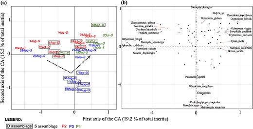
CA of the phytoplankton assemblages, from surface (S) and deep layer (D) during periods P2, P3 and P4. Plot (a) shows samples by date from the CA with B assemblages (names in framed) and S assemblages (names in italic). Periods are indicated by names in red, in blue and in green for P2, P3 and P4, respectively. In (b), the CA plot with species is shown (only the most contributing species are indicated). The black dotted arrow shows the divergence of B assemblage during P3.
To compare the species assemblages in the surface (S) and the deep layers (D) over time, a CA was performed on stratified periods P2, P3 and P4 (Fig. 4). P2 was distributed along the first axis, with surface phytoplankton (in red and italicized on Fig. 4) mixed on the plot with deep phytoplankton (in red and boxed on Fig. 4). During P3, the deep assemblage (in blue and boxed on Fig. 4) separated from surface assemblage (in blue and italicized in Fig. 4) along the second axis. During P4, both assemblages were grouped on the top right part of the plot (in green on Fig. 4). The deep and surface assemblages thus remained similar, except during P3, during which Planktolyngbya pseudospirulina, P. agardhii and Limnothrix rosea species increased in abundance at depth (Fig. 4). Based on non-parametric multivariate ANOVA, the surface assemblage significantly differed from the deep assemblage only during P3 (pseudo-F = 4.44; P = 0.026), but not during P2 and P4 (pseudo-F = 0.957; P = 0.45 and pseudo-F = 1.13; P = 0.41, respectively). Thus, differentiation did not occur during the strongest stratification period (P2), but only afterwards (P3). The seasonal overturn and a mixing of the assemblages occurred during P4.
Global diversity in the lake
Alpha (mean species richness) and gamma (total richness) were first calculated for each period and showed similar trends: a maximum diversity during P4 (seasonal overturn) and a minimum diversity during P3, although the differences between periods were not significant (Fig. 5a and b). When comparing beta diversity associated with the vertically distributed depth-layers, diversity increased with time, also being maximal during P4 (Fig. 5c).
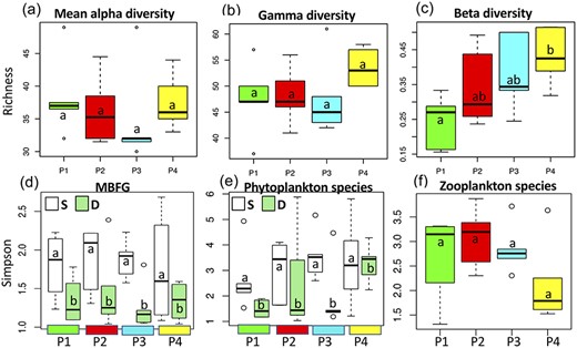
Boxplots of (a) mean alpha (|$\overline{\alpha}$|) and (b) gamma (|$\gamma$|) diversities, as well as (c) beta diversity (|$\beta =\gamma /\overline{\alpha}-1$|) by time period, for surface (S) and deep layer (D). Simpson diversity indices are calculated using (d) biomasses of the seven MBFG by period, (e) biomasses of phytoplankton species and (f) abundances of zooplankton species. Similar results are observed with Shannon and Eveness indices. Boxplots show the median, first and third quartiles, with minimum and maximum values at both ends. Boxes within each period that have different letters indicated are significantly different (P < 0.05).
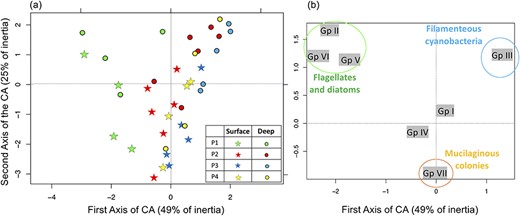
CA performed on the seven MBFG of phytoplankton (Kruk et al., 2010), with (a) plot of the samples and (b) plot of the MBFG.
Whether estimated as functional or taxonomic diversity, the surface assemblage (S) was always significantly more diverse than the deep assemblage (D) until P4 (Fig. 5d, e). In addition to cyanobacteria, several other functional groups contributed to the increasing functional diversity in the epilimnion (S), as observed in the CA of the seven MBFG (Fig. 6). The CA, which represents 74% of total inertia, distinguished groups II (small flagellates), V (medium and large flagellates) and VI (diatoms) from group III (filamentous cyanobacteria) on the first axis (Fig. 6b), with P1 and P3 situated at opposite extremes (Fig. 6a). The deep assemblage (D) was dominated by Aphanizomenon, Dolichospermum and P. agardhii, all from the same functional group (III), on the upper right quadrant of the CA (Fig. 6). Group VII (mucilaginous colonies including both cyanobacteria and chlorophyceae) increased in the bottom portion of the plot (Fig. 6b), as did most of surface assemblages (Fig. 6a). The first axis thus separated spring (P1) from the rest of the summer, while the second axis separated the assemblages according to depth. Flagellates and mucilaginous colonies thus contributed to increased functional diversity in the epilimnion compared with the deep layer. The seasonal overturn (P4) increased both species diversity and richness (Fig. 5a, b, e), without a corresponding increase in functional diversity (Fig. 5d). Zooplankton taxonomic diversity was at its lowest during the seasonal overturn (P4) (Fig. 5f).
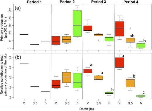
Boxplots of (a) GPP in the epilimnion (2 and 3.5 m depths) and the deep layer (5 m depth) and (b) relative contributions to the total production of the lake. Boxplots show the median, first and third quartiles, with minimum and maximum values at both ends. Sampling occurred on one date in P1, four dates in P2 and five dates in P3 and P4. Boxes within each period that have different letters indicated are significantly different (P < 0.05).
Contributions to primary production
Primary production was measured at three depths for one to five dates per period (Fig. 7). The upper layer was the most productive compared to the deeper one during P1, P3 and P4, while the DCM was the most productive during P2. When the relative contribution to total primary production was calculated based on depth stratum volume, we observed a similar pattern for P1, P3 and P4, with the upper layer contributing at least 50% of total production (Fig. 7). During P2, higher production in the DCM was compensated for by the larger water volume of the upper layer, so that the DCM contributed approximately 30% of the total production (Fig. 7). Despite a very low phytoplankton biomass in the epilimnion compared to the DCM, surface assemblage production contributed most during all summer owing to higher light availability associated with the larger epilimnetic volume. During P3, surface assemblage contributing much more (>90%) than the deeper layer to overall production (Fig. 7). Total production was the highest relative to the other periods during P3 across depths (Fig. S7).
Controlling factors of the DCM species
Cyanobacteria abundances were all positively explained by stratification intensity (PE) in the linear models (Table Ia). Abundance of the herbivorous zooplankton S. oregonensis was most related to variation in cyanobacteria, positively affecting epilimnetic species (A. yezoense and both Dolichospermum) and negatively affecting strictly deep-occurring species (P. agardhii). Several Aphanizomenon species were observed both in the epilimnion in early summer and in the DCM in late summer (Fig. S3). The abundance of A. flos-aquae was negatively affected by temperature and by the concentration of DN, with a positive interaction between DN and temperature (Table Ia). A. yezoense was positively influenced by PE and its variation (ΔPE indicating rapid warming or cooling), negatively by the concentration in DP, and with a positive interaction of effects of temperature and DP. Both Dolichospermum species were also observed in the epilimnion and in the DCM in July, with D. spiroides occurring earlier in season than D. solitaria. For D. solitaria, most of the environmental parameters were selected in the final model, but the coefficients were not significant, so the result was similar for D. spiroides. Abundances of both species were significantly and positively related to stratification (PE) and to abundances of the zooplankton S. oregonensis (Table Ia). P. agardhii occurred in the deep layer during P3, at the same time that DP and DN increased over the entire water column (Fig. 1c and d). Its abundance was positively related (in order of importance) to DN concentration, PE and to zooplankton abundances D. dubia and negatively related to S. oregonensis. Stratification was the main driver of cyanobacterial abundance and composition.
Macrozooplankton dynamics
The three dominant herbivorous zooplankton species were all explained by three parameters: water temperature, biomass of the ‘MIXED’ spectral group and abundance of the predatory copepod M. edax (Table Ib). Abundances increased with water temperature and with ‘MIXED’ biomass, corresponding to cryptophyta, as no phycoerythrin-containing cyanobacteria were observed in our microscopic analyses. Abundances of two cyanobacterial species were also positively related to the abundances of two zooplankton species: A. flos-aquae with D. birgei and P. agardhii with D. dubia. However, coefficients were very low, indicating a low contribution (Table Ib). D. dubia was also negatively correlated to potential energy PE (Table Ib) as it experienced increasing abundances in the fall when overturn was occurring (Fig.S4).
DISCUSSION
We addressed four main hypotheses in this detailed study of the vertical segregation of phytoplankton assemblages, the repercussions for the diversity and primary production, and the associated changes in zooplankton assemblages. In the study lake, which is moderately deep for its size, the vertical temperature and resource gradients were strong and constrained the phytoplankton assemblages. We hypothesized that vertical structuring in phytoplankton assemblages would be controlled by lake stratification and that strong density stratification should reduce entrainment of deeper water and the incorporation of metalimnetic species into the epilimnion (Serra et al., 2007). Different assemblages between the surface and the deep layers were expected, and predicted to result in increased beta diversity (along the vertical gradient) and in overall lake (gamma) diversity. We also expected the deep assemblage to contribute more to total primary production than the surface assemblage and that the zooplankton community would change in response to lake stratification and phytoplankton vertical structuring. We identified four periods of stratification intensity. Only one was associated with a vertical structuring of phytoplankton assemblages, without increase of either diversity or primary production. Instead, the period of maximal diversity corresponded to the seasonal transition. We first discuss the vertical structuring of phytoplankton assemblages in relation to stratification and resource gradients, followed by a discussion of the diversity and primary production responses.
We observed that surface and deep assemblages were similar during the strongest stratification period (P2), and then diverged into two distinct assemblages during P3, despite decreased stratification. Similar assemblages during strong stratification could result when the DCM represents an accumulation of surface-settling species (Cullen, 1982; Condie and Bormans, 1997) and/or when a portion of species in the DCM become entrained by internal waves and deep water upwelling (Bormans et al., 2004). Both contributions were observed in our study, during P1 and P2 respectively. Indeed, until mid-July (P1), phytoplankton biomass was dominated by diatoms (especially C. comta and C. glomerate) in the epilimnion and in the deep layer. These small centric diatoms, would have been subject to sedimentation loss and accumulation in deeper waters (Fahnenstiel and Glime, 1983; Jackson et al., 1990). Motile chrysophyta, with the spring species S. uvella and Dinobryon divergens, also accumulated in the deep layer. S. uvella is also typical of small oligotrophic lakes and heterotrophic ponds, and may have accumulated at the bottom of the lake because of higher CO2 levels (Reynolds, 2006) These species are also known to be mixotrophs (Reynolds, 2006) and able to benefit from likely higher bacterial populations at depth.
During P2, we observed the second period of similar deep and surface phytoplankton assemblages, in this case resulting from entrainment of deeper assemblages towards the surface. Recurrent internal waves associated with daily wind have been demonstrated in the study lake during the summer months (Pannard et al., 2011). The DCM composition shifted to cyanobacteria at the end of July and for the rest of the summer, with dominance by Aphanizomenon (A. flos-aquae and A. yezoense) and Dolichospermum (D. solitaria and D. spiroides). Aphanizomenon and Dolichospermum are representative of the functional group H1, in Reynolds’ classification and are sensitive to poor light and low phosphorus concentrations (Reynolds et al., 2002). Epilimnetic phosphorus concentrations remained low and consequently potentially limiting for growth at <0.13 μmol P L−1; most half-saturation constants for phosphorus uptake being above 0.16 μmol P L−1 (Reynolds, 2006; Edwards et al., 2012; Bestion et al., 2018). Aphanizomenon and Dolichospermum were able to develop large biomasses in the DCM, most likely due to the upward input of P and N from the anoxic sediment, possible as long as the euphotic zone reached the bottom of the lake. The contribution of internal loading compared with external loading has been already highlighted in our study lake (Planas and Paquet, 2016). A portion of the DCM species would have been entrained into the epilimnion during P2 owing to shear stress associated with the occurrence of internal waves (Pannard et al., 2011). Anecdotally, we noted that cyanobacterial aggregates likely originating in the DCM were regularly observed floating at the lake’s surface, disappearing a few days later as apparently low surface phosphorus concentrations precluded the growth of cyanobacteria in the epilimnion.
During P2, the DCM was thus a source of species for the surface layer phytoplankton assemblage and in particular, the filamentous cyanobacteria. However, small flagellated species, specific to the epilimnion continued to be observed, albeit at low abundances: Cryptomonas (C. marssonii, C. erosa), U. americana, Trachelomonas (T. intermedia, T. dybowskii, T. aculeate), Scourfieldia cordiformis, Erkenia subaequiciliata, Ochromonas globosa, Mallomonas acaroides, and Chlamydomonas (C. fusus, C. dinobryonii). With a high surface: volume ratio, small species are known to tolerate low nutrient concentrations and their ability to perform flagellar movement reduces sinking loss (Reynolds, 2006). Their small cell size, buoyancy regulation and motility associated with flagella are all functional traits related to preventing sinking loss (Salmaso et al., 2015). These species may have contributed to primary production in the surface layer, keeping relative surface production higher than deep water production as observed. Such species would likely also have benefitted the zooplankton assemblage: we observed a positive correlation between the biomass of the ‘MIXED’ spectral group and the abundances of the three herbivorous zooplankton. Finally, during the period of strong stratification (P2), surface nutrient limitation favored the occurrence of oligotrophic surface species above deep filamentous cyanobacteria, the latter likely fueled by vertical nutrient fluxes from the anoxic sediments. However, it should be noted that the two phytoplankton assemblages were not significantly distinguishable statistically. Thus, stratification intensity may not have been sufficient to impede the vertical movement of DCM species (Abbott et al., 1984) and the shear stress associated with internal waves may have further inhibited spatial segregation.
By mid-August, thermal stratification had decreased, following rainfall and wind events, thereby reducing vertical gradients of nutrients and light (P3). At this point in time, the two assemblages differed significantly with the development of shade-adapted species in the deep layer and the continued presence of the epilimnetic species from the P2 phase at the surface. Some picocyanobacteria (A. clathrata, A. bachmannii, Aphanocapsa delicatissima, A. conferta) were also observed in the epilimnion. Metalimnetic species are well described in the literature, in particular with respect to their chromatic adaptation to low light conditions and buoyancy regulation capacities (Dokulil and Teubner, 2000; Walsby, 2005). Here we observed P. agardhii, P. pseudospirulina and Limnothrix (L. rosea and L. redekei), which are known to tolerate highly light-deficient conditions and are all known to be metalimnetic in distribution (Reynolds, 2006). Planktothrix rubescens, a phycoerythrin species (the red Planktothrix), is known to accumulate in the metalimnion of deep lakes (Walsby and Schanz, 2002; Oberhaus et al., 2007) where light is composed primarily of green wavelengths, thus forcing the species to use phycoerythrin or another red pigment (Stomp, 2008). In our study lake, the DCM was located at a depth of only five meters enabling dominance instead of the ‘green Planktothrix’ (P. agardhii); this ‘green’ species more commonly in turbid well-mixed waters (Mantzouki et al., 2016) where it can accumulate in DCMs (Utkilen et al., 1985; Reichwaldt and Abrusan, 2007) at similar depths as the ‘red’ species (Halstvedt et al., 2007). At the end of P3, two distinct layers were observed within the DCM, with a peak of Aphanizomenon above a Planktothrix peak. Such a spatial segregation, with two peaks of Aphanizomenon above P. rubescens, has already been observed in a deep lake (69 m) and attributed to a spatial niche segregation of light and nutrients (Selmeczy et al., 2016). The seasonal overturn during P4 ended this vertical structuring of assemblages.
We expected species richness to increase with vertical structuring of phytoplankton assemblages, associated with the vertical resource gradient. The exploitation of the resource gradients through the use of motility traits (flagella versus gas vacuoles) can reduce spatial overlap between species, and sometimes lead to greater taxonomic and functional diversities (Beisner and Longhi, 2013; Ouellet Jobin and Beisner, 2014). Instead, in our study, species richness did not increase with vertical structuring of phytoplankton assemblages, but rather decreased during P3. During this time light availability decreased in the deepest layer, resulting in more selective environmental conditions and thus reduced diversity. Only shade-adapted species, such as Planktothrix, Planktolyngbya and Limnothrix, were able to develop in deep layer during P3. Small, motile species adapted to oligotrophic conditions increased surface taxonomic and functional diversities, from P1 to P3. When focusing on functional diversity calculated with the seven MBFG (Kruk et al. 2010) instead of the two hundred species of the entire community, the summer epilimnetic assemblages (P1, P2 and P3) were thus the most diverse with the presence of almost all groups, while the deep layer was dominated by filamentous cyanobacteria. The seasonal overturn (P4) mixed the surface and deep assemblages and was demonstrated to be the most diverse period for phytoplankton assemblages in taxonomic diversity, but without a corresponding increase in functional diversity. The erosion of thermal stratification led to epilimnetic increases in phosphorus availability and favored the return of fall species, such as W. naegeliana. This seasonal disturbance enabled the highest alpha, beta and gamma diversities, favoring coexistence of late summer and fall species.
We also expected the DCM to contribute significantly to the overall lake production, especially in a relatively shallow and small lake. The vertical distribution of phytoplankton biomass was typical of a clear vertically stratified oligotrophic lake (Fee, 1976; Cullen, 1982), with a DCM. During summer (P1 to P3), epilimnetic biomass remained very low (<12 μg chla L−1) in contrast to the deep layer biomass (>200 μg chla L−1). It appears that the clear epilimnion allowed light to reach the deep layer. The control of DCM by stratification and light is already well described (Abbott et al., 1984; Leach et al., 2018), with vertical gradient in nutrients and light explaining DCM dynamics (Fee, 1976; Klausmeier and Litchman, 2001). During the most strongly stratified period, one could have expected a larger production by the DCM compared with the clear epilimnion, even when production is weighted by the volume of the two layers (based on data from a bathymetric map performed the same year). Because the area of the epilimnetic layer was larger, the volume of this layer is much bigger than that of the deep layer and this compensated for the concentrated deep layer production. Despite high deep layer primary production during P2, surface production integrated over the epilimnion was systematically higher. This epilimnetic production could have fueled zooplankton assemblage production, favoring competitive species able to grow at low resource concentrations and on small flagellates. The relative contribution to total production of the shade-adapted DCM species was even lower during P3 (<10%) than during P2, and could be considered negligible for lake primary production. There the occurrence of a DCM with a distinct phytoplankton assemblage did not lead to increases in diversity and its contribution to overall primary production remained limited.
Four periods were highlighted in the plankton assemblage compositions, differing mainly according to stratification intensity and surface DP availability. Ice cover on the study lake thawed in early May, but with rapid heating was already stratified by mid-May. It remained thermally stratified throughout the summer, with recurrent internal waves occurring every day (Pannard et al., 2011). Other than the fall species, W. naegeliana, the abundances of cyanobacteria were all explained by stratification intensity, measured as potential energy. Stratification is known to be a critical driver of cyanobacteria blooms, either directly or through stratification-induced internal nutrient loading (Huber et al., 2012). The four phytoplankton-determined periods were also reflected in the zooplankton assemblages. M. edax characterized P1 (spring), with diatoms and chrysophyceae. D. birgei characterized P2 with Dolichospermum and Aphanizomenon during high stratification. D. dubia showed the greatest biomass during P4 (overturn), co-occurring with mucilaginous phytoplankton species. Phytoplankton-zooplankton covariations were the result of common control factors, such as stratification and temperature, and of trophic interactions. Here, all the herbivorous species were explained by temperature, the abundance of the predator M. edax and the biomass of cryptophyceae prey. Temperature can have a direct effect on zooplankton growth (Shuter and Ing, 1997), and an indirect effect via stratification (Thackeray et al., 2006). Disentangling the effects of biotic and abiotic factors and prioritizing them are not possible in observational field studies such as ours without further experimental manipulation. Experiments have shown that warmer temperatures accelerate Daphnia grazing and growth, but not growth of phytoplankton which are more controlled by depth stratification, through light availability (Berger et al., 2006). We observed that the cryptophyceae occurred at greater biomass in the epilimnion than in the deep layer. Zooplankton, such as Diaphanosoma may feed selectively on cryptophyceae and it has been demonstrated that grazing rates by small zooplankton especially, is not reduced in presence of filamentous cyanobacteria (Kirk and Gilbert, 1992). Daphnia are also able to consume short filaments of Planktothrix (Reynolds, 2006) and in line with this, we observed that Daphnia abundances were correlated to Planktothrix by the linear models (although with a very small coefficient).
The major aim of this study was to determine whether the vertical resource gradient in a small oligotrophic lake could lead to a spatial segregation of phytoplankton assemblages with benefits for overall depth-integrated diversity and production. The small size of the lake studied allowed us to ignore horizontal heterogeneity and horizontal advection. Our lake displayed a DCM, a common feature of deeper oligotrophic lakes and implying a vertical segregation of phytoplankton biomass, but our study demonstrated no benefit at the scale of the lake of the presence of this DCM for primary production and diversity, whether functional or taxonomic. Instead, phytoplankton diversity was favored by mixing during the seasonal transition associated with succession. This suggests that a shallower lake depth might negatively affect spatial segregation, although a previous multi-lake snapshot survey suggested that vertical spatial overlap of phytoplankton spectral groups is rather controlled by stratification, the optical depth (size of the light niche) and the lake trophy (Beisner and Longhi, 2013). Compared to deeply stratified lake, the depth over which spatial segregation of phytoplankton could occur in our shallow lake is reduced, potentially increasing the overlap in competing spectral groups, with negative consequences for diversity (Ouellet Jobin and Beisner, 2014). Stratification, which is controlled by climatic forcing, is the prerequisite for DCM establishment. Light availability is also directly controlled by climate, as well as vertical nutrient fluxes which depend on wind forcing (MacIntyre et al., 2006). It is thus expected that the dynamics of DCM will change from year to year. However, the properties of the DCM can be well predicted from the euphotic depth and DOC concentration for DCM depth, and from lake size and maximum depth for DCM thickness (Leach et al., 2018). These parameters are quite stable between years, with some exceptions. An increase in turbidity due to glacial clay or volcanic ashes for instance makes DCMs shallower (Modenutti et al., 2013). In another exception, a DCM does not occur each summer in Lake Erie despite strong stratification; depending on meteorological forcing and resuspension events (Bramburger and Reavie, 2016; Lick et al., 1994). Finally, light seems to be the main driver of DCM properties (biomass and depth), more so than stratification or phosphorus in southern lakes from Antarctica to the tropics (Burnett et al., 2006; Leach et al., 2018; Sanful et al., 2019).
CONCLUSION
In this study, we demonstrated a low contribution of the DCM to lake phytoplankton diversity and primary production, in a small but relatively deep lake (maximum depth of 7.2 m). The DCM production represented on average 33% of total production during the strongest summer stratification period, during which surface and deep assemblages were the same. When surface and deep assemblages diverged, the taxonomic and functional diversity at the scale of the water column decreased. The distinct surface and deep phytoplankton assemblages were within 3 m of each other. Such lakes with intermediate depth represent good opportunity to study strong vertical clines over a small scale, which may allow both the niche partitioning but also facilitate the mobile species migration among habitats.
Acknowledgements
We thank S. Paquet, C. Beauchemin, P. Marcoux, and K. McMeekin for field and laboratory assistance and for the bathymetry of the lake (S. Paquet). We thank the Action de conservation du bassin versant du lac Bromont for the infrastructure support, and for logistical help in the field and the municipality for the bathymetric map. We thank the Interuniversity Limnology Research Group/Groupe de recherche interuniversitaire en limnogie (GRIL) for providing funding to AP to spend time in 2019 as an invited professor at UQAM to analyze the data from the field survey performed in 2007. We thank John Dolan and two anonymous referees for helpful comments on an earlier version of the manuscript. The authors declare that they have no conflict of interest.
FUNDING
This work was supported by a grant from the Fonds Québécois de la Recherche sur la Nature et les Technologies to David F. Bird, B.E.B., and D.P. and by the Groupe de Recherche Interuniversitaire en Limnologie.
AUTHORS’ CONTRIBUTIONS
A.P., D.P. and B.E.B. designed the study. A.P. and M.J. collected the data. A.P. assembled and analyzed the data. P.LN. performed the linear models. A.P., B.E.B., D.P., P.LN and M.B. wrote the manuscript.
References
Abbott, M. R., Denman, K. L., Powell, T. M., Richerson, P. J., Richards, R. C., and Goldman, C. R. (
Anneville, O., Gammeter, S., and Straile, D. (
Bestion, E., Schaum, C. E., and Yvon-Durocher, G. (
Bormans, M., Ford, P. W., Fabbro, L., and Hancock, G. (
Burnett, L., Moorhead, D., Hawes, I., and Howard-Williams, C. (
Carignan, R., Blais, A. M., and Vis, C. (
Edwards, K. F., Thomas, M. K., Klausmeier, C. A., and Litchman, E. (
Halstvedt, C. B., Rohrlack, T., Andersen, T., Skulberg, O., and Edvardsen, B. (
Heino, J., Grönroos, M., Ilmonen, J., Karhu, T., Niva, M., and Paasivirta, L. (
Hillebrand, H., Dürselen, C. D., Kirschtel, D., Pollingher, U., and Zohary, T. (
Jackson, L. J., Stockner, J. G., and Harrison, P. J. (
Jacquet, S., Briand, J. F., Leboulanger, C., Avois-Jacquet, C., Oberhaus, L., Tassin, B., Vinçon-Leite, B., Paolini, G. et al. (
Kruk, C., Huszar, V. L., Peeters, E. T., Bonilla, S., Costa, L., Lürling, M., Reynolds, C. S. et al. (
Korhonen, J. J., Wang, J., and Soininen, J. (
Leach, T. H., Beisner, B. E., Carey, C. C., Pernica, P., Rose, K. C., Huot, Brentrup, J. A., Domaizon, I. (
Lick, W., Lick, J., and Ziegler, C. K. (
Lund, J. W. G., Kipling, C., and Le Cren, E. D. (
MacIntyre, S., Sickman, J. O., Goldthwait, S. A., and Kling, G. W. (
Mantzouki, E., Visser, P. M., Bormans, M., and Ibelings, B. W. (
Massicotte, P., Frenette, J. J., Proulx, R., Pinel-Alloul, B., and Bertolo, A. (
Modenutti, B., Balseiro, E., Navarro, M. B., Laspoumaderes, C., Souza, M. S., and Cuassolo, F. (
Oberhaus, L., Briand, J. F., Leboulanger, C., Jacquet, S., and Humbert, J. F. (
Padisák, J., Barbosa, F. A. R., Koschel, R., and Krienitz, L. (
Palmer, M. A., Menninger, H. L., and Bernhardt, E. (
Pannard, A., Beisner, B. E., Bird, D. F., Braun, J., Planas, D., and Bormans, M. (
Pigot, A. L., Trisos, C. H., and Tobias, J. A. (
Pinel-Alloul, B., Ghadouani, A., and Gélinas, M. (
Pomati, F., Matthews, B., Jokela, J., Schildknecht, A., and Ibelings, B. W. (
Read, Q. D., Baiser, B., Grady, J. M., Zarnetske, P. L., Record, S., and Belmaker, J. (
Reynolds, C. S., Huszar, V., Kruk, C., Naselli-Flores, L., and Melo, S. (
Salmaso, N., Naselli-Flores, L., and Padisak, J. (
Sanful, P. O., Otu, M. K., Kling, H. W., and Hecky, R. E. (
Saros, J. E., Interlandi, S. J., Doyle, S., Michel, T. J., and Williamson, C. E. (
Selmeczy, G. B., Tapolczai, K., Casper, P., Krienitz, L., and Padisák, J. (
Serra, T., Vidal, J., Casamitjana, X., Soler, M., and Colomer, J. (
Simpson, J., Edelsten, D., Edwards, A. and Morris, N. (
Tamme, R., Hiiesalu, I., Laanisto, L., Szava-Kovats, R., and Pärtel, M. (
Tews, J., Brose, U., Grimm, V., Tielbörger, K., Wichmann, M. C., Schwager, M., and Jeltsch, F. (
Thackeray, S. J., George, D. G., Jones, R. I., and Winfield, I. J. (
White, E. P., Ernest, S. M., Adler, P. B., Hurlbert, A. H., and Lyons, S. K. (
Author notes
present address: cnrs-umr 6553 ecobio, osur, university of rennes 1, campus de beaulieu, bâtiment 14b, av. general leclerc, rennes f-35 042, france
