


Abstract
Body size is an important functional trait that can be indicative of ecosystem structure and constraints on growth. Both increasing temperatures and eutrophication of lakes have been associated with a shift toward smaller zooplankton taxa. This is important in the context of climate change, as most aquatic habitats are expected to warm over the coming decades. Our study uses data from over 1000 lakes surveyed across a range of latitudes (26–49°N) and surface temperatures (10–35°C) in the USA during the spring/summer of 2012 to characterize pelagic cladoceran body size distributions. We used univariate and multiple regression modeling to determine which environmental parameters were strongly correlated to cladoceran body size. A strong positive correlation was observed between cladoceran body size and latitude, while a strong negative correlation was observed between cladoceran body size and water temperature. The ratio of zooplankton to phytoplankton, as well as relative total biomass contributions by cladocerans, decreased as trophic state increased. Multiple regression identified temperature-related variables and water clarity as significantly affecting cladoceran body size. These observations demonstrate the dual threat of climate change and eutrophication on lake ecosystems and highlight potential changes in biogeographical patterns of zooplankton as lakes warm.
INTRODUCTION
Lake ecosystems face multiple stressors as climates warm. These can include cycles of extreme drought and floods (Wantzen et al., 2008), prolonged and intensified thermal stratification (Kraemer et al., 2015) and shifts in aquatic community composition and phenology (Winder and Schindler, 2004; Thackeray et al., 2008). In addition to the challenges faced by warming, many lakes are also undergoing eutrophication due to agricultural and industrial development of watersheds (Carpenter et al., 1998; Qin et al., 2013). Eutrophication in lake ecosystems has been associated with shifts from macrophyte-dominated clear water to phytoplankton-dominated turbid water (Jeppesen et al., 2000; Qin et al., 2013), intensified hypoxia leading to fish-kills (Müller and Stadelmann, 2004) and changes in zooplankton community structure (Straile and Geller, 1998; Jeppesen et al., 2000). Climate warming and eutrophication represent concurrent threats to lake ecosystems worldwide and the effects of these two forces may enhance one another (Jeppesen et al., 2010). For example, climate warming can accelerate eutrophication by intensification of storm events that promote excess nutrient runoff from terrestrial sources, while eutrophication may in turn exacerbate the effects of climate change via release of methane from deoxygenated waters (Moss et al., 2011).
Ecological theory predicts smaller body size at warmer temperatures. Bergmann’s rule (Bergmann, 1847) states that within a broadly distributed taxonomic clade, larger species within the clade will be more prevalent toward the poles, while smaller species within the clade will be dominant in warmer regions. This principle has been observed in several field studies of both endotherms and ectotherms (Millien et al., 2006), although temperature may be an indirect factor in constricting these distributions (Angilletta and Dunham, 2003). One explanation for this pattern in endotherms is that increased body size enhances an organism’s ability to conserve heat. For ectotherms, the observed “temperature-size rule” (Atkinson, 1994) may have more to do with ontogenetic effects of rearing temperatures, with those organisms reared at higher temperatures exhibiting smaller body size. Growth rate of individuals may be dependent on available resources and an organism’s innate abilities to allocate energy toward capitalizing on those resources (Kozłowski et al. 2004). For aquatic organisms, reduction of oxygen at warmer temperatures may also constrain body size (Atkinson, 1994). It logically follows that a projected consequence of climate warming in many ecosystems is a decrease in average body size on a community level (Daufresne et al., 2009; Sheridan and Bickford, 2011). This may be due to a shift in species range distributions toward higher latitudes or elevations for taxa with narrow temperature constraints (Walther et al., 2002; Chen et al., 2011), or to phenotypical adaptation within a population over successive generations (Schmidt and Jensen, 2003). This effect may also be a consequence of shifting ecological structure stemming from climatic changes (Brown et al., 1997; Stenseth et al., 2002; Manca and DeMott, 2009).
The temperature-size rule was observed for pelagic cladoceran zooplankton in a seminal study by Gillooly and Dodson (2000), which found that increasing cladoceran body size (using measurements gleaned from literature and taxonomic keys) was strongly correlated to increasing latitude. These results were supported by a later study of cladocerans in lakes ranging from the arctic to the equator (Havens et al., 2015a), and by a recent study (Rizo et al., 2019) which found that body size of cladocerans was reduced on average in tropical regions when compared with temperate regions. In the case of cladocerans, this pattern may be a result of thermal constraints on particular taxa, specifically Daphnia spp. (Gillooly and Dodson, 2000), or increased predation pressure from planktivorous fish at lower latitudes (Brooks and Dodson, 1965; Dumont, 1994). Climate warming is projected to create increased fish habitat in lakes (De Stasio et al., 1996), which may affect the size structure of zooplankton communities. Several studies have shown decreasing zooplankton size with increasing water temperatures on both an individual (Moore and Folt, 1993; Daufresne et al., 2009) and community level (Šorf et al., 2015). Increasing eutrophication has also been associated with decreases in mean body size of zooplankton communities (Pace, 1986). Reduction in mean body size along an increasing trophic gradient has been attributed to a reduction in food quality (i.e. increases in large, inedible cyanobacterial colonies and filaments) (Ghadouani et al. 2006) and a shift from larger to smaller zooplankton species (Bays and Crisman, 1983; Canfield and Jones, 1996) likely due to increased predation pressure from planktivorous fishes in more productive systems. Mesocosm experiments that included both nutrient inputs and temperature increases (Šorf et al., 2015) found that cladoceran body size decreased with increasing temperature only when nutrients were high, suggesting that cladoceran communities in productive systems may be more sensitive to temperature increases as the climate warms.
Zooplankton serve as a critical ecological link between primary producers and higher-order consumers (fish, birds and mammals) in aquatic ecosystems. Body size is a functional trait that is closely related to evolutionary fitness (Brown et al., 2004; Hart and Bychek, 2011). Given the importance of zooplankton community size structure in relation to overall ecological function, there is a pressing need to examine the impacts of both increasing temperatures and eutrophication—arguably the two most imminent threats to lake water quality—on this important trait. Using lake and reservoir survey data from a broad geographic region encompassing multiple biomes and ecoregions (the conterminous USA), we assessed the relationship between pelagic cladoceran body size and temperature, as well as the relationship between pelagic cladoceran body size and lake trophic status. We followed, as closely as possible, the methods employed by Gillooly and Dodson (2000) in an attempt to confirm their findings using a single, large dataset with consistent methods and directly measured body lengths (as opposed to body lengths assumed from general reference texts, as was done for many species in that study). We hypothesized that cladoceran body size and lake surface temperatures would reflect patterns discovered by Gillooly and Dodson (2000), and that mean cladoceran body size would be positively correlated to increasing latitude and decreasing water temperatures. Since eutrophication is typically a result of local environmental factors and is not uniformly related to latitudinal or temperature gradients in the USA (Hollister et al., 2016), we further hypothesized that cladoceran body size would be reduced in productive systems regardless of geographic distribution of lakes. Our objective was to generate baseline data using near-current geographic patterns of cladoceran body sizes, which can be compared against data in future studies of cladoceran body size and zooplankton community structure as both eutrophication and climate change proceed in this region of the globe.
MATERIALS AND METHODS
Site selection
All data used in this study were collected during the US Environmental Protection Agency’s 2012 National Lakes Assessment (NLA). A total of 1038 lakes and reservoirs (hereinafter, lakes) within the conterminous USA were selected using a non-biased probability-based design to ensure even spatial distribution of lakes across major US ecoregions and between surface-area classes (USEPA, 2012a). Out of those 1038 lakes, a set of 91 reference lakes were hand-picked based on condition assessments from the 2007 NLA, in order to ensure that some lakes within the dataset were minimally disturbed. All lakes sampled during the 2012 NLA were at least 1 hectare in surface area and at least 1 m deep, with at least 0.1 hectares of open water area. Brackish and ephemeral lakes, as well as treatment/disposal ponds, were excluded from the survey, as were the five Laurentian Great Lakes and the Great Salt Lake. Each selected lake was sampled once in spring/summer (May through September) of 2012, except for a subset of lakes (n = 96 lakes) that were randomly selected for a second sampling event within the timeframe of the survey. Watershed land-use characteristics were obtained for each lake included in this study using methods described in Beaver et al. (2014) and Simley and Carswell (2009).
Zooplankton sampling and processing
Zooplankton tows were performed at an index site in each lake, representing the deepest point up to 50 m in natural lakes and the approximate midpoint in reservoirs. Five-meter vertical tows were performed during the daytime, using 150 μm mesh Wisconsin-style nets. For lakes shallower than 5 m, cumulative tows totaling 5 m depth were performed and all collected material was composited. Tow material was preserved in 70% ethanol upon collection. Zooplankton samples were then shipped to BSA Environmental Services, Inc. (Beachwood, OH, USA) for identification and enumeration. Samples were homogenized using a magnetic spinner at low speed and an appropriate subaliquot was drawn. Subaliquots were deposited in Utermöhl chambers and counted using inverted light microscopes (Wilovert) at magnifications up to ×400. Organisms were identified to lowest possible taxonomic level (usually species) by a team of trained taxonomists and enumerated to a tally of 400 total individuals. Nauplii, ostracods and rotifers were excluded from enumeration in samples collected with 150 μm nets and were instead enumerated in separate samples collected with a smaller mesh size. However, these smaller organisms (<20 μm), as well as copepodites, were excluded from our analyses. Up to 20 individual specimen measurements were taken for dominant species (>40 organisms observed), while up to 10 individual specimen measurements were taken for organisms observed 20–40 times in a subsample. Up to five individual measurements were taken for organisms encountered <20 times in a subsample. Mean lengths for each taxon were then computed for each sample and those means were used to estimate individual species biomass (McCauley, 1984). For lakes that were sampled twice within the survey, an average was computed for mean lengths between the two samples such that individual lakes remained the primary unit for comparison. For copepods, measurements were taken from the anterior tip of an individual specimen to the end of the caudal ramus (not including the caudal setae) and for cladocerans, measurements were taken from the anterior tip of the head to the base of the tail spine (Lawrence et al., 1987). Further details on laboratory procedures can be found in USEPA (USEPA, 2012b). All zooplankton biovolume and abundance data are publicly available from https://www.epa.gov/national-aquatic-resource-surveys/data-national-aquatic-resource-surveys.
In this study, only pelagic cladocerans were included in analyses. Excluded taxa were based on Gillooly and Dodson (2000) as follows: all Chydoridae except for C. sphaericus were excluded; all Sididae except Diaphanosoma spp. were excluded; all Macrothricidae, Simocephalus spp., Polyphemus spp. and Moina spp. were excluded. Samples collected from the state of Wisconsin (n = 128 lakes) were excluded due to inconsistencies in taxonomic methods. Mean body size for cladocerans and Daphnia spp. alone were plotted onto a map using ArcGIS.
Environmental variables
Surface water temperatures were computed as the mean temperature within the top 1 m of the water column at the index site. Chlorophyll-a and nutrient samples were collected from the index site. An integrated sampler (Minnesota Pollution Control Agency, USEPA 2012b, fig. 5.2) was used to fill a 4 L cubitainer. A 250 mL subsample for nutrient analysis was acidified and shipped overnight to processing labs. For chlorophyll-a, a subsample of up to 250 mL of water was pumped through a glass fiber filter using <7 inches of Hg pressure. Filters were then shaded from light and frozen until processing. Chlorophyll-a was determined fluorometrically following 90% acetone extraction within 30 days of sample collection. Total nitrogen and total phosphorus concentrations were determined using automated colorimetric analysis following persulfate digestion. Secchi depth was recorded using a standard Secchi disk on the shady side of the boat. When the Secchi disk was visible at the bottom, Secchi depth was assumed to be the index site depth. Further details on sampling procedures can be found in the NLA Laboratory Methods Manual (USEPA, 2012a).
Trophic state index (TSI) was determined using measured chlorophyll-a values with the equation provided in Carlson (1977). TSI can be determined using either chlorophyll-a, total phosphorus or Secchi depth. For this study chlorophyll-a was determined to match the contextual definition of trophic state most closely, which is the degree of biological production. Although all lakes fall somewhere on a continuous gradient of multiple trophic state variables rather than into distinct categories (Carlson and Simpson, 1996), for the purpose of this study lakes were organized into four TSI tiers as follows: oligotrophic if TSI ranged between 0 and 40; mesotrophic if TSI ranged between 40 and 50; eutrophic if TSI ranged between 50 and 70; hypereutrophic if TSI ranged between 70 and 100. Distributions of TSI were determined to be non-Gaussian (Shapiro–Wilk test). Kruskal–Wallis tests, followed by post hoc testing (Dunn’s test) were performed to determine differences in mean cladoceran body length and Daphnia spp. body length by TSI category. Percentage land use was also compared across TSI categories using Kruskal–Wallis tests followed by Dunn’s test. For comparison, univariate regression was performed between all cladoceran lengths and individual TSI values (see Supplementary Information).
Body length vs. latitude and temperature
To evaluate the hypothesis proposed by Gillooly and Dodson (2000) that cladoceran length is inversely proportional to latitude and water temperature, we fit univariate models describing the relationship of cladoceran body length with both temperature and latitude separately. Linear regressions (here and throughout the study) were performed in the R statistical language R Core Team (2020) using the car package (Fox and Weisberg, 2019) for model diagnostics.
For consistency with Gillooly and Dodson (2000), and because of the confounding effects that elevation has on water temperature as a function of latitude, we removed samples above 1000 m in elevation for regressions between body length and latitude and between body length and temperature. Samples were then binned into 1° N latitudinal intervals and mean surface water temperatures (0–1 m, °C) were calculated for each interval. Mean cladoceran body lengths were also calculated within each 1° N latitudinal interval (n = 23 intervals). Although the study by Gillooly and Dodson (2000) examined mean cladoceran length in 2.5° latitudinal intervals, we chose to use more restricted intervals since our study was much narrower in latitudinal range and included samples from the northern hemisphere only.
Zooplankton: phytoplankton ratio and community composition
The ratio of C-zooplankton:C-phytoplankton (ZC:PC, the ratio of estimated carbon content of crustacean zooplankton to the estimated carbon content of phytoplankton) was computed for all samples and mean ZC:PC was computed per 1°C surface temperature interval. Zooplankton carbon was estimated at one-half of crustacean (copepod and cladoceran) biomass (Latja and Salonen, 1978). Total phytoplankton carbon was calculated based on total biovolume estimates using the formula described in Rocha and Duncan (1985). To determine the relationship between ZC:PC and water temperature, linear regression was performed using mean ZC:PC per 1°C temperature interval (n = 19 intervals) as well as using all sampling events at elevations below 1000 m (n = 888). ZC:PC values were log10-transformed prior to regression against surface temperature (Yuan and Pollard, 2018). Lakes that fell within temperature intervals that had fewer than three samples within a 1°C range were excluded (all lakes with temperatures below 14°C and above 33°C). To determine spatial gradients in ZC:PC, we performed linear regression between latitude and ZC:PC using 1°N latitude intervals for all samples below 1000 m elevation (n = 888). Means of ZC:PC per 1°N latitude interval were log10-transformed prior to regression in order to achieve a normal distribution of samples. ZC:PC distributions were determined to be non-Gaussian and were compared across the four TSI categories using a Kruskal–Wallis test followed by Dunn’s test.
To investigate differences in community composition along both temperature and trophic gradients, relative percentages of total crustacean biomass for Daphnia spp., total Cladocera and total Copepoda (Cyclopoida and Calanoida) were computed for each sampling event. These data were then transformed into binary responses representing Daphnia dominance. Samples in which Daphnia composed >50% of identified taxa were treated as successes (y = 1) and those in which Daphnia accounted for <50% of identified taxa were treated as failures (y = 0). We then used a logistic regression model to evaluate the contribution of temperature to Daphnia dominance in the NLA dataset. Percentages of total Cladocera (including Daphnia spp.) and total Copepoda were computed per 5-unit TSI value within the range of values (15–95) found in this study.
yik = the biomass of species k in the ith sample,
y+k = the summed biomass of species k in all samples and
xi = the environmental variable in the ith sample.
For niche centroid analysis, sites at elevations over 1000 m were excluded.
Multiple regression and mixed modeling
Multiple linear regression (MLR) and linear mixed modeling were performed in the R statistical language (R Core Team 2019) using the car package (Fox and Weisberg, 2019) for model diagnostics. Variables initially considered for the MLR included latitude, longitude, elevation, surface water temperature, total nitrogen, total phosphorus, chlorophyll-a, Secchi depth, color, TSI (based on chlorophyll-a) and agglomerated level-III ecoregion (Herlihy et al., 2008). All sampling, including those at sites above 1000 m in elevation, were included in the MLR and mixed models (n = 1048). Variance inflation factors were evaluated for environmental variables and prompted the removal of ecoregion, surface temperature and chlorophyll-a due to high collinearity with other predictors. The mixed model incorporated variables classified as either fixed effects (i.e. variables expected to have a systematic, predictable influence on the response variable) or random effects (i.e. variables expected to show an unpredictable influence on the response variable). Fixed effect variables included latitude, longitude, elevation, total nitrogen, total phosphorus, Secchi depth and TSI. As the NLA dataset covers a broad collection of regions and ecosystems in North America—as well as over a thousand individual lakes—we included lake and ecoregion tags as random effects in the mixed model to account for inherent differences in these systems. To test the influence of both fixed and random effects, mixed models were run in a series, where variables were selectively removed one-by-one in each run. Mixed model results (eight fixed effects models and two random effects models) were then compared using likelihood ratios in one-way analyses of variance (ANOVAs). Strength and significance of all model results (MLR, the full fixed effects model and two random effects models) were compared using chi-square values of ANOVAs.
RESULTS
A total of 48 distinct pelagic cladoceran species were observed in the NLA. Additionally, some specimens were identified only to genus (Bosmina spp., Ceriodaphnia spp., Ilyocryptus spp., Daphnia spp.) or family (Bosminidae). Mean size ranged from 0.28 mm (Chydorus sphaericus) to 1.75 mm (Daphnia middendorffiana) (Table I). Mean lengths for both Daphnia spp. (incorporating 19 distinct species as well as those organisms classified as Daphnia spp.) and for the entire cladoceran community were plotted onto maps showing distributions of body size (Fig. 1) across the conterminous US. Cladocerans in lakes in the southeastern portion of the USA tended to have smaller body size on average. Mean cladoceran body length for all NLA lakes in Florida was <0.5 mm. Daphnia spp. showed a similar gradient in body length to the overall cladoceran community, with shorter mean body lengths at lower latitudes and longer mean body lengths at higher latitudes. Univariate regression showed a significant positive relationship (P < 0.001, R2 = 0.76) between cladoceran body length and 1° latitudinal interval (Fig. 2a). Likewise, linear regression between cladoceran length and mean surface water temperature at each latitudinal interval revealed a significant inverse relationship (P < 0.001, R2 = 0.76) (Fig. 2b).
List of pelagic cladoceran taxa observed in the 2012 NLA with number of observations and mean length (± standard error)
| # of observations | Mean length (mm) | |
|---|---|---|
| Chydorus sphaericus | 388 | 0.28 (±0.002) |
| Bosminopsis deitersi | 18 | 0.30 (±0.01) |
| Bosmina longirostris | 767 | 0.31 (±0.002) |
| Eubosmina longispina | 101 | 0.31 (±0.005) |
| Ilyocryptus acutifrons | 1 | 0.35 |
| Ceriodaphnia cornuta | 1 | 0.35 |
| Eubosmina hagmanni | 19 | 0.36 (±0.017) |
| Eubosmina tubicen | 99 | 0.37 (±0.006) |
| Ilyocryptus sordidus | 2 | 0.39 (±0.057) |
| Eubosmina coregoni | 50 | 0.40 (±0.011) |
| Scapholeberis mucronata | 28 | 0.41 (±0.018) |
| Ilyocryptus spinifer | 15 | 0.45 (±0.03) |
| Ceriodaphnia lacustris | 377 | 0.46 (±0.005) |
| Diaphanosoma sp. | 34 | 0.51 (±0.024) |
| Ceriodaphnia reticulata | 16 | 0.53 (±0.023) |
| Diaphanosoma brachyurum | 265 | 0.57 (±0.008) |
| Diaphanosoma birgei | 440 | 0.62 (±0.007) |
| Ceriodaphnia quadrangula | 1 | 0.63 |
| Ceriodaphnia dubia | 2 | 0.63 (±0.057) |
| Daphnia lumholtzi | 63 | 0.68 (±0.024) |
| Scapholeberis kingi | 1 | 0.68 |
| Daphnia ambigua | 93 | 0.69 (±0.015) |
| Holopedium atlanticum | 62 | 0.70 (±0.022) |
| Holopedium glacialis | 90 | 0.81 (±0.02) |
| Daphnia parvula | 147 | 0.81 (±0.014) |
| Holopedium acidophilum | 1 | 0.85 |
| Daphnia galeata | 3 | 0.92 (±0.093) |
| Daphnia retrocurva | 144 | 0.94 (±0.02) |
| Daphnia dubia | 8 | 0.98 (±0.067) |
| Daphnia dentifera | 126 | 1.00 (±0.018) |
| Daphnia galeata mendotae | 194 | 1.02 (±0.017) |
| Daphnia rosea | 1 | 1.02 |
| Daphnia laevis | 4 | 1.04 (±0.237) |
| Daphnia catawba | 48 | 1.05 (±0.024) |
| Daphnia prolata | 1 | 1.12 |
| Daphnia pileata | 1 | 1.17 |
| Daphnia minnehaha | 1 | 1.24 |
| Daphnia thorata | 6 | 1.27 (±0.078) |
| Daphnia exilis | 7 | 1.31 (±0.286) |
| Daphnia pulicaria | 229 | 1.32 (±0.019) |
| Daphnia pulex | 1 | 1.63 |
| Daphnia middendorffiana | 3 | 1.75 (±0.011) |
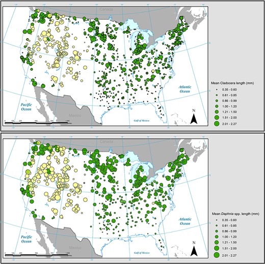
Distribution maps showing mean cladoceran length (top) and mean Daphnia length (bottom) for all lakes sampled. Point magnitude indicates mean length within a single lake. Lakes at elevations below 1000 m are shown as filled green circles, while lakes at elevations above 1000 m are shown as filled yellow circles.
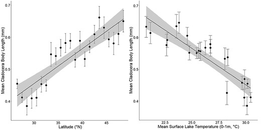
Univariate regression plots showing mean cladoceran length (mm) per 1°N latitude interval (left, R2 = 0.76) and mean cladoceran length (mm) per average surface water temperature (0–1 m, °C) at each 1°N latitude interval (right, R2 = 0.76). The gray area represents 95% confidence interval. Error bars represent standard error. Samples taken at elevations over 1000 m were excluded from this analysis.
Both mean cladoceran body length and mean Daphnia spp. body length displayed a trend of decreasing size with increasing TSI category (Fig. 3). Significant differences in mean cladoceran length (H(3) = 44.84, P < 0.0001) were observed between TSI categories. Post hoc testing revealed that mean cladoceran length was significantly different for oligotrophic lakes (mean = 0.68 mm, standard error = 0.02 mm) compared to mesotrophic (mean = 0.57 mm, standard error = 0.01 mm), eutrophic (mean = 0.54 mm, standard error = 0.01) and hypereutrophic (mean = 0.55 m, standard error = 0.02 mm) lakes. Mean cladoceran length did not differ between mesotrophic, eutrophic and hypereutrophic lakes. Mean Daphnia spp. length also varied significantly (H(3) = 70.0, P < 0.0001) between oligotrophic (mean = 1.02 mm, standard error = 0.03 mm), mesotrophic (mean = 0.91 mm, standard error = 0.02 mm) and eutrophic lakes (mean = 0.81 mm, standard error = 0.02), however no significant difference was observed between eutrophic and hypereutrophic lakes (mean = 0.76 mm, standard error = 0.02 mm) (Fig. 3). Univariate regression between all cladoceran lengths and TSI values produced a significant model (P < 0.001) but with a high degree of variability (R2 = 0.05, Fig. S1).
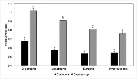
Mean lengths (mm) for all pelagic Cladocera and for Daphnia spp. alone for each TSI tier (± standard error). Superscripted letters represent significant differences between mean lengths for TSI categories (Dunn’s test).
Univariate linear regression between ZC:PC and surface temperature using individual sampling events did not produce a significant model; however a significant trend of decreasing ZC:PC was observed when means were computed per 1°C temperature interval (P < 0.005, R2 = 0.37) (Fig. 4). A trend of increasing ZC:PC was observed across an increasing gradient of latitudinal intervals (P < 0.001, R2 = 0.45) (Fig. 5). Comparison across the four TSI categories revealed significant declines in carbon–carbon ratio of zooplankton to phytoplankton (ZC:PC) with increasing trophic state (H(3) = 160.4, P < 0.0001) (Fig. 6). Post hoc testing showed that Zc:Pc differed significantly between all four TSI categories.
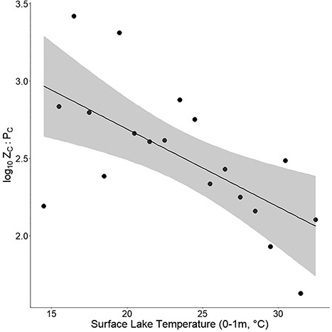
Univariate regression plot between 1°C surface lake temperature intervals and log10-transformed mean ZC:PC (R2 = 0.37). The gray area represents 95% confidence interval. Samples taken at elevations over 1000 m were excluded from this analysis.
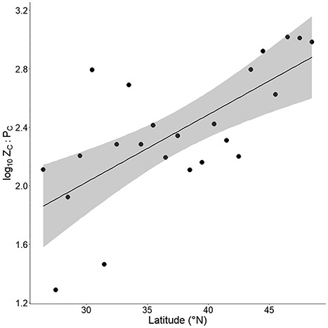
Univariate regression plot between 1°N latitude intervals and log10-transformed mean ZC:PC (R2 = 0.45). The gray area represents 95% confidence interval. Samples taken at elevations over 1000 m were excluded from this analysis.

Mean ZC:PC in each of the four TSI tiers. Letters above the bars represent significant differences between ZC:PC for each TSI category (Dunn’s test). Error bars represent standard error. Samples taken at elevations over 1000 m were excluded from this analysis.
Watershed-scale land use was also compared across TSI categories, revealing significant decreases in percentage of forested area (H(3) = 68.8, P < 0.0001) between each pair of TSI categories (Fig. 7). Significant increases (H(3) = 56.1, P < 0.0001) in percentage of agricultural (crop/pasture) area were observed between oligotrophic lakes (mean = 6.52%, standard error = 0.66%) and both eutrophic (mean = 10.61%, standard error = 0.46%) and hypereutrophic (mean = 12.32%, standard error = 0.74%) lakes, as well as between mesotrophic lakes (mean = 8.34%, standard error = 0.56%) and both eutrophic and hypereutrophic lakes. Percentage of crop/pasture area within individual lake watersheds did not differ significantly between either oligotrophic and mesotrophic lakes or between eutrophic and hypereutrophic lakes.
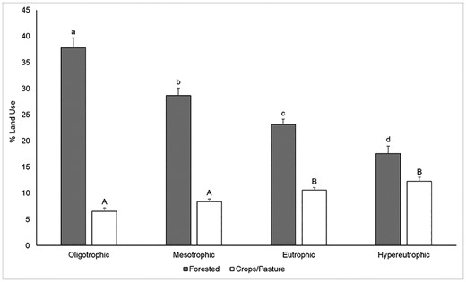
Mean percentage forested and mean percentage crops/pasture per watershed in each of the four TSI tiers. Letters above the bars represent significant differences between percentage land use for each TSI category (α = 0.05, Dunn’s test). Error bars represent standard error. Samples taken at elevations over 1000 m were excluded from this analysis.
The logistic regression of Daphnia dominance against temperature indicated a significant effect of temperature (β = −0.1325, P < 0.001) on the proportion of daphnids in a given sample in the NLA dataset. The results of our model show that the odds of Daphnia spp. dominating the zooplankton of a given lake decrease by a factor of 0.876 with an increase in temperature of 1°C (2.5% CI = 0.846; 97.5% CI = 0.906). A general trend of increasing dominance of copepods and decreasing dominance of cladocerans was observed as TSI increased in 5-unit intervals (Fig. 8).
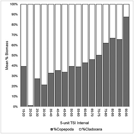
Mean relative contribution to total pelagic crustacean biomass by Copepoda (gray) and Cladocera (white) per 5-unit TSI interval. Samples taken at elevations over 1000 m were excluded from this analysis.
Niche centroid analysis revealed varying environmental optima for different species of cladocerans, including several species within the genus Daphnia (Table II). The smallest commonly occurring cladoceran species in this dataset, Chydorus sphaericus (mean length = 0.28 mm), showed the highest optimum (among evaluated species) for TSI based on chlorophyll-a (78.2), but also showed a relatively high latitude (42.8°N) and relatively low temperature (21.1°C) optima. Another common small cladoceran, Bosmina longirostris (mean length = 0.30 mm) also exhibited a relatively high TSI optimum (69.5), but in contrast to C. sphaericus showed the highest temperature optimum among evaluated species (26.8°C). Within the genus Daphnia, the smallest species in terms of size (D. lumholtzi) exhibited the highest temperature (26.2°C) and the lowest latitude (34.7°N) optima and the highest TSI optimum (67.9). Among commonly occurring Daphnia spp., a gradient was observed between increasing body size and decreasing temperature optima. Although the smallest and largest Daphnia species (D. lumholtzi and D. pulicaria) exhibited the highest and lowest TSI optima, respectively, TSI optima for intermediate sized Daphnia species did not show a consistent pattern.
Locations of niche centroids showing the relationship between frequently occurring small cladoceran species (C. sphaericus and B. longirostris) and species of Daphnia to temperature, latitude and trophic state index based on chlorophyll-a
| Niche centroid optima | |||||
|---|---|---|---|---|---|
| n | Mean Length (mm) | Temperature (°C) | Latitude (°N) | Chl TSI | |
| Chydorus sphaericus | 278 | 0.28 | 21.1 | 42.8 | 78.2 |
| Bosmina longirostris | 583 | 0.30 | 26.8 | 41.6 | 69.5 |
| Daphnia lumholtzi | 57 | 0.66 | 26.2 | 34.7 | 67.9 |
| Daphnia ambigua | 82 | 0.68 | 22.0 | 41.0 | 55.9 |
| Daphnia parvula | 127 | 0.81 | 22.3 | 40.2 | 64.2 |
| Daphnia retrocurva | 107 | 0.95 | 24.0 | 42.0 | 54.8 |
| Daphnia dentifera | 70 | 1.03 | 23.0 | 41.8 | 47.5 |
| Daphnia galeata | 131 | 1.03 | 22.0 | 42.3 | 61.1 |
| Daphnia catawba | 45 | 1.04 | 21.9 | 42.1 | 42.5 |
| Daphnia pulicaria | 109 | 1.29 | 20.4 | 45.4 | 47.9 |
MLR produced a significant model (F (7,1 078) = 39.48, R2 = 0.20, P < 0.001) with four variables (latitude, longitude, elevation and Secchi depth) showing significant correlations (P < 0.001) to mean cladoceran body length (Table III). Mixed models were not significantly more parsimonious than MLR (Table IV). Removal of total nitrogen, total phosphorus and TSI, as well as all three variables at once, were not significantly different from the model that included all environmental variables (Supplementary Tables S1, S2, S3). The mixed model that included only ecoregion (but not individual lake) as a random effect was not significantly different from the full mixed model (chi-square = 0) (Table IV). Comparisons between the full mixed model, two random effects models and the MLR showed the lowest AIC value for the MLR, without accounting for any fixed or random effects in environmental parameters. The lowest BIC value was observed for the linear mixed model where the only random effect included was ecoregion. However, the range in AIC and BIC values between the models was small (Table IV).
Multiple linear regression of mean cladoceran body length and seven environmental variables. Adjusted R2 = 0.197, F7,1 040 = 36.43, P < 0.001
| B | SE | ß | P value | |
|---|---|---|---|---|
| Latitude | 0.00414 | 0.00135 | 0.0896 | <0.001 |
| Longitude | 0.00185 | 0.00052 | 0.1209 | <0.001 |
| Elevation | 0.00007 | 0.00001 | 0.2130 | <0.001 |
| Total nitrogen | 0.00288 | 0.00348 | 0.0253 | 0.4076 |
| Total phosphorus | 0.00006 | 0.00003 | 0.0571 | 0.06818 |
| Secchi depth | 0.02225 | 0.00393 | 0.2112 | <0.001 |
| Trophic state index | 0.00022 | 0.00062 | 0.0136 | 0.7307 |
ANOVA comparing four regression models: the MLR with no random effects (MLR) the mixed model with seven fixed effect variables and individual lakes as the only random effect (Mixed model—lakes), the mixed model with seven fixed effect variables and ecoregion as the only random effect (Mixed model—ecoregions) and the full mixed model (Mixed model—lakes+ecoregions) with seven fixed effect variables and both random effects included
| AIC | BIC | Chi-square | |
|---|---|---|---|
| MLR | 340.29 | 287.79 | |
| Mixed model—lakes | 346.51 | 287.06 | 8.22 |
| Mixed model—ecoregions | 341.43 | 281.98 | 0 |
| Mixed model—lakes+ecoregions | 347.52 | 283.11 | 8.09 |
| AIC | BIC | Chi-square | |
|---|---|---|---|
| MLR | 340.29 | 287.79 | |
| Mixed model—lakes | 346.51 | 287.06 | 8.22 |
| Mixed model—ecoregions | 341.43 | 281.98 | 0 |
| Mixed model—lakes+ecoregions | 347.52 | 283.11 | 8.09 |
DISCUSSION
Cladoceran body size and zooplankton communities
The use of functional traits in ecology lends both generality and predictability to studies in different areas where biogeographical limitations might limit species overlap (McGill et al., 2006). Body size is a functional trait that transcends many ecological functions (Litchman et al., 2013), possibly conveying physiological limitations on growth and/or fitness in interspecies competition. Within lakes and reservoirs of the conterminous USA, cladoceran body size was positively correlated to increasing latitude and decreasing surface temperatures. These results are consistent with Bergmann’s rule and corroborate the findings of Gillooly and Dodson (2000), suggesting that cladoceran body size structure in pelagic lake ecosystems reflects latitude as a function of surface water temperature. Decreased mean body sizes of both cladocerans as a group and populations of Daphnia spp. were significantly associated with increased trophic status. However, multiple regression revealed the complexity of environmental influences on cladoceran body size, with several geographic, temperature-related variables (latitude, longitude and elevation) and one trophic state-related variable (Secchi depth) showing significant relationships to cladoceran body size. These results only partially support our hypothesis that cladoceran body size would be affected by trophic state independently of temperature and latitude. We also saw a change in crustacean community composition over a trophic gradient, from cladoceran dominance in lower TSI lakes to copepod dominance in higher TSI lakes, while the likelihood of Daphnia spp. dominance is predicted to decrease as water temperature increases. These results indicate that both climate warming and eutrophication could result in reduced populations of cladocerans, particularly Daphnia spp.
A shift in zooplankton community structure toward smaller species and a reduced influence of cladocerans could result in restructured aquatic food webs, with unknown consequences to both higher and lower trophic levels. If this were to occur, other components of the zooplankton community (i.e. copepods, rotifers) would likely increase in ecological importance. Cladocerans and copepods often compete for dominance within lake ecosystems, with cladocerans typically grazing more efficiently (Brooks and Dodson, 1965), while copepods are generally superior at escaping predation (Allan, 1976). Cladocerans, particularly large members such as Daphnia spp. (see Table I), typically exhibit higher rates of biomass production than copepods (Peters, 1983). Cladocerans release neonates directly from their pouch, unlike copepods which go through both naupliar and copepodite stages; thus, cladoceran population growth can occur at a faster rate than for copepods (Sommer and Stibor, 2002). Obertegger et al. (2011) observed that microphagous rotifers compete with cladocerans for phytoplankton food sources, suggesting that reduction in cladoceran biomass might open a niche for certain rotifer species. Gradual declines in density of highly efficient herbivore generalists (e.g. Daphnia spp.) and a shift toward copepods and rotifers as the dominant component of the zooplankton community could reduce the strength of top-down controls on phytoplankton population growth, particularly when abiotic factors (i.e. nutrients, light availability) are not limiting. Concurrently, reductions in body size of cladocerans and/or a shift toward dominance by copepods and rotifers could weaken bottom-up supply of available high-quality prey for planktivorous fishes, with negative impacts on sportfish survival (Mayer and Wahl, 1997).
In this study, we also saw reductions in ZC:PC at warmer temperatures and lower latitudes, with significantly higher ZC:PC in lakes classified as oligotrophic in comparison to lakes with higher trophic rankings. A previous study utilizing data from the same survey (the 2012 NLA) showed that the ratio of zooplankton biomass varied proportionally to phytoplankton biomass in oligotrophic lakes but did not vary as phytoplankton biomass increased in eutrophic systems (Yuan and Pollard, 2018). Another recent study using the 2012 NLA data (Sodré et al. 2020) found that land use and nutrient concentrations significantly affected phytoplankton functional guilds but not zooplankton functional guilds, with an association between more inedible and less desirable phytoplankton (i.e. cyanobacteria) and higher nutrient/higher chlorophyll lakes. These findings and results from this study suggest that zooplankton exert little control on phytoplankton biomass, and that phytoplankton growth does not strongly regulate zooplankton in eutrophic and hypereutrophic systems. Jeppesen et al. (2003) found that the effects of the trophic cascade (Carpenter and Kitchell, 1996) are stronger in more productive systems, while primary production in oligotrophic lakes is less sensitive to changes in fish abundance. Elsewhere the absence of large cladoceran taxa, particularly Daphnia spp., has been explained by these species’ vulnerability to predation by planktivorous fish (Luecke et al., 1990; Iglesias et al., 2011; Havens et al., 2015b; Beaver et al., 2019), which tend to be found in higher abundances and throughout longer portions of the growing season at lower latitudes. A broad study of fish feeding guilds in freshwater lakes (Gonzalez-Bergonzoni et al., 2012) showed that lower latitudes supported a higher degree of omnivorous species (as well as higher overall fish density and diversity), suggesting that latitudinal patterns in zooplankton size and community composition are related to latitudinal gradients in fish community structure. Previous studies have also shown higher proportions of planktivorous fish in lakes with elevated nutrient concentrations (Persson et al., 1988). Therefore, it is plausible that high primary production in eutrophic and hypereutrophic lakes, as well as in lakes at lower latitudes, resulted from intense predation on large cladoceran grazers by planktivorous fish. Alternatively, larger zooplankton may have been missed in lakes significantly deeper than 5 m by surface tows performed during the day, when a portion of the zooplankton community likely migrates into deeper water to avoid predation.
Other factors influencing body size
Univariate regression models indicate that both latitude and water temperature are strongly related to zooplankton community size structure, however the influence of trophic state on body size is less clear. The only trophic state variable to show a significant correlation to cladoceran body size was Secchi depth, a measure of water clarity. A previous study of northeastern US lakes found that cladoceran body length was a reliable indicator of water clarity, with larger cladoceran body size significantly related to decreases in chlorophyll-a (Stemberger and Miller, 2003). This effect was likely due to the high clearance capacity of large cladocerans. Interestingly, in this study we found no significant relationship between cladoceran body size and chlorophyll-a. This previously observed pattern may be skewed by large quantities of inedible cyanobacteria in high chlorophyll systems. Secchi depth integrates chlorophyll-a and algal biomass, as well as dissolved organic matter (color) and inorganic particles in the water column into an overall measure of water clarity. A comparison of NLA surveys in 2007 and 2012 found that in general, US lakes are becoming murkier due to increased algal biomass and non-algal organic matter (Leech et al., 2018). This shift has been associated with increased biomass contributions from copepods and rotifers. The fact that Secchi depth, but neither chlorophyll-a nor color independently, was significantly related to cladoceran body size indicates that cladocerans are strongly affected by visual-feeding fish, and lends support to the idea that top-down forces (i.e. fish predation) are more strongly related to cladoceran body size than bottom-up forces (i.e. cultural eutrophication or brownification).
Results from this study show strong relationships between cladoceran body length and both latitude and temperature using 1° N interval means, however more variability was observed in analysis of individual sample points. For example, univariate linear regression using individual data points found a significant negative relationship (P < 0.001) between log-transformed mean Daphnia spp. body length and water temperature. However, temperature only weakly described the variation in Daphnia spp. body length. (Fig. S2). Differences in size structures may result from variations in watershed land use or microclimatic effects resulting from lake morphometry. Our results show that lake trophic state is closely tied to watershed-scale land use practices, as significant differences were observed between lake trophic categories in terms of both percentage of forested areas and percentage of agricultural use. Previous studies have found that increased forest cover is associated with reduced risk of harmful algal blooms and cyanotoxin production (Ghadouani et al., 2006; Marion et al., 2017; Beaver et al., 2018), which may be indirectly beneficial to Daphnia spp. and other cladocerans as they are less tolerant of reduced-quality algal food sources when compared to copepods (Work and Havens, 2003; Ger et al., 2014). The connection between land-use and plankton community dynamics may be useful to land and water management agencies that aim to protect fisheries and native species on a local scale.
Although most lakes at lower latitudes (below about 35°N) contained primarily smaller cladocerans (>1 mm), lakes at higher latitudes are more variable in terms of mean cladoceran body size (Fig. S3). Lakes located at elevations above 1000 m do not show a clear latitudinal gradient in mean cladoceran size or mean Daphnia size (see Fig. 1). This observation suggests that latitudinal patterns observed in lower elevation lakes are likely influenced by temperature—either directly by physiological constraints or indirectly by predator abundance.
Realized body size of individual cladocerans is related to complex environmental, ecological and biological variables (Hart and Bychek, 2011). Extrinsic influences include temperature (negatively associated with body size), food quantity and quality (positively associated with body size), abundance of visual predators (negatively associated with body size) and competition within the community (negatively or positively associated with body size). Intrinsic influences can include physiological limitations and genotypic variability between clonal populations. Interactions between any combination of these of factors are feasible in natural systems and the resulting body size distributions may be highly variable, depending on the species assemblage and/or physical habitat constraints. This is supported by the results of the niche centroid analysis, which found that individual species have varying optima for different environmental variables, which were either temperature- or trophic-related.
Limitations and future directions
One of the strengths of the NLA is the broad range of biomes encompassed within the survey, however trends in water quality may vary by ecoregion (Beaver et al., 2018; Leech et al., 2018). Data from this study were not analyzed separately for different ecoregions because our objective was to examine patterns in zooplankton body size and community composition across a broad area. However, climatic or ecological effects in different regions may help to explain some of the variability in the data. Additionally, there was an uneven distribution of lake types within the study, with a greater percentage of lakes in the northern portion of the study area being natural systems while the majority of sites in the southern portion were man-made reservoirs (although notably almost all Florida sites were natural lakes). Differences in water residence time between these two types of lentic habitats can affect the zooplankton community, potentially favoring copepod dominance when residence time is long (Doubek et al., 2019)—possibly due to enhanced eutrophication and higher fish biomass under low flushing scenarios which would favor the survival of those taxa (i.e. copepods) that are superior at predator avoidance. Reservoirs from the 2012 NLA also tended to be more ecologically disturbed than natural lakes based on significant indicators including zooplankton community, total phosphorus, chlorophyll-a and lakeshore disturbance (Interactive NLA Dashboard, https://nationallakesassessment.epa.gov/).
Because of the nature of the NLA survey—in which individual lakes were sampled only once or twice within a single season—both causes and future projections regarding zooplankton body size and compositional change can only be speculative. A temporal dimension for individual lakes was lacking from this study, aside from a small subset sampled twice within the summer of the same year. Potentially useful data from this study were left out by the need to sample during daylight hours, during which zooplankton are known to perform vertical migration into deeper waters. Given the depth range in sampled lakes (~1–58.5 m), the extent of the zooplankton community captured in 5 m surface tows was likely highly variable. Importantly, no data were collected regarding presence/absence or abundance of potential predators (planktivorous fish). Although fish predation likely plays a strong role in controlling cladoceran body size in many of these lakes, we are unable to show this empirically. Very shallow lakes (<1 m) were excluded from the NLA survey, which may be subject to different environmental constraints on zooplankton body size, such as macrophyte coverage (Gyllström et al., 2005). Very large lakes, including the Great Lakes, were also excluded. Many large, oligotrophic lakes of the world are dominated by copepods (Byron et al., 1984; Barbiero et al., 2001), contrary to findings within our dataset. In deeper lakes, the 5 m vertical tows likely do not capture the full extent of zooplankton habitat. Crustacean zooplankton typically migrate vertically throughout the day, driven by temperature constraints, vulnerability to predation and food availability (William and Overholt, 2019).
Despite these limitations and a high degree of variability in the data, our findings were congruent with those of Gillooly and Dodson (2000), showing that cladoceran body size decreases at lower latitudes and higher temperatures. For cladocerans, the temperature-size rule for ectotherms was upheld. All plankton, by definition, are passively dispersed. Consideration of this aspect of their ecology warrants questions as to whether future changes in size distributions across a latitudinal gradient will be due to shifts in dominant species (i.e. fewer large species and more small species) or phenotypic changes within populations over time. The niche centroid analysis that compared environmental optima between different species of Daphnia suggests that species with similar life cycle and feeding strategies may be both physiologically constrained by ambient water temperature and ecologically constrained in terms of vulnerability to predation. Further studies that incorporate long-term monitoring of lakes over time are needed to investigate specific mechanisms of cladoceran body-size reductions in response to warming temperatures or eutrophication.
CONCLUSIONS
Findings from this study and others (Moore and Folt, 1993; Gillooly and Dodson, 2000; Pinto-Coelho et al., 2005; Alric et al., 2013; Šorf et al., 2015) indicate that under both warming and increased productivity, the average size and total biomass of Daphnia spp. and cladocerans as a group are expected to decrease. These effects are likely to be exacerbated in warm, eutrophic systems at lower latitudes. In conjunction with predictions of warmer climates (Rahmstorf et al., 2007), warmer lakes (Bachmann et al., 2019) increased eutrophication and decreased water clarity (Leech et al., 2018), the results of this study and others suggest that there is a likelihood of seeing corresponding changes in mean cladoceran body size in US lakes under warmer summers in the coming years. We suggest that this important functional trait can be valuable as a measure of assessing the effects of both climate warming and eutrophication in lake ecosystems.
ACKNOWLEDGEMENTS
The authors acknowledge all personnel involved in collection and processing of samples for the 2012 National Lakes Assessment, and Ben Vitanye for his assistance with mapping.
