


Abstract
We have developed an optical photon-counting imaging system, IMONY, as an instrument for short-scale time-domain astronomy. In this study, we utilized a Geiger avalanche photodiode array with a
1 Introduction
Time-domain astronomy has significantly progressed in understanding time-varying or transient astronomical phenomena in recent years. Optical and infrared astronomy has encountered difficulty with short timescales, but this has been overcome with the development of detectors. For instance, high-cadence survey observations with large-area complementary metal-oxide sensor (CMOS) cameras have been successfully implemented (e.g., Sako et al. 2018; Huang et al. 2021). Basically, the timescale of a phenomenon is inversely proportional to the size of its emission region. Observations on very short timescales, milliseconds or less, are primarily used to probe phenomena in the vicinity of compact objects. Achieving high temporal resolution with CMOS is a challenging endeavor.
In such contexts, photon-counting methods are particularly effective. The use of single-photon avalanche diode (SPAD) photon-counting detectors in several previous projects, such as OPTIMA (Stefanescu et al. 2008), SiFAP (Ambrosino et al. 2014), SiFAP2 (Ghedina et al. 2018), SiFAP4XP (Ghedina et al. 2022), Iqueye (Naletto et al. 2019), and Aqueye
We also started developing an optical photon-counting imager that consists of a Geiger avalanche photodiode (GAPD, also known as SPAD) array that is made of a customized multi-pixel photon counter (MPPC). Following the successful first demonstration of Crab pulsar detection with a 35 cm telescope (Nakamori et al. 2021), we commenced a project, Imager of MPPC-based Optical photoN Counter from Yamagata (IMONY), and upgraded the readout and data acquisition system as a prototype. A distinctive feature of our instrument is the capability to realize imaging with monolithic GAPD arrays. The imaging system can have a higher light collection efficiency for point sources than single-pixel systems, as a viewpoint of the containment of the point spread function. Light collection efficiency is essential because photon statistics is often crucial in highly time-resolved observations of fast phenomena.
Another advantage of imaging observation is the stability of photometry. Even for point sources, the position of the image on the focal plane is not stable due to fluctuations caused by the atmosphere and the telescope’s tracking. The image data is helpful to confirm whether the whole spot is contained in the sensor area.
ARCONS (Mazin et al. 2013) also achieves multi-pixel imaging, even with spectroscopy capability, but requires cryogenic cooling and large mechanical structures. In contrast, our system can be operated at room temperature and has the advantage of being compact and easy to handle.
This paper reports on the newly developed readout system and Crab pulsar observation with the Kanata telescope in coordination with radio telescopes as performance tests.
2 System
2.1 Overview
Figure 1 shows an overview of the acquisition system updated in this work. The system consists of roughly two parts: a frontend board (FEB), where the GAPD array sensor is mounted along with amplifiers and comparators, and a data processing board using a field-programmable gate array (FPGA). The FEB was designed to make the system volume smaller than the initial version (Nakamori et al. 2021) that contained power and data bus crates, and a commercial FPGA evaluation board was used to reduce cost. Figure 2 is a photo of the FEB with a ruler to indicate the board size. The sensor is mounted directly on this board, and each sensor channel’s output signal is connected to a wideband amplifier. Each signal is then fed into a comparator to generate a timing signal for photon detection at each pixel. A total of 16 lines are sent in parallel to the FPGA board. A Serial Peripheral Interface (SPI) communication signal from the FPGA also controls the digital-to-analog converter (DAC) to set the comparator threshold. The SPI controls another DAC and the high-voltage output. Power is provided by the FPGA board.
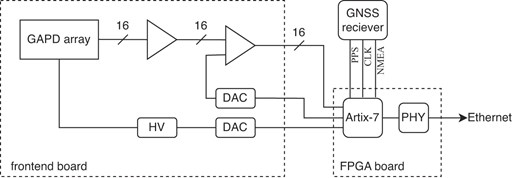
Schematic overview of the system. See text for details.
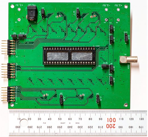
Photo of the frontend readout board.
The FPGA evaluation board is an Artix-7 model that operates with a
We implemented two acquisition modes. The first, the light-curve mode, is the main mode of observation, where we record the arrival time of a photon per pixel as an event list. In the FPGA, a counter is incremented by a 10 MHz clock and is reset each time a PPS is input. Another counter runs simultaneously for the PPS and is initialized to zero at the start of the measurement. When the hit signal is delivered, the values of these two counters determine the relative time at which the photon was detected with an accuracy of 100 ns. Combined with this relative time stamp, the UTC time obtained from the NMEA sentences at the measurement’s start yields the absolute photon detection time. Although a
The second measurement mode, the scaler mode, counts the number of pulses detected during a specified exposure for each channel, namely a count map, where the data is stored in the internal registers. Since the data size is drastically reduced and easier to handle, we implemented this mode for quick health checks during start-up procedures or observations.
The data transfer and command interfaces are implemented using SiTCP (Uchida 2008), which has a high-speed transfer capability using TCP/IP. This work does not realize the full transfer rate since our evaluation board only supports 100BASE-T. As described later, however, it is sufficient for the data transfer rate required for observation. SiTPC can also handle slow control using the User Datagram Protocol (UDP) over the Ethernet, and enable access to the internal bus and resisters, the so-called Remote Bus Control Protocol (RBCP). RBCP is employed to retrieve data acquisition and for DAC control, and to read out the data stored in the registers, such as NMEA information from the GNSS and count numbers obtained by the scaler mode.
2.2 Evaluation
We performed calibration and performance tests in the laboratory, then the signal delay and timing jitter were evaluated. After the calibration of the DACs for the high voltage and threshold settings, we implemented the dark-scan functionality, where we simultaneously measured the dark count rate for all 16 pixels for various threshold values. We obtained a set of dark-scan curves, an example of which is shown in figure 3. Since the intrinsic gain variation among the GAPD cells is 3% (Nakamori et al. 2021), the apparent differences in the cutoff at higher threshold voltages are attributed to the gain and offset variations caused by the characteristics of the amplifier on the FEB. It is also worth noting that channel 9 is known to exhibit a higher dark count rate compared to the others (Nakamori et al. 2021). Finally, we decide the threshold value for operation by finding a common value on the plateau of the dark-scan curves, since the current system version can only set the common threshold voltage via the single DAC chip.
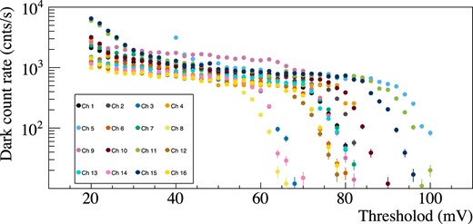
Example of a dark-scan result taken at a temperature of
Using an oscilloscope, we observed a signal delay of 30–40 ns between the input to and output from the comparator. On the other hand, jitter was negligible compared to the delay timescale. Then we irradiated the GAPD array with
3 Observation
3.1 Radio
To obtain the radio timing parameters of the Crab pulsar, which are needed for optical timing analysis, we performed joint observations with the Iitate (Fukushima, Japan) (Tsuchiya et al. 2010) and Usuda (Nagano, Japan) radio telescopes. A summary of the observations is shown in table 1. Iitate Observatory covers the P band with Iitate Planetary Radio Telescope, which consists of dual asymmetric offset parabolas, each with dimensions
Radio observation summary.
| Observatory | Resolution | Start time | Duration | ||
|---|---|---|---|---|---|
| (MHz) | (MHz) | (bits/sample) | (UT) | (hr) | |
| Iitate | 325.1 | 16.0 | 2 | 2021 December 5 10:00:01 | 10.17 |
| Usuda | 2256.0 | 128.0 | 4 | 2021 December 5 15:50:00 | 2.67 |
| Usuda | 8438.0 | 128.0 | 4 | 2021 December 5 15:50:00 | 2.67 |
| Iitate | 325.1 | 16.0 | 2 | 2021 December 6 09:57:01 | 10.64 |
| Iitate | 325.1 | 16.0 | 2 | 2021 December 7 10:00:01 | 10.20 |
| Iitate | 325.1 | 16.0 | 2 | 2021 December 8 09:49:01 | 10.64 |
3.2 Optical
We made optical observations of the Crab pulsar with the Kanata telescope at the Higashi-Hiroshima observatory (Hiroshima, Japan), with an aperture radius of 1.5 m (
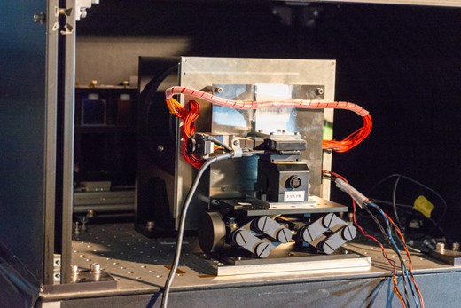
Photograph taken during the installation of the IMONY prototype at the Nasmyth focus of the Kanata telescope. The whole readout system is contained in the aluminum case.
The Crab pulsar was observed from about 14:00 UTC to 19:00 on 2021 December 7. Data taking was divided into many 1–5 min runs. The weather was generally clear, although it was sometimes partially cloudy. We had to repoint the telescope several times during the observation because the FoV of the sensor was so small that the tracking accuracy was not tolerant enough to keep the target in the center of the sensor. We discuss this aspect later.
As mentioned in the previous section, our system is not equipped with any cooling functionality such as a Peltier cooler. Since the front-end circuit board, especially the amplifiers, generates heat, the sensor case has a fan to dissipate the warm air. The temperature and humidity around the GAPD are monitored by a Raspberry Pi using a BME280 sensor. The temperature remained stable at around
During the observation, we took dark-frame data several times by closing the automated mirror facet of the telescope, and also flat-frame data using the observatory’s built-in flat lamp and panel.
4 Analysis and result
4.1 Radio
The goal of radio analysis is to obtain the information needed to phase the visible photon time stamps: the rotation frequency and its derivative, and the reference time of phase zero. The peak of the main radio pulse is defined as phase zero, and the TOA of the first pulse on each observation day,
Timing parameters of the Crab pulsar used in this work.
| Parameter | December 5 | December 7 | Source* |
|---|---|---|---|
| Right ascension | Fixed | JBO | |
| Declination | Fixed | JBO | |
| Ephemeris | DE430 | Fixed | — |
| Epoch | 59553.00000038667824 | 59555.000000320011573 | This work |
| First pulse arrival time | This work | ||
| Pulsar frequency | 29.5893614566(2) | 29.5892979477(2) | JBO |
| Frequency first derivative | JBO | ||
| Frequency second derivative | Fixed | JBO | |
| Dispersion measure (pc cm | 56.7420(10) | Fixed | This work |
JBO: Jodrell Bank Observatory
We applied the coherent de-dispersion method (Hankins & Rickett 1975) to determine the dispersion measure (DM) and correct the frequency-dependent group delay during the propagation. First, we identified several significant GRPs detected simultaneously in both the S- and X-band Usuda data. Then, we determined the best DM so that the pulses were simultaneous in both bands by correcting for the group delay. Figure 5 shows an example of such a coincident GRP; unfortunately, we did not detect a coincident GRP over the X, S, and P bands. We did not use the low-frequency P band to determine the DM since the pulse shape shows a non-negligble time lag due to the slow rise. This effect has been known to be more significant at lower frequencies due to scattering in the interstellar medium (ISM).
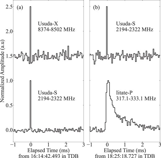
Examples of Crab pulsar GRPs, coincident between the bands. Each pulse shape is normalized, and the baselines are shifted for clarity. (a) X- (above) and S-band (bottom) coincident events used for estimating the DM. (b) X- (above) and P-band (bottom) coincident events used for estimating the lag between the peak time for each.
After the de-dispersion process, we transformed the TOAs recorded in UTC into solar system barycentric dynamical time (TDB) using the PINT package (Luo et al. 2021). The timing model used for the transformation is shown in table 2. Then, we generated time-averaged folded light curves using the pulsar period, its first and second derivatives calculated by extrapolation of values provided by the Jodrell Bank observatory (Lyne et al. 1993).1 After this procedure we excluded time intervals affected by radio-frequency interference. As shown in figure 6, the main pulses were detected in both the P and S bands, while a significant time-averaged signal was not observed in the X band. That is, we could only detect GRPs in the X-band data since the time-averaged emission of the Crab pulsar is fainter at higher frequencies. Finally, we determined

Time-averaged light curves of the Crab pulsar, obtained by Iitate in the P band (top), Usuda in the S band (middle), and Usuda in the X band (bottom). Two pulse cycles are shown. The integration time bin was 10 µs for each.
Unfortunately, we could not obtain S-band data on December 7, the day of the optical observation, so we had to determine
Variation of the ISM also causes the DM and the decay time of the trailing tail of GRPs in the P band. Long-term monitoring of the DM (McKee et al. 2018) shows significant variation, although the day-scale variation was smoothed out in their studies. McKee et al. (2018) also reported that the decay time of the pulse, referred to as the scattering timescale
4.2 Optical
The TOAs of the optical photons in each pixel were reconstructed as absolute UTC times and then converted to TDB using the barycentric correction function in the PINT package. The phase of the Crab pulsar was calculated for each TOA using the radio timing information in table 2, which was obtained as described in subsection 4.1. At the same time, the number of rotations of the Crab pulsar from
We first generated a light curve in all 16 pixels for each. We found the presence of occasional, intermittent rate jumps due to electrical noise in the circuits. The duration of these noise events was not constant, ranging from a few µs to at most
After the data-cleaning procedure for electric noise and cloud cuts, we generated folded phasograms using the timing parameters listed in table 2 and searched for the Crab pulsation for each pixel on a run-by-run basis. The detection criterion was
We then applied the dark count subtraction and flat-frame correction. Figure 7 shows the light curves after the data cleaning. The count rate in the FoV reflects the sky condition. As mentioned in subsection 3.2, the data taking was split into few-minute runs, and the rate drop with a short duration of a few minutes in figure 7 (top) corresponds to the run switching time. The bottom panel shows the photon arrival phase distribution over the observing period. The main peak phase was stable through the night, indicating that our system successfully kept working for several hours. It is also apparent that the count rates around the main peak gradually decrease along with time. We will discuss this point later.
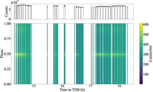
Light curves during the IMONY observation of the Crab pulsar on December 7. The horizontal axis indicates the time, with a unit of Crab turns. (Top) The count rate summed over all 16 pixels. (Bottom) The phase distribution of the detected photons along with time. The phase of the vertical axis is shifted by 0.5 to center the main pulse component.
Figure 8 shows a phasogram of the Crab pulsar with integrating photon events obtained at pulse-detecting pixels. Phase zero corresponds to the timing of the radio’s main pulse. A pulse shape similar to that observed in previous studies was obtained, characterized by an asymmetric main pulse preceding the radio main peak and interpulse. The peak phase of the optical pulse is around
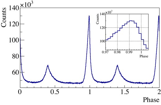
Optical pulse of the Crab pulsar obtained on 2021 December 7. The total exposure of 1.95 hr of data is stacked. The optical peak of the main pulse leads to the radio peak by

We reconstructed the phase-resolved images generated using only the counts of the pulse components. The left and center panels of figure 10 show the on- and off-pulse images of the Crab pulsar, respectively, extracted from the same run data. The spot size in the on-pulse image is consistent with a point-source image with a typical seeing of
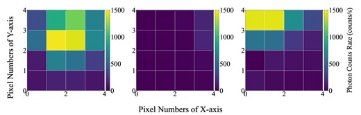
Optical image of the Crab pulsar obtained by the IMONY prototype. Dark subtraction and flat correction were applied, and the exposure time was 3 min for each. (Left) On-pulse image. (Middle) Off-pulse image. (Right) On-pulse image, slightly mispointed.
5 Discussion
The IMONY prototype, which had been upgraded to an FPGA-based data acquisition system, was successfully installed on the Kanata telescope as confirmed by the detection of the Crab pulsar period. The absolute time-stamping capability was also confirmed by the fact that the Crab pulse peak timing was consistent with previous studies. This work marks the first photon-counting observation conducted with the Kanata telescope. Furthermore, we have demonstrated that IMONY worked as an imaging device. In contrast, as noted in our previous paper (Nakamori et al. 2021), the smaller number of pixels and narrow field of view still present a challenge. Even during the observation of this work, approximately 60 min after the start of the observation the object’s image was no longer within the field of view. For example, in figure 7 (bottom), it is clear that the main pulse component was gradually disappearing before turns
Regarding the absolute timing of the optical peak, our results of the peak timing depend on the uncertainty of
As described in section 2, the data transfer rate of the system was limited by the 100BASE-T capability. During the Crab observation in this work, the raw data rate was typically less than 2 Mbit s
In the case of observations like the GRPs of the Crab pulsar, where the observations must be continued while awaiting the occurrence of a phenomenon, it is necessary to implement continuous tracking over an extended period. It is anticipated that more careful pointing analysis than previously conducted would enhance the tracking accuracy. However, this approach is both laborious and ineffective. One potential solution would be to increase the size of the sensor and expand the field of view. A 64-pixel sensor system has already been developed and is currently undergoing testing (Hashiyama et al. 2024). Due to this context, we do not focus on the accuracy of the photometry in this prototype since the fraction of the detected photons was not stable during the observation. The imaging capability turned out to be important since we were able to identify that the drop in the flux was due not to the source variation but to the telescope’s mispointing. We intend to commence regular operation of IMONY as soon as possible, utilizing the system as a new system for optical photon-counting astronomy.
Funding
This work was supported by JSPS KAKENHI Grant Numbers JP20H10940 and JP23H01194, the Yamada Science Foundation, and the NAOJ Research Coordination Committee (NAOJRCC-2101-0103).
Data availability
The data underlying this article are available on request from the authors.
Acknowledgments
The authors express their sincere gratitude to Dr. A. Hayato for her contribution in designing the jig of the system. We also thank the anonymous referee for careful reading and giving helpful comments to improve the manuscript.
