


Abstract
We have carried out the NH3(J, K) = (1, 1), (2, 2), and (3, 3) mapping observations toward the Galactic infrared bubble N49 (G28.83−0.25) using the Nobeyama 45 m telescope. Three NH3 clumps (A, B, and C) were discovered along the molecular filament with the radial velocities of ∼96, 87, and 89 km s−1, respectively. The kinetic temperature derived from the NH3(2, 2)/NH3(1, 1) shows Tkin = 27.0 ± 0.6 K enhanced at Clump B in the eastern edge of the bubble, where position coincides with massive young stellar objects (MYSOs) associated with the 6.7 GHz class II methanol maser source. This result shows the dense clump is locally heated by stellar feedback from the embedded MYSOs. The NH3 Clump B also exists at the 88 km s−1 and 95 km s−1 molecular filament intersection. We therefore suggest that the NH3 dense gas formation in Clump B can be explained by a filament–filament interaction scenario. On the other hand, NH3 Clumps A and C at the northern and southern sides of the molecular filament might be the sites of spontaneous star formation because these clumps are located ∼ 5–10 pc away from the edge of the bubble.
1 Introduction
Ionized hydrogen (H ii) regions are formed by the ultraviolet radiation from OB-type stars. They are known to be sites of triggered star formation from previous works of observations and theories (e.g., Elmegreen 1998) and are also identified as “interstellar bubbles” (e.g., Castor et al. 1975; Weaver et al. 1977). For example, the Galactic Legacy Infrared Mid-Plane Survey Extraordinaire (GLIMPSE) by the Spitzer space telescope found ∼ 600 infrared bubbles in the Galactic plane (|$|l| \le {65^{\circ}}, |b| \le {1^{\circ}}$|: Churchwell et al. 2006, 2007). Most of them are H ii regions excited by OB-type stars inside the bubbles (Deharveng et al. 2010). Two star formation scenarios regarding bubbles have recently been discussed as “collect-and-collapse” (Deharveng et al. 2010) and “cloud–cloud collisions” (Fukui et al. 2021) based on their morphology and distributions of parent clouds. The former is shock compression by the expansion of H ii regions which triggers second generation star formation at the edge of the bubble (e.g., Elmegreen & Lada 1977; Whitworth et al. 1994; Deharveng et al. 2005; Hosokawa & Inutsuka 2006; Zavagno et al. 2006, 2007; Dale et al. 2007; Thompson et al. 2012; Xu & Ju 2014; Palmeirim et al. 2017; Li et al. 2019; Luisi et al. 2021). The latter is when two clouds with different sizes collide, triggering the formation of exciting stars and forming arc-like morphology (e.g., Habe & Ohta 1992; Hasegawa et al. 1994; Higuchi et al. 2014; Torii et al. 2015; Baug et al. 2016; Fukui et al. 2018; Ohama et al. 2018; Fujita et al. 2019; Koide et al. 2019; Kohno et al. 2021b; Yamada et al. 2021; Enokiya & Fukui 2022). These scenarios are possibly related to infrared bubbles however, the dominant mechanism remains unclear.
N49 (also known as G28.83−0.25) is an infrared bubble at |$(l,b) \sim ({28{_{.}^{\circ}}83}, {-0{^{\circ}_{.}}23})$| in the Galactic plane (Zavagno et al. 2010), which is identified as a “closed bubble” based on AKARI 9 μm infrared morphology (Hattori et al. 2016; Hanaoka et al. 2019, 2020). It has been studied as a representative “wind-blown bubble” (Everett & Churchwell 2010). The distance to N49 from the solar system is 5.07 kpc, which is associated with the Scutum Arm (Dirienzo et al. 2012; Dewangan et al. 2017). Figure 1a shows the three-color composite image of the Spitzer space telescope (Werner et al. 2004). Blue, green, and red present the 3.6 μm, 8.0 μm, and 24 μm images, respectively. These bands trace the thermal emission from the stars, polycyclic aromatic hydrocarbons (PAH) emission in the photo-dissociation region (e.g., Draine & Li 2007; Draine 2003), and hot dust heated by OB-type stars (e.g., Carey et al. 2009), respectively. Figure 1b presents the close-up image of the N49 bubble. White contours indicate the Very Large Array (VLA) 1.4 GHz continuum image, which traces distributions of the ionized gas. The distribution of the ionized gas coincides with the hot dust emission traced by the Spitzer 24 μm image. Young stellar objects YSO |$\#$|1, YSO |$\#$|3, and the ultra-compact H ii region (UC H ii) exist at the bubble’s eastern edge (see figure 18 in Deharveng et al. 2010). Previous studies reported that YSO |$\#$|3 is associated with the 6.7 GHz class II methanol maser embedded in the massive YSOs and referred to as extended green objects (EGOs: Cyganowski et al. 2008, 2009; see also the data base of astrophysical masers; Ladeyschikov et al. 2019).1 Figure 1c shows the 13CO J = 1–0 peak intensity map obtained by the Nobeyama 45 m telescope (Umemoto et al. 2017; Torii et al. 2019). The optically thinner 13CO J = 1–0 can trace a molecular hydrogen density of |$n(\rm {H_2}) \sim 10^3\:$|cm−3 (e.g., Solomon et al. 1979; Nagahama et al. 1998; Kawamura et al. 1998; Jackson et al. 2006; Torii et al. 2019). Thus, it is appropriate to study the large-scale structure in the surroundings of the dense gas. 13CO has a filamentary structure and arc-like morphology around the ionized gas at the eastern side of the N49 bubble (see also figure 12 in Yan et al. 2016).
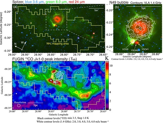
(a) Spitzer three-color composite image of the infrared bubble N49. Blue, green, and red show 3.6 μm, 8.0 μm, and 24 μm, respectively. The yellow enclosed area indicates the NH3 mapping region of our project. (b) The close-up image of panel (a). White contours show the VLA 1.4 GHz continuum image (Helfand et al. 2006). The lowest contour level and intervals are 2 and 1 mJy beam−1, respectively. The ultra-compact H ii region, YSO #1, and YSO #3 are labeled (see Figure 18 in Deharveng et al. 2010 and Watson et al. 2008). (c) The peak intensity (TMB) map of 13CO J = 1–0 obtained by the FUGIN project (Umemoto et al. 2017; Torii et al. 2019). The black lowest contour level and intervals are 3.5 and 1.0 K, respectively. White contours show the VLA 1.4 GHz continuum image. The white contour levels are 2.0, 3.0, 4.0, 5.0, and 6.0 mJy beam−1. The white cross indicates the position of the 6.7 GHz class II methanol maser source (Cyganowski et al. 2008, 2009).
Previous studies of the N49 bubble suggested triggering of star formation by an expanding H ii region (Watson et al. 2008; Dirienzo et al. 2012). Xu et al. (2019) performed CO observations toward the molecular filament and bubble. They argue that feedback from the H ii region affects star formation and helps to drive the turbulence in the filament. On the other hand, Dewangan, Ojha, and Zinchenko (2017) found two different radial velocity filaments associated with the bubble. They argued that the filament–filament collision scenario could explain the massive star formation at the edge of the bubble.
Star formation scenarios are discussed in previous works, while the dense gas formation mechanism related to star formation of the N49 bubble and the molecular filament is not yet clear. The NH3 emission can trace dense gas [|$n(\rm {H_2}) \gtrsim 10^{4}\:$|cm−3] and derive the kinetic temperature of molecular gas because of the excitation of the NH3 inversion transitions in the lowest metastable rotational energy states at low temperatures. It also allows us to derive the optical depth and column density, using the splitting of the inversion transitions into different hyperfine structure components around 23 GHz (e.g., Cheung et al. 1968, 1969; Morris et al. 1973; Walmsley & Ungerechts 1983; Ho & Townes 1983). Previous studies of NH3 observations toward the N49 bubble focused only on the dust clumps identified by the APEX Telescope Large Area Survey of the Galaxy (ATLASGAL: e.g.,Wienen et al. 2012). In order to trace the large-scale structure of the environment around the dust clumps, we performed mapping observations (of about 30 pc) of the NH3 inversion transition of (J, K) = (1, 1), (2, 2), and (3, 3) using the Nobeyama 45 m telescope (see the yellow enclosed area in figure 1a and 1c). J and K are the quantum number of the total angular momentum and their projection along the molecular axis (Ho & Townes 1983). In this paper, we adopted the energy levels of each NH3 transition from the Jet Propulsion Laboratory (JPL) spectral line catalog (Pickett et al. 1998).2 This paper is structured as follows: section 2 introduces observations and the archive data; section 3 presents the NH3 results; in section 4, we discuss dense gas and star formation scenarios in three NH3 clumps along the molecular filament, and in section 5, we show a summary of this paper.
2 Observations
2.1 The KAGONMA project: NH3 mapping observations using the Nobeyama 45 m telescope
We carried out NH3(J, K) = (1, 1), (2, 2), and (3, 3) mapping observations using the Nobeyama 45 m telescope led by Kagoshima University. Our NH3 survey project is called “KAGONMA” (“Kagoshima galactic object survey with the Nobeyama 45-metre telescope by mapping in ammonia lines”) and makes use of survey papers on the Galactic Center and massive star forming regions already published (Nagayama et al. 2007, 2009; Toujima et al. 2011; Chibueze et al. 2013; Nakano et al. 2017; Burns et al. 2019; Murase et al. 2022; Kohno et al. 2022; Y. Hirata et al. in preparation).3 We utilized the dual-polarization and the multi-ON–OFF switching (three ON points per one OFF point) mode. The observational period was from 2014 December to 2015 June (PI T. Omodaka: BU145001).4 The half-power beam width (HPBW) and grid spacing was 75″ at 23 GHz and |${37{^{\prime \prime}_{.}}5}$|, respectively. We used the High Electron Mobility Transistor (HEMT) receiver named H22 at 22 GHz as the front end. The pointing accuracy was checked within 5″ by observing the H2O maser source OH 43.8−0.1 |$(\alpha _{\rm J2000.0}, \delta _{\rm J2000.0})=({19^{\rm h}11^{\rm m}54{^{\rm s}}},{+09{^{\circ}_{.}}35^{\prime }55^{\prime \prime }})$| before starting observations. The FX-type digital spectrometer was used as the back-end system. It is named the Spectral Analysis Machine of the 45 m telescope (SAM 45: Kuno et al. 2011; Kamazaki et al. 2012). The system noise temperature (Tsys) including the atmosphere was 150–250 K during observations. We used eight intermediate frequencies (IFs) to observe the NH3(J, K) = (1, 1), (2, 2), (3, 3), and H2O maser with the dual-polarization simultaneously. Each IF’s frequency bandwidth and resolution were 125 MHz and 30.52 kHz corresponding to the velocity coverage of 1600 km s−1 and spacing of 0.39 km s−1 at 23 GHz, respectively. The chopper wheel method was adopted to calibrate to the intensity of the antenna temperature (|$T_{\rm a}^*$|: Ulich & Haas 1976; Kutner & Ulich 1981). We used the NEWSTAR software package (Ikeda et al. 2001) to make the cube file from the raw data.5 We subtract baselines with a first-order polynomial function from the spectra. The baseline ranges were set up as emission-free channels of each spectrum. Then, we applied the hanning smoothing (width = 5) in the velocity domain to improve the signal-to-noise ratio. The antenna temperature was converted to the main-beam temperature (TMB) using the relation of |$T_{\rm MB}= T_{\rm a}^*/\eta _{\rm MB}$|. The main-beam efficiency (ηMB) is 0.835, the average value of two channels of the H22 receiver in the Nobeyama 45 m telescope. The kinetic temperature and physical parameters are not dependent on the main-beam efficiency because we can derive them from intensity ratios of different transitions around 23 GHz obtained by the same instrument of a radio telescope.
The rms noise level for the final data was ∼0.03 K at the TMB scale (corresponding to ∼0.025 K at the |$T_{\rm a}^*$| scale). The parameters of our NH3 data are summarized in table 1.
Properties of our observations.
| Telescope | Molecule | Transition | Eu/kB | ν0 | Receiver | Grid | HPBW | Velocity | RMS noise |
|---|---|---|---|---|---|---|---|---|---|
| [K] | [GHz] | spacing | resolution | level | |||||
| (1) | (2) | (3) | (4) | (5) | (6) | (7) | (8) | (9) | (10) |
| Nobeyama 45 m | NH3 | (J, K) = (1, 1) | 23.3 | 23.694 | H22 | |${37{^{\prime \prime}_{.}}5}$| | 75″ | 0.39 km s−1 | ∼0.03 K |
| NH3 | (J, K) = (2, 2) | 64.4 | 23.723 | H22 | |${37{^{\prime \prime}_{.}}5}$| | |${75^{\prime \prime }}$| | 0.39 km s−1 | ∼0.03 K | |
| NH3 | (J, K) = (3, 3) | 123.5 | 23.870 | H22 | |${37{^{\prime \prime}_{.}}5}$| | |${75^{\prime \prime }}$| | 0.39 km s−1 | ∼0.03 K |
Columns: (1) Telescope name. (2) Molecules. (3) Transitions; J and K are the quantum number of total angular momentum and their projection along the molecular axis, respectively. (4) Upper energy levels; (Eu) of inversion transitions above the ground state divided by the Boltzmann constant; (kB). (5) Rest frequency (ν0). (6) Receiver name. (7) Grid spacing of the multi-ON–OFF switching observations. (8) Half-power beam width. (9) Velocity resolution. (10) Root mean square noise level of the TMB scale.
2.2 Archival data
We utilized the 13CO J = 1–0 data by comparing it with NH3 spatial and velocity distributions. It was obtained by the FOREST Unbiased Galactic plane Imaging survey with the Nobeyama 45 m telescope (FUGIN6: Umemoto et al. 2017; Kohno et al. 2018; Nishimura et al. 2018, 2021; Torii et al. 2018, 2019, 2021; Sofue et al. 2019; Nakanishi et al. 2020; Fujita et al. 2021; Kohno et al. 2021a; Sato et al. 2021). The FUGIN CO survey adopted the on-the-fly (OTF) mapping mode (Sawada et al. 2008) and used the FOur-beam REceiver System on the 45 m Telescope (FOREST) with the four-beam, dual-polarization, side-band separating receiver (Minamidani et al. 2016; Nakajima et al. 2019). The HPBW and effective resolution convolved by the Gaussian kernel function are 15″ and 21″ at 110 GHz, respectively. The effective velocity resolution is 1.3 km s−1. Smoothing the data cube using a Gaussian kernel function resulted in a resolution of ∼40″. The rms noise level is ∼0.3 K at the main beam temperature scale. We used the 1.4 GHz (= 20 cm) radio continuum image with the angular resolution of ∼6″ taken from the Multi-Array Galactic Plane Imaging Survey (MAGPIS) with VLA (White et al. 2005; Helfand et al. 2006). The 1.4 GHz radio continuum image is useful to investigate the free–free emission corresponding to the ionized gas from H ii regions. We also obtained the archive data of the Spitzer Space telescope with the wavelengths of 3.6 μm, 8 μm (Benjamin et al. 2003; Churchwell et al. 2009), and 24 μm (Carey et al. 2009). Additionally, the 870 μm dust continuum image is taken from ATLASGAL7 (Schuller et al. 2009). The fits’ cubes were taken from the MAGPIS web page.8
2.3 Software packages
In this paper, we used the following software packages to create the maps, extract the spectra, and calculate physical parameters (Astropy: Astropy Collaboration 2013, 2018, NumPy: van der Walt et al. 2011, Matplotlib: Hunter 2007, IPython: Perez & Granger 2007, Miriad: Sault et al. 1995, and APLpy: Robitaille & Bressert 2012).
3 Results
3.1 NH3 spatial distributions
Figure 2 shows the peak temperature map of the main line in (a) NH3(J, K) = (1, 1), (b) NH3 (2, 2), and (c) NH3 (3, 3). The white contours present the ionized gas distribution traced by the VLA 1.4 GHz radio continuum image. We identified three clumps in the NH3 (1, 1) line as revealed by the intensity peaks along the molecular filament (figure 2a). Hereafter, we called these clumps “Clump A,” “Clump B,” and “Clump C.” The NH3 (1, 1) peak in Clump B exists on the eastern side of the N49 bubble offset from the ionized gas. We detected NH3 (2, 2) emission in Clumps A, B, and C (figure 2b). The NH3 (2, 2) emission is enhanced in Clump B at the eastern edge of the bubble (figure 2c).
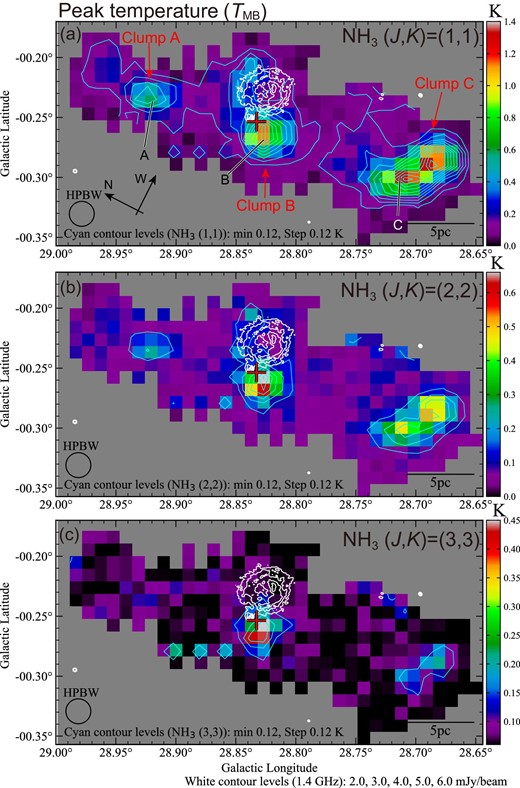
Peak intensity (TMB) map of (a) NH3(J, K) = (1, 1), (b) NH3 (2, 2), and (c) NH3 (3, 3). The lowest cyan contour level and intervals of NH3 are 0.12 K (∼4σ) and 0.12 K (∼4σ), respectively. Three NH3 clumps are labeled in panel (a). A, B, and C show the positions of the spectra in figure 3. The white contour levels of the VLA 1.4 GHz continuum image are 2.0, 3.0, 4.0, 5.0, and 6.0 mJy beam−1. The red cross indicates the position of the 6.7 GHz class II methanol maser source (Cyganowski et al. 2008, 2009).
Figure 3 shows the NH3 peak spectrum at Clumps A, B, and C. The locations of each spectrum are labeled in figure 2a. In the NH3 (1, 1) emission, the main line exists as the central velocity of each spectrum. We also detected the hyper-fine structures of the inner (F1 = 1 → 2, 2 → 1) and outer (F1 = 1 → 0, 0 → 1) satellite lines, where F1 is the quantum number of the angular momentum, contributing to the nitrogen nuclear-spin. The intensity peak of NH3 (1, 1) exists at Clump C, while NH3 (3, 3) has a peak intensity at Clump B. We derived the peak temperature, peak velocity, and full-width half maximum (FWHM: hereafter, we call it the line width) obtained by a Gaussian fitting toward the main line of each profile. The profile parameters are summarized in table 2. The errors are the standard deviations of each fitting parameter.

NH3 spectra at A |$(l,b)=({28{_{.}^{\circ}}921}, {-0{^{\circ}_{.}}237})$|, B |$(l,b)=({28{_{.}^{\circ}}827}, {-0{^{\circ}_{.}}268})$|, and C |$(l,b)=({28{_{.}^{\circ}}712}, {-0{^{\circ}_{.}}299})$|. These positions are also presented in figure 2a. Red lines show the results from a Gaussian function fitted to the emission at the main component. NH3 (1, 1) emissions include four satellite components of F1 = 1 → 0, F1 = 1 → 2, F1 = 2 → 1, and F1 = 0 → 1 (from left to right on the velocity axis).
NH3 spectra parameters of the main line in each NH3 clump.*
| Name | l | b | Transition | TMB | vLSR | Δv |
|---|---|---|---|---|---|---|
| [°] | [°] | (J, K) | [K] | [km s−1] | [km s−1] | |
| (1) | (2) | (3) | (4) | (5) | (6) | (7) |
| A | 28.921 | −0.237 | (1, 1) | 0.61 ± 0.02 | 96.4 ± 0.04 | 2.3 ± 0.10 |
| (2, 2) | 0.22 ± 0.01 | 96.4 ± 0.05 | 1.9 ± 0.11 | |||
| (3, 3) | 0.10 ± 0.01 | 95.6 ± 0.12 | 2.6 ± 0.29 | |||
| B | 28.827 | −0.268 | (1, 1) | 1.09 ± 0.04 | 86.9 ± 0.02 | 2.5 ± 0.10 |
| (2, 2) | 0.56 ± 0.007 | 86.9 ± 0.02 | 2.8 ± 0.04 | |||
| (3, 3) | 0.39 ± 0.007 | 86.8 ± 0.03 | 3.3 ± 0.06 | |||
| C | 28.712 | −0.299 | (1, 1) | 1.26 ± 0.05 | 88.7 ± 0.04 | 1.9 ± 0.10 |
| (2, 2) | 0.47 ± 0.01 | 88.5 ± 0.03 | 1.8 ± 0.06 | |||
| (3, 3) | 0.11 ± 0.008 | 88.4 ± 0.19 | 4.9 ± 0.44 |
*Columns: (1) Name of each spectra. (2) Galactic longitude. (3) Galactic latitude. (4) Rotational transition. (5) Peak temperature (TMB). (6) Peak velocity by a single Gaussian fitting. (7) The line width (|$2 \sigma \sqrt{2 \ln 2}$|) of spectra by a Gaussian fitting, where σ is the standard deviation of the line profile. The errors are the standard deviations of each fitting parameter.
3.2 Three NH3 clumps with the different radial velocity
Figures 4, 5, and 6 show the NH3 (1, 1), NH3 (2, 2), and NH3 (3, 3) velocity channel maps, respectively. Clumps A, B, and C have an intensity peak of all transitions at 96–97 km s−1 [panel (i) in figures 4–6], 85–88 km s−1 [panels (b) and (c) in figures 4–6], and 88–90 km s−1 [panel (d) in figures 4–6], respectively. Clump A and B connect with the diffuse NH3 (1, 1) emission of 94–97 km s−1 (figures 4h and 4i). To investigate the velocity field of each clump in more detail, we made the peak velocity and line width map of the NH3 (1, 1) main line obtained by a Gaussian fitting toward a profile at each pixel.
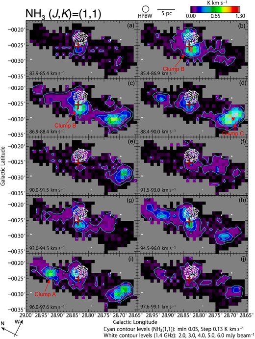
Velocity channel map of NH3(J, K) = (1, 1). The lowest cyan contour level and intervals are 0.05 K km s−1 (∼3σ) and 0.13 K km s−1 (∼8σ), respectively. The red cross and white contours are the same as in figure 2a. The white contour levels of the VLA 1.4 GHz continuum image are 2.0, 3.0, 4.0, 5.0, and 6.0 mJy beam−1.
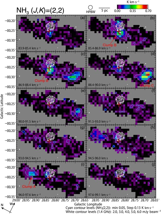
Same as figure 4, but for NH3(J, K) = (2, 2).
Figures 7a and 7b shows the peak velocity and line width maps of the NH3 (1, 1) main line, respectively. Clumps A, B, and C have different radial velocities at ∼96, ∼87, and ∼89 km s−1 (figure 7a). We also find the 100 km s−1 velocity component at |$(l,b) \sim ({28{_{.}^{\circ}}72}, {-0{^{\circ}_{.}}24})$| around the northwestern side of Clump C. The line width of Clump A is ∼2.3 km s−1. Clump B has a large line width of ∼3.0 km s−1 around the methanol maser source shown by the cross mark. Finally, we point out that Clump C has a uniform line width of ∼2.0 km s−1.

Same as figure 4, but for NH3(J, K) = (3, 3).
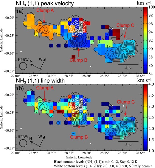
(a) Peak velocity and (b) velocity width maps of the NH3(J, K) = (1, 1) line resulting from a Gaussian function fitted to the emission within pixels above 0.12 K (>4σ). The black contours show the NH3(J, K) = (1, 1) peak intensity. The lowest black contour level and intervals are 0.12 K (∼4σ). The red cross and white contours are the same as in figure 2a. The white contour levels of the VLA 1.4 GHz continuum image are 2.0, 3.0, 4.0, 5.0, and 6.0 mJy beam−1.
3.3 Physical properties of NH3 clumps
Figure 8 presents the kinetic temperature distribution. The center of Clump A has Tkin = 17.7 ± 0.1 K, and the northern part at |$(l,b)\sim ({28{_{.}^{\circ}}96}, {-0{^{\circ}_{.}}206})$| has a high temperature of Tkin = 26.4 ± 0.3 K. Clump B around the methanol maser source is enhanced of Tkin = 27.0 ± 0.6 K. This peak value is consistent with Tdust ∼ 27 K obtained by the Herschel continuum image (see figure 8a in Dewangan et al. 2017). Clump C has uniform temperature distribution of Tkin ∼ 14–18 K.
Figure 9 shows the NH3 total column density map. Clump B has a high column density of (9.1 ± 0.4) × 1015 cm−2 at |$(l,b) = ({28{_{.}^{\circ}}837}, {-0{^{\circ}_{.}}247})$|, which coincides with the UC H ii region. In contrast, Clumps A and C have lows of |$(1.8^{+0.09}_{-0.08}) \times 10^{15}\:$|cm−2 and ∼(3.7 ± 0.3) × 1015 cm−2, respectively. These values correspond to ∼3.6 × 1023 cm−2, ∼7.2 × 1022 cm−2, and ∼1.5 × 1023 cm−2 of the H2 column density, respectively. We used the N(NH3)-to-N(H2) conversion factor of X(NH3) = 2.5 × 10⁻⁸ derived from the massive star-forming regions in the Galactic plane (Urquhart et al. 2015). The peak H2 column density around the methanol maser source is a factor of 4 larger than ∼9 × 1022 cm−2 obtained by the Herschel dust continuum image (Dewangan et al. 2017).
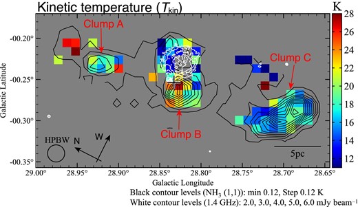
Kinetic temperature map obtained by the (2, 2)/(1, 1) integrated intensity ratio above the 3σ noise level. The black contours show the NH3(J, K) = (1, 1) peak intensity. The lowest black contour level and intervals are 0.12 K (∼4σ). The cross mark and white contours are the same as in figure 2a. The white contour levels of the VLA 1.4 GHz continuum image are 2.0, 3.0, 4.0, 5.0, and 6.0 mJy beam−1.
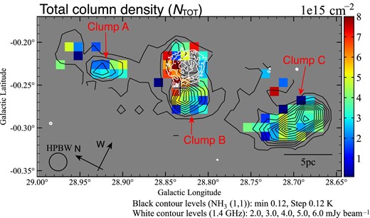
NH3 total column density map above the 3σ noise level. The contours show the NH3(J, K) = (1, 1) peak intensity. The lowest black contour level and intervals are 0.12 K (∼4σ). The cross mark and white contours are the same as in figure 2a. The white contour levels of the VLA 1.4 GHz continuum image are 2.0, 3.0, 4.0, 5.0, and 6.0 mJy beam−1.
Physical parameters in each NH3 clump.*
| Name | Radius | τ(1, 1, m) | Trot | Tkin | Ntot(NH3) | N(H2) | MLTE |
|---|---|---|---|---|---|---|---|
| [pc] | [K] | [K] | [cm−2] | [cm−2] | [M⊙] | ||
| (1) | (2) | (3) | (4) | (5) | (6) | (7) | (8) |
| Clump A | 1.6 | 1.4 ± 0.6 | 16.5 ± 2.0 | 19.2 ± 3.0 | (2.9 ± 1.0) × 1015 | (1.2 ± 0.4) × 1023 | 2.0 × 10⁴ |
| Clump B | 2.8 | 1.6 ± 0.7 | 15.4 ± 3.9 | 17.9 ± 5.2 | (4.3 ± 2.2) × 1015 | (1.7 ± 0.9) × 1023 | 9.5 × 10⁴ |
| Clump C | 2.8 | 1.5 ± 0.6 | 14.6 ± 1.5 | 16.5 ± 2.1 | (3.2 ± 1.2) × 1015 | (1.3 ± 0.5) × 1023 | 7.1 × 10⁴ |
Columns: (1) Clump name. (2) The clump radius defined above 3σ of the NH3 (1, 1) and NH3 (2, 2) emission. (3) The mean value of optical depth. (4) The mean value of rotational temperature. (5) The mean value of the kinetic temperature. (6) The mean value of the total NH3 column density. (7) The mean value of H2 column density. (8) The total LTE mass of a clump. The errors are derived by the standard deviation of the mean value in each clump.
4 Discussion
4.1 Distributions of cold dust condensations and star formation in NH3 clumps
Figure 10 shows the NH3 distributions presented by pink contours superposed on the 870 μm dust continuum image. We point out Clumps A, B, and C corresponding to the dust condensations of AGAL 028.922−00.227,9 AGAL 028.831−00.252,10 and AGAL 028.707−00.294,11 respectively. These dust clumps were identified by the ATLASGAL survey (Csengeri et al. 2014; Urquhart et al. 2014). The dust peak exists at |$(l,b) \sim ({28{_{.}^{\circ}}96}, {-0{^{\circ}_{.}}20})$|, which is the northern side of Clump A. The NH3 peaks of Clump B coincide with three dust condensations of #1, #3, and #4 along with the edge of the N49 bubble (see also figure 18 in Deharveng et al. 2010).
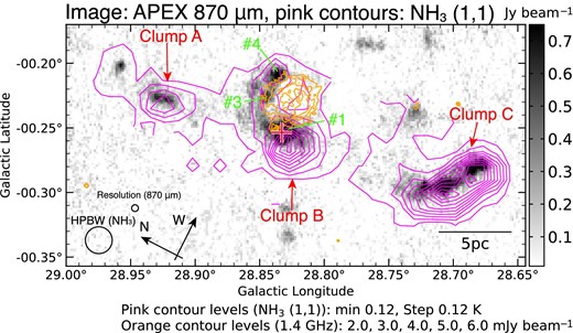
NH3(J, K) = (1, 1) peak intensity shown as pink contours superposed on the APEX 870 μm continuum image. The lowest pink contour level and intervals are 0.12 K (∼4σ). The red cross is the same as in figure 2a. The orange contour levels of the VLA 1.4 GHz continuum image are 2.0, 3.0, 4.0, 5.0, and 6.0 mJy beam−1. #1, #3, and #4 indicate the dust condensations identified by Deharveng et al. (2010).
Figure 11 presents the distributions of YSOs identified by Dirienzo et al. (2012). The image and pink contours show the Spitzer 8 μm and peak intensity of NH3 (1, 1), respectively. Dirienzo et al. (2012) classified YSOs as “Stage I, Stage II, and Stage III” with their evolutional stage defined by Robitaille et al. (2006). Clumps A and C have Stage I YSOs shown in blue circles. Clump B has Stage I YSOs at the edge and inside the bubble. Stage II YSOs exist on the eastern side of Clump B. We suggest that the low-mass star formation proceeds at each NH3 clump in the molecular filament because YSOs exist at each dense clump. Clumps A and C exist at ∼5 pc and ∼10 pc away from the edge of the bubble traced by the 1.4 GHz radio continuum image. Therefore, we propose that these clumps might not be affected by the external shock compression or ionization from the N49 bubble, but the sites of spontaneous star formation. Clump C has low kinetic temperatures of 14–18 K (figure 8) and the uniform line width of ∼2.0 km s−1 (figure 7b), while it includes NH3 dense gas, cold dust condensation, and Stage I YSOs (figure 10). We suppose that they show signatures of the early stage of star formation in Clump C. Clumps A and C are not detected in the radio continuum emission even though they contain dust condensations and YSOs. Therefore, these clumps might be at a more initial stage or on a smaller scale of star formation than Clump B.
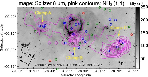
YSO distributions superposed on the Spitzer 8 μm continuum image. Pink contours indicate the NH3(J, K) = (1, 1) peak intensity. The lowest pink contour level and intervals are 0.12 K (∼4σ). Blue, green, and red circles show the Stage I, Stage II, and Stage III YSOs identified by Dirienzo et al. (2012) based on the classification model of Robitaille et al. (2006).
4.2 Impact of the N49 bubble to the NH3 clump
The NH3 (1, 1) main line has a large line width of 3.8 ± 0.3 km s−1 at |$(l,b) = ({28{_{.}^{\circ}}837},{-0{^{\circ}_{.}}226})$|, which corresponds to the northern interface of Clump B and ionized gas (figure 7b). This result suggests that the turbulent motion is enhanced locally by the interaction of gas within the bubble and the NH3 dense clump. The distributions of kinetic temperature have a local high Tkin = 27.0 ± 0.6 K at the 6.7 GHz methanol maser source associated with massive young stellar objects (MYSOs) (Cyganowski et al. 2009), while it has a low Tkin < 18 K at the northern and western edge of the bubble (figure 8). We propose that this shows that the feedback from the young (<105 yr) embedded MYSOs are heating the dense clump locally. Our previous studies support this result (e.g., Monkey Head nebula: Chibueze et al. 2013, AFGL-333: Nakano et al. 2017, W 33: Murase et al. 2022, and Sh 2-255: Kohno et al. 2022). These papers concluded that the embedded cluster and the compact H ii region with an age of <105 yr can affect the local heating of the dense NH3 clump.
4.3 Two molecular filaments and triggered star formation
Figure 12 shows the FUGIN 13CO J = 1–0 spectra at the edge of the bubble. We can find the two velocity components of ∼88 km s−1 and ∼95 km s−1. Dewangan, Ojha, and Zinchenko (2017) reported the molecular filaments composed of these two velocity components from the 13CO J = 1–0 Galactic Ring Survey data (Jackson et al. 2006). Figures 13a and 13b present NH3 peak intensity distributions superposed on the molecular filaments of ∼88 km s−1 and ∼95 km s−1 components, respectively. The NH3 peak of Clump B and C corresponds to the CO peak of the ∼88 km s−1 component.

Clump A coincides with the CO peak of the ∼95 km s−1 component. Figure 13c demonstrates NH3 (2, 2) peak intensity overlaid on the two velocity components shown in the image of 95 km s−1 and the orange contours of 88 km s−1. Clump B exists at the overlapped region of the two velocity components. This result supports the filament–filament collision-induced dense gas and massive star formation at the edge of the bubble proposed by Dewangan, Ojha, and Zinchenko (2017). Figure 13d shows the longitude–velocity diagram. Black contours indicate the NH3 (2, 2) distribution. The 88 km s−1 and 95 km s−1 component connect with the bridge feature on the velocity space reported by Dewangan, Ojha, and Zinchenko (2017). This is evidence of the collisional interaction of two clouds from the numerical simulation by Haworth et al. (2015) based on the model of Takahira, Tasker, and Habe (2014). The NH3 (2, 2) peaks coincide with the 13CO dense points of the 88 km s−1 and 95 km s−1 component. The NH3 (2, 2) intensity is more enhanced at 88 km s−1than the 95 km s−1 component. We suggest that the dense gas produced by the shocked compression of filament collision is likely to exist at the 88 km s−1 component. Indeed, the numerical simulation showed that the shock compression by cloud–cloud collision induces dense gas formation traced by NH3 (Priestley & Whitworth 2021). Therefore, our NH3 results support that the current massive star and dense gas formation at the edge of the bubble was triggered by the collision event suggested by Dewangan, Ojha, and Zinchenko (2017).
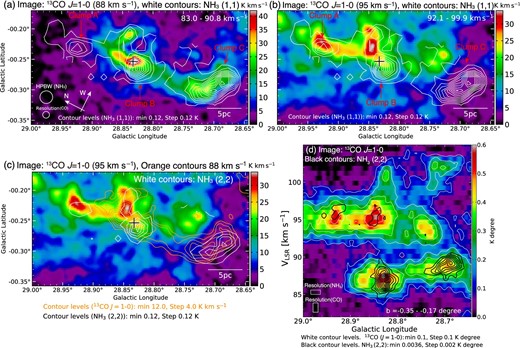
FUGIN 13CO integrated intensity map of two molecular filaments identified by Dewangan, Ojha, and Zinchenko (2017). The integrated velocity range of (a) 83.0–90.8 km s−1 and (b) 92.1–99.9 km s−1, respectively. White contours indicate the NH3(J, K) = (1, 1) peak intensity. The lowest white contour level and intervals are 0.12 K (∼4σ). (c) The integrated intensities of the 88 km s−1 component (orange contours) and 95 km s−1 components (background image). White contours indicate the NH3(J, K) = (2, 2) peak intensity. The cross marks are the same as in figure 2a. (d) The longitude–velocity diagram of 13CO J = 1–0 is shown as white contours. The lowest white contour level and intervals are 0.1 K degree. The black contours present the NH3 (2, 2) intensity of the same integrated latitude range. The lowest black contour level and intervals are 0.0036 K degree and 0.002 K degree, respectively.
5 Summary
The conclusions of our paper are summarized as follows:
We have performed the NH3(J, K) = (1, 1), (2, 2), and (3, 3) survey toward the Galactic infrared bubble N49 (G28.83−0.25) as a part of the KAGONMA project led by the Kagoshima University.
We found three NH3 clumps (A, B, and C) along the molecular filament with radial velocities of ∼96, 87, and 89 km s−1, respectively.
The kinetic temperature derived from NH3(2, 2)/NH3 (1, 1) shows Tkin = 27.0 ± 0.6 K enhanced at Clump B in the eastern edge of the bubble, the position of which coincides with MYSOs associated with the 6.7 GHz methanol maser source. This result shows the dense clump is locally heated by the stellar feedback from the embedded MYSOs.
The NH3 Clump B also exists at the 88 km s−1 and 95 km s−1 molecular filament intersection. Therefore, we suggest that the filament–filament interaction scenario argued by Dewangan, Ojha, and Zinchenko (2017) can explain the NH3 dense gas formation in Clump B.
The NH3 Clumps A and C at the northern and southern sides of the molecular filament exist ∼5–10 pc away from the edge of the bubble traced by the 1.4 GHz radio continuum image. This result suggests that these clumps are likely to occur in spontaneous star formation, and are not affected by the ionization feedback from the N49 bubble.
Acknowledgements
We are grateful to the anonymous referee for carefully reading our manuscript and giving us thoughtful suggestions, which greatly improved this paper. The Nobeyama 45 m radio telescope is operated by the Nobeyama Radio Observatory, a branch of the National Astronomical Observatory of Japan. The authors wish to thank all staff of the Nobeyama Radio Observatory for their assistance in our backup observations. The NH3 backup observations are the result of a number of contributions from people at Kagoshima University, and the authors would like to thank all of them; Dr. Tatsuya Kamezaki, Dr. Gabor Orosz, Dr. Mitsuhiro Matsuo, Mr. Hideo Hamabata, Mr. Tatsuya Baba, Mr. Ikko Hoshihara, Mr. Kohei Mizukubo, Mr. Tatsuya Sera, and Mr. Masahiro Uesugi. M.K. appreciated the curators of the Astronomy Section of Nagoya City Science Museum supporting my research works. The data of the FUGIN project was retrieved from the JVO portal 〈http://jvo.nao.ac.jp/portal/〉 operated by ADC/NAOJ. The data analysis was carried out at the Astronomy Data Center of the National Astronomical Observatory of Japan. The ATLASGAL project is a collaboration between the Max-Planck-Gesellschaft, the European Southern Observatory (ESO) and the Universidad de Chile. It includes projects E-181.C-0885, E-078.F-9040(A), M-079.C-9501(A), M-081.C-9501(A) plus Chilean data. This work is based in part on observations made with the Spitzer Space Telescope, which was operated by the Jet Propulsion Laboratory, California Institute of Technology under a contract with NASA.
