


Abstract
In order to evaluate the impacts made by super-Eddington accretors on their environments precisely, it is essential to guarantee a large enough simulation box and long computational time to avoid any artefacts from numerical settings as much as possible. In this paper, we carry out axisymmetric two-dimensional radiation hydrodynamic simulations around a 10 M⊙ black hole in large simulation boxes and study the large-scale outflow structure and radiation properties of super-Eddington accretion flow for a variety of black hole accretion rates, |${\dot{M}}_{\,\,\rm BH} = (110\!-\!380)L_{\rm Edd}/c^{\,\,2}$| (with LEdd being the Eddington luminosity and c being the speed of light). The Keplerian radius of the inflow material, at which centrifugal force balances with gravitational force, is fixed to 2430 Schwarzschild radii. We find that the mechanical luminosity grows more rapidly than the radiation luminosity with an increase of |${\dot{M}}_{\,\,\rm BH}$|. When seen from a nearly face-on direction, especially, the isotropic mechanical luminosity grows in proportion to |${\dot{M}}_{\,\,\rm BH}^{\,\,2.7}$|, while the total mechanical luminosity is proportional to |${\dot{M}}_{\,\,\rm BH}^{\,\,1.7}$|. The reason for the former is that the higher |${\dot{M}}_{\,\,\rm BH}$| is, the more vertically inflated the disk surface becomes, which makes radiation fields more confined in the region around the rotation axis, thereby strongly accelerating outflowing gas. The outflow is classified into pure outflow and failed outflow, depending on whether the outflowing gas can reach the outer boundary of the simulation box or not. The fraction of the failed outflow decreases with a decrease of |${\dot{M}}_{\,\,\rm BH}$|. We analyze physical quantities along each outflow trajectory, finding that the Bernoulli parameter (Be) is not a good indicator to discriminate between pure and failed outflows, since it is never constant because of continuous acceleration by radiation-pressure force. Pure outflow can arise, even if Be < 0 at the launching point.
1 Introduction
Among diverse black hole objects, super-bright compact sources called ultra-luminous X-ray sources (ULXs) exhibit rather unique observational features; they are bright, with luminosities being over 1039 erg s−1, but they are located at a off-center regions; that is, they are not active galactic nuclei (AGNs; Long et al. 1981; Fabbiano 1989; Soria 2007; Kaaret et al. 2017). Their central engines are still under discussion; promising models include (1) super-Eddington accretion on to a stellar-mass black hole (King et al. 2001; Watarai et al. 2001; Gladstone et al. 2009; Kawashima et al. 2012; Sutton et al. 2013; Motch et al. 2014; Middleton et al. 2015; Kitaki et al. 2017), (2) super-Eddington accretion on to a neutron star (Basko & Sunyaev 1976; Bachetti et al. 2014; Fürst et al. 2016; Kawashima et al. 2016; Israel et al. 2017; Carpano et al. 2018; Mushtukov et al. 2018; Takahashi et al. 2018), and (3) sub-Eddington accretion on to an intermediate-mass black hole (Makishima et al. 2000; Miller et al. 2004; Miyawaki et al. 2009; Strohmayer & Mushotzky 2009). Here, we focus our discussion on the first case.
The super-Eddington accretion flow has two key signatures: it can shine in excess of the Eddington luminosity, and it has powerful outflows due to the increase in radiation force (Ohsuga et al. 2005; Poutanen et al. 2007; Takeuchi et al. 2010). In particular, outflow is crucially important, since it carries mass, momentum, and energy of gas to the surrounding environment and can assert a significant impact there (Regan et al. 2018; Takeo et al. 2020; Botella et al. 2022; Hu et al. 2022).
To understand the nature of super-Eddington accretors, it is essential to solve the interaction between the radiation and the gas; that is, the radiation hydrodynamics (RHD) simulations are necessary (Eggum et al. 1988; Fujita & Okuda 2005; Ohsuga et al. 2005; Narayan et al. 2017; Ogawa et al. 2017; Kitaki et al. 2018, Takeo et al. 2018). Such RHD simulations have been extensively performed in recent times, followed by radiation magnetohydrodynamics (RMHD) simulations (e.g., Ohsuga et al. 2009; Ohsuga & Mineshige 2011; Jiang et al. 2014, 2019). Furthermore, some of the RHD/RMHD simulations are under the general relativistic (GR) formalism (Fragile et al. 2014; McKinney et al. 2014, 2015, 2017; Sa̧dowski et al. 2015; Sa̧dowski & Narayan 2016; Takahashi et al. 2016).
Here, we wish to point out two key issues involved with most of the current RHD/RMHD simulation studies:
Small box size. The size of the computational box is limited due to the restriction from the computer side. This could lead to overestimation of outflow rate (explained later).
Small angular momenta of injected gas. It is thus difficult to investigate the case of the ULXs, in which the injected materials, presumably supplied from the companion star, seem to have relatively large angular momenta.
It will be useful to define the two key radii: (1) the Keplerian radius, rK, at which the centrifugal force balances with the gravitational force for a given specific angular momentum of the injected gas, and (2) the photon trapping radius, rtrap, inside which photon trapping is effective (Begelman 1978; Ohsuga et al. 2005). If we assume a small Keplerian radius, rK < rtrap, injected material accumulates inside the trapping radius, forming a puffed-up region, from which significant outflow emerges. This may lead to overestimation of the outflow rate |$\dot{M}_{\rm outflow}$| (Kitaki et al. 2021, hereafter K21). If we take small computational boxes, moreover, some of the outflow that falls back into the disk after launch (failed outflow) could be mis-classified as a pure outflow that successfully escaped from the system. This will also lead to overestimation of outflow rates.
To avoid such numerical artefacts as much as possible, K21 performed two-dimensional (2D) axisymmetric RHD simulations, assuming (1) a large Keplerian radius, rK = 2430rS, and adopting (2) a large simulation box of a size of rout = 3000rS so that they could elucidate the disk–outflow structure over a wide region across rtrap. Their simulation was, however, restricted to only one parameter-set case. We wish to expand parameter space to get a more general view of super-Eddington outflow. This is the primary aim of the present study.
We perform the same type of axisymmetric 2D-RHD simulations as that of K21 but for a variety of mass accretion rates under realistic simulation settings. The key questions that we address in the present study are two-fold: (Q1) How do the radiation and mechanical luminosities depend on |$\dot{M}_{\,\,\rm BH}$| and viewing angle, and (Q2) how much material is launched from which radii and to which directions? The plan of the present paper is as follows: We explain calculated models and numerical methods in section 2, and present our results of large-scale outflow structure in section 3. There, we emphasize the |$\dot{M}_{\,\,\rm BH}$| dependence of the radiation and outflow properties. We then give discussion in section 4. The main issues to be discussed are the impact on the environments, energy conversion efficiency, connection with the observations of ULXs, and the Bernoulli parameter along the streamline. The final section is devoted to concluding remarks.
2 Calculated models and numerical methods
2.1 Radiation hydrodynamics simulations
In the present study, we consider super-Eddington accretion flow and associated outflow around black hole with mass of 10 M⊙. We inject mass with a certain amount of angular momentum from the outer simulation boundary at a constant rate (more quantitative description will be given later). For calculating radiation flux and pressure tensors, we adopt the flux-limited diffusion approximation (Levermore & Pomraning 1981; Turner & Stone 2001). We do not solve the magnetic fields in the present simulation, and thus adopt the α viscosity prescription (Shakura & Sunyaev 1973). General relativistic effects are taken into account by employing the pseudo-Newtonian potential (Paczyńsky & Wiita 1980).
Basic equations and numerical methods are the same as those in K21 (see also Ohsuga et al. 2005; Kawashima et al. 2009). We solve the axisymmetric 2D radiation hydrodynamics equations in the spherical coordinates (x, y, z) = (rsin θcos φ, rsin θsin φ, rcos θ), where the azimuthal angle φ is set to be constant and the z-axis coincides with the rotation axis. We put a black hole at the origin. In this paper, we distinguish r as the radius in the spherical coordinates and |$R\equiv \sqrt{x^{2}+y^{2}}$| as the radius in the cylindrical coordinates.
We wish to stress that Compton cooling/heating works not only in the optically thin disk atmosphere (in which Tgas > Trad) but also in the optically thick disk (in which Tgas ∼ Trad). To prove this is the case, we numerically checked the heating and cooling timescales at r = 200rS. In the equatorial region, the timescale of viscous heating is comparable to that of Compton cooling, whereas the timescale of bremsstrahlung cooling is longer than the other two by one order of magnitude or more. We wish to note that Tgas ∼ Trad in the disk region does not necessarily mean that the Compton cooling/heating is unimportant, but rather it means that Tgas ∼ Trad is achieved as the result of efficient Compton cooling/heating.
K21 investigated the magnitude of each term on the right-hand side of the gas energy equation (8) and have concluded that the gas is heated by the viscous heating generated in the disk, but it is immediately converted to radiation energy through Compton scattering, resulting in energy transport in the form of advection cooling.
2.2 Initial conditions and calculated models
As was already mentioned, we adopt a large Keplerian radius (rK = 2430rS) and large computational box size rin = 2rS ≤ r ≤ rout = 6000rS (except in one case, described later). We only solve the upper-half domain above the equatorial plane; i.e., 0 ≤ θ ≤ π/2.
Grid points are uniformly distributed in logarithm in the radial direction; ▵log10r = (log10rout − log10rin)/Nr, while it is uniformly distributed in cos θ in the polar direction; ▵cos θ = 1/Nθ, where the numbers of grid points are (Nr, Nθ) = (200, 240) throughout the present study.
Since the main purpose of this study is to investigate the |${\dot{M}}_{\,\,\rm BH}$| dependence of the super-Eddington flow and outflow, we fix the black hole mass and α viscosity parameter, while we vary mass injection rate |$\dot{M}_{\,\,\rm input}$| (see table 1).
Model parameters.
| Parameter | Symbol | Value(s) |
|---|---|---|
| Black hole mass | MBH[M⊙] | 10 |
| Mass injection rate | |${\dot{M}}_{\rm input} [L_{\rm Edd}/c^2]$| | 350, 500, 700, 2000 |
| Viscosity parameter | α | 0.1 |
| Simulation box: inner radius | rin[rS] | 2.0 |
| Simulation box: outer radius* | rout[rS] | 3000 or 6000 |
| Keplerian radius | rK[rS] | 2430 |
Matter is injected continuously at a constant rate of |$\dot{M}_{\rm input}$| through the outer disk boundary at r = rout and 0.49π ≤ θ ≤ 0.5π. We adopted a relatively smaller solid angle, but this does not necessarily mean a higher velocity for a fixed mass injection rate. This is because although we assume the standard disk relations to determine the density and velocity of the injected gas for a given mass injection rate, the in-fall motion of the gas is soon accelerated to approach the free-fall velocity because of small centrifugal force (note rK < rout). The injected gas is assumed to possess a specific angular momentum corresponding to the Keplerian radius of rK = 2430rS (i.e., the initial specific angular momentum is |$\sqrt{GM_{\,\,\rm BH} r_{\rm K}}$|). We thus expect that inflow material first falls towards the center and forms a rotating gaseous ring with a radius of around r ∼ rK, from which the material slowly accretes inward via viscous diffusion process. We assume that matter freely goes out but does not come in through the outer boundary (r = rout, θ = 0 − 0.49π) or the inner boundary (r = rin).
We assume that the density, gas pressure, radial velocity, and radiation energy density are symmetric at the rotation axis, while vθ and vφ are antisymmetric. On the equatorial plane, on the other hand, ρ, p, vr, vφ, and E0 are symmetric, and vθ is antisymmetric. See Ohsuga et al. (2005) for more detailed descriptions regarding the boundary conditions.
3 Results: Large-scale outflow structure
3.1 Overall flow structure
In this paper, we examine the large-scale time-averaged structure of inflow and outflow in a quasi-steady state, unless stated otherwise. We ran the simulation for 0–24500 s. (See figure 12 in appendix 1 for the light curves of some models.) We first show in figure 1 density (upper) and gas temperature (lower) distributions overlaid with the velocity fields for Model-140 (left-hand panels) and Model-380 (right-hand panels), respectively. All the physical quantities (i.e., temperature, velocity, etc.) except for gas mass density are time-averaged with the weight of gas mass density during the interval of t ∼ 23800–24300 s, while gas mass density is simply time-averaged with no weight. Note that Model-140 and Model-380 correspond to the cases with the injection rates of |$\dot{M}_{\,\,\rm inj} = 350$| and 2000 (LEdd/c2), respectively (see table 2).
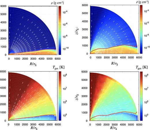
Time-averaged density distributions (upper) and gas temperature distributions (lower) of super-Eddington accretion flow and associated outflow around a black hole in Model-140 (left) and Model-380 (right), respectively. Time average was made during the interval of t ∼ 23800–24300 s. Overlaid are the gas velocity vectors, the lengths of which are proportional to the logarithm of the absolute velocity. The red solid line represents the disk surface, which is defined as the loci where the radiation force balances the gravitational force.
After the simulation starts, the gas injected from the outer boundary into an initially empty zone first falls and accumulates around the Keplerian radius, rK = 2430rS, since the centrifugal force and the gravitational force balance there. Soon after the transient initial phase, accumulated matter spreads outward and inward in the radial direction via viscous diffusion process, forming an accretion disk extending down to the innermost zone (t ≲ 23800 s). The newly injected matter collides with the disk matter so that a high-density region appears at ∼(2400–6000) rS (well outside the Keplerian radius) in figure 1. In a sufficiently long time (on the order of the viscous timescale, t ≳ 23800 s; Ohsuga et al. 2005), quasi-steady, inflow–outflow structure is established (see figure 1).
In figure 1 we also indicate the disk surface by the red solid line. The disk surface was defined in the same way as in K21, with the loci where radiation force balances the gravity in radial direction, χF0, r/c = ρGMBH/(r − rS)2. As in K21, the disks are smoothly connected up to the outer boundary, and there is no puffed-up structure as seen in the previous RHD simulations (see table 1 in K21).
We think that rK < rtrap is the only reason to produce a puffed-up structure, for the following reason. When we compare Kitaki et al. (2018) and K21 in which the same code was used and |$\dot{M}_{\,\,\rm BH}$| is not much different, only the former (with rK < rtrap) shows a puffed-up structure, while the latter (with rK > rtrap) does not. The outflow rate in the former is 10 times larger than that of the latter. These indicate that the high mass outflow rates obtained in the previous studies could be caused by setting a small initial angular momentum (see section 1 of K21).
We understand from the velocity fields in figure 1 that gas is stripped off from the disk surface to form outflow. We also plot the velocity fields of gas by the white vectors in figure 1. Near the rotation axis, especially, we see a cone-shaped funnel filled with high-velocity (≳0.3 c), low-density, and high-temperature Tgas ≳ 108 K plasmas surrounded by an outflow region of modest velocity (∼ 0.05–0.1c) and modest temperatures, Tgas ∼ 106 − 7 K. This velocity and temperature feature is seen in both Model-140 and Model-380. In both accretion disks, we can see the circular motions (see K21 for detailed analysis).
3.2 Mass inflow rate and mass outflow rate
Figure 2 illustrates the absolute values of the various mass flow rates as functions of radius, r. We here omit the mass inflow rate in the outflow, since it turns out to be practically zero.
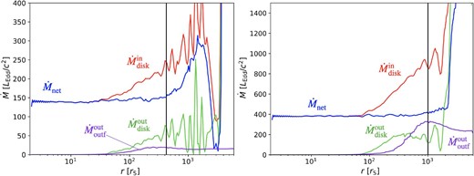
Time-averaged radial profiles of inflow/outflow rate of Model-140 (left-hand panel) and Model-380 (right-hand panel) during the interval of t ∼ 23800–24300 s. Shown is the mass inflow rate within the disk, |$\dot{M}_{\,\,\rm disk}^{\rm \,\,in}$| (red line), the mass outflow rate within the disk, |$\dot{M}_{\,\,\rm disk}^{\,\,\rm out}$| (green line), the net flow rate, |$\dot{M}_{\rm net}$| (blue line), and the mass outflow rate in the outflow region (above the disk surface), |$\dot{M}_{\,\,\rm outf}^{\,\,\rm out}$| (purple line), respectively. The net flow rate is nearly constant inside the quasi-steady radius, rqss ∼ 400rS at Model-140 and ∼1000rS at Model-380, which is indicated by the vertical black line.
Let us first focus on the case of Model-380 (see the right-hand panel of figure 2). The blue line, which represents the net accretion rate, provides important information to judge to what extent a quasi-steady state is achieved. We see that it is approximately constant in the range of r = (2–1000)rS; that is, the quasi-steady radius (inside which a quasi-steady state is realized) is rqss ∼ 1000rS.
We notice that the mass outflow rate is negligibly small not only in the far outer region but also in the innermost region (see also K21). We estimate the radius, |$R_{\rm pure}^{\rm in }$| (=Rinflow in K21), inside which outflow is negligible, by the intersection of the two lines: |$\dot{M}_{\,\,\rm disk}^{\,\,\rm in}(r)$| and |$\dot{M}_{\,\,\rm net}(r)$|, finding |$R_{\rm pure}^{\rm in} \sim 40 r_{\rm S}$|. The mass inflow rate in the disk region and the outflow rate in the outer region averaged over the range of r = (2–30)rS are |$\dot{M}_{\,\,\rm BH}\equiv \langle |\dot{M}_{\,\,\rm disk}^{\,\,\rm in}|\rangle =380L_{\rm Edd}/c^{2}$| and |$\langle \dot{M}_{\rm outf}^{\rm out}\rangle =0.13L_{\rm Edd}/c^{2}$|, respectively (see also table 2).
Radiation and outflow properties.*
| Quantity | Model-110 | Model-130 | Model-140 | Model-180 | Model-380 | |
|---|---|---|---|---|---|---|
| BH accretion rate | |$\dot{M}_{\rm BH}$| [LEdd/c2] | ∼110 | ∼130 | ∼140 | ∼180 | ∼380 |
| Mass injection rate | |$\dot{M}_{\rm inj}$| [LEdd/c2] | 350 | 500 | 700 | 700 | 2000 |
| Outflow rate at rout | |$\dot{M}_{\rm outflow}$| [LEdd/c2] | ∼10 | ∼13 | ∼16 | ∼24 | ∼230 |
| Failed outflow rate at rout | |$\dot{M}_{\rm failed}$| [LEdd/c2] | 0 | ∼4 | ∼8 | ∼15 | ∼100 |
| Quasi steady-state radius | rqss [rS] | ∼500 | ∼400 | ∼400 | ∼600 | ∼1000 |
| Pure outflow: inner radius | |$R_{\rm pure}^{\rm in}$| [rS] | ∼40 | ∼40 | ∼40 | ∼40 | ∼40 |
| Pure outflow: outer radius | |$R_{\rm pure}^{\rm out}$| [rS] | ∼170 | ∼110 | ∼130 | ∼180 | ∼480 |
| Failed outflow: outer radius | |$R_{\rm failed}^{\rm out}$| [rS] | ∼170 | ∼180 | ∼210 | ∼210 | ∼820 |
| Photon trapping radius | Rtrap [rS] | ∼300 | ∼330 | ∼350 | ∼450 | ∼1100 |
| X-ray luminosity | LX [LEdd] | ∼2.0 | ∼2.1 | ∼2.3 | ∼2.4 | ∼2.7 |
| Mechanical luminosity | Lmech [LEdd] | ∼0.07 | ∼0.09 | ∼0.11 | ∼0.16 | ∼0.61 |
| Isotropic X-ray luminosity | |$L_{\rm X}^{\rm ISO} (\theta )$| [LEdd] | 2.0–4.0 | 2.3–4.4 | 2.4–4.8 | 2.3–4.6 | 2.1–11 |
| Isotropic mechanical luminosity | |$L_{\rm mech}^{\rm ISO}(\theta )$| [LEdd] | 0.04–0.18 | 0.02–0.35 | 0.03–0.60 | 0.04–1.4 | 1.0–8.0 |
| Luminosity ratio | |$L_{\rm mech}/L_{\rm X}^{\rm ISO}(\theta )$| | 0.02–0.04 | 0.02–0.04 | 0.02–0.05 | 0.04–0.07 | 0.06–0.29 |
Note again that the results of Model-180 are taken from K21. In the calculations of isotropic luminosities (see the last three rows), we take an angular range of 0° < θ < θsurf.
We are now ready to examine where outflow emerges by the examination of the lines in the middle region (80–1000) rS. The outflow rate above the disk surface, |$\dot{M}_{\,\,\rm outf}^{\,\,\rm out}$| (indicated by the purple line in figure 2), increases with increasing radius, reaches its maximum value of 320LEdd/c2 at |$r=1000r_{\rm S} (\equiv r_{\rm failed}^{\rm out})$|, and then decreases beyond that. This position, |$r_{\rm failed}^{\rm out}$| (=rlau in K21), corresponds to the outermost launching position of the outflows. The fact that |$\dot{M}_{\,\,\rm outf}^{\,\,\rm out}$| decreases beyond |$r_{\rm failed}^{\rm out}$| means that some of the outflow materials fall back on to the disk surface (see K21). Therefore, this decrement in the |$\dot{M}_{\,\,\rm outf}^{\,\,\rm out}$| curve gives the failed outflow rate.
In the further outer region, r ≳ 3000rs, |$\dot{M}_{\,\,\rm outf}^{\,\,\rm out}$| is nearly constant. The space-averaged (genuine) outflow rate at r = (4000–6000)rS is |$\dot{M}_{\,\,\rm outflow}\equiv \langle \dot{M}_{\rm outf}^{\rm out}\rangle \sim 230L_{\rm Edd}/c^{2}$|. The total amount of failed outflow is |$\dot{M}_{\rm failed}= 100 L_{\rm Edd}/c^2$|.
Similar analyses can be repeated for Model-140 (see the left-hand panel of figure 2). The results of outflow rate evaluations are summarized in table 2, including those models not plotted in figure 2.
Note that the mass accretion rate on to a black hole (|${\dot{M}}_{\,\,\rm BH}$|) is determined by mass flow rate at r = rqss, and not by the mass injection rate at the outer boundary. It thus happens that different accretion rates may appear for the same mass injection rate, as in the case of Model-140 and Model-180. We should also note that since high–low transitions are observed in Model-110, we time-averaged over 200 s solely during the super-Eddington state to calculate quantities listed in table 2.
3.3 Outflow streamlines
The streamline analysis is useful to understand the outflow path and the evolution of physical quantities of the outflowing gas after being launched. The upper panel of figure 3 displays a sequence of streamlines overlaid on the temperature contours, while the lower panel is the magnified view of the central region of the upper panel. We understand in this figure that the outflow emerges from the disk surface inside the white circle of the radius, r ∼ 1000rS, where |$\dot{M}_{\,\,\rm outf}^{\,\,\rm out}$| reaches its maximum (see figure 3). We here define the farthest launching radius |$R_{\rm failed}^{\rm out}$| (= Rlau in K21) where the white line crosses the red line; that is |$R_{\rm failed}^{\rm out} = r_{\rm failed}^{\rm out}\sin {\theta _{\rm surf}}\sim 1000\sin {\left(0.96\right)} r_{\rm S} \sim 820r_{\rm S}$|.
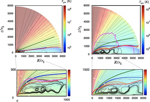
Sequences of streamlines overlaid on the gas temperature distributions for Model-140 (left-hand panel) and Model-380 (right-hand panel), respectively. The upper panels are the large-scale view, while the lower ones are the magnification of the central region. In each panel we pick up several streamlines and color them: The green line and the orange line indicate a sample streamline in the pure outflow and the same in the failed outflow, respectively, while the blue line shows an interface separating pure and failed outflow regions. The red line represents the disk surface, and the white line indicates the radius (r), at which the cumulative outflow rate reaches its maximum.
The region between the blue and red lines in figure 3 indicate the region of the failed outflow; that is, the outflow which leaves the disk surface at small radii but eventually comes back to the disk at large radii (see also K21). The farthest launching radius of the pure outflow (which can reach the outer boundary of the computational box) is given by |$R_{\rm pure}^{\rm out}=r_{\rm pure}^{\rm out} \sin {\theta _{\rm surf}}\sim\,\,650 \sin {\left(0.72\right)} r_{\rm S} \sim 480r_{\rm S}$| (|$= R_{\rm lau}^{\infty }$| in K21). Here, we define the inner edge of failed outflow, |$R_{\rm failed}^{\rm in}$|. Note |$R_{\rm pure}^{\rm out} = R_{\rm failed}^{\rm in}$| by definition and this radius is the inner intersection of the blue and red lines in figure 3.
In fact, we see in figure 3 that the outflow launching from the disk surface at |$R_{\rm pure}^{\rm out}\le R \le R_{\rm failed}^{\rm out}$| does return to the disk surface at larger radii.
As seen in figure 3, the outflow launching region can rigorously be identified through the streamline analysis. As a result, the disk surface can be divided into several regions: (1) the innermost region, where outflow rate is negligible, (2) the inner region, where pure outflow emerges, (3) the middle region, where failed outflow emerges, and (4) the outer region, where again outflow rate is negligible. Note that region (3) disappears at very low accretion rate (i.e., Model-110). These results are consistent with K21.
We notice that the radii of the inner boundaries of the outflow launching regions (i.e., |$R_{\,\,\rm pure}^{\,\,\rm out}$| and |$R_{\,\,\rm failed}^{\,\,\rm out}$|) more steeply increase with increase of |$\dot{M}_{\,\,\rm BH}$| than the trapping radius. This result does not precisely agree with the estimation by the (semi-)analytical model (e.g., Shakura & Sunyaev 1973; Fukue 2004) which shows |$R_{\,\,\rm pure}^{\,\,\rm out} \sim \dot{M}_{\,\,\rm BH}/(L_{\rm Edd}/c^2) r_{\rm S}$| (although that those authors did not distinguish between pure and failed outflows; see also K21).
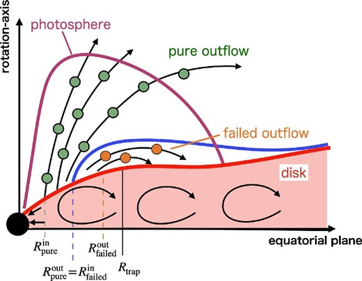
Schematic view of the outflow structure of super-Eddington accretion flow. (This figure is basically the same as that shown in K21 except for minor modifications.) The pink and blue lines represent the photosphere and the interface between the pure outflow region and failed outflow region, respectively. The outflow structure is divided into four regions: (1) the innermost region with negligible outflow (|$R\le R_{\rm pure}^{\rm in}$|), (2) the inner region producing pure outflow (|$R_{\rm pure}^{\rm in} \le R \le R_{\rm pure}^{\rm out}$|), (3) the middle region producing failed outflow (|$R_{\rm pure}^{\rm out} \le R \le R_{\rm failed}^{\rm out}$|), and (4) the outer region with negligible outflow, respectively (see K21).
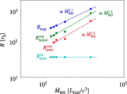
Launching sites of pure and failed outflows as functions of |$\dot{M}_{\,\,\rm BH}$|. The cyan, red, green, and blue lines respectively represent |$R_{\,\,\rm pure}^{\,\,\rm in}$|, |$R_{\,\,\rm pure}^{\,\,\rm out}$|, |$R_{\rm failed}^{\rm out}$|, and Rtrap. Note that we use the data of K21 to plot in this profile.
Numerically, our estimations agree reasonably well with theirs at higher accretion rates, e.g., |${\dot{M}}_{\,\,\rm BH} \sim\,\,10^2 L_{\rm Edd}/c^2$|, while ours are much less at lower accretion rates, as is shown by the steeper power-law dependence (|$\propto {\dot{M}_{\,\,\rm BH}}^{1.4}$|) in figure 5. In other words, outflow emergence region (between |$R_{\,\,\rm pure}^{\,\,\rm in}$| and |$R_{\rm failed}^{\rm out}$|) shrinks with a decrease of the accretion rate more rapidly than the simple estimations.
3.4 Radiation and mechanical luminosities
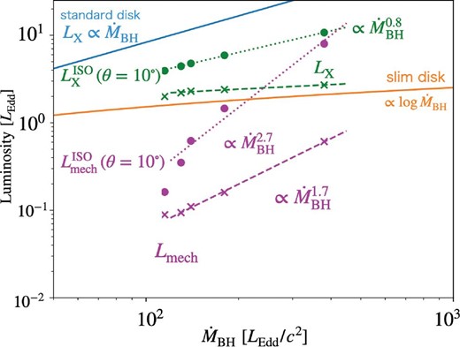
X-ray and mechanical luminosities as functions of |$\dot{M}_{\,\,\rm BH}$|. The dashed line and the dotted line represent luminosity and isotropic luminosity, respectively. For calculation for isotropic luminosity, a viewing angle of θ = 10° is assumed. The green, magenta, blue, and yellow lines represent the radiation and mechanical luminosities calculated by our analyses, the radiation luminosity predicted by the standard disk model, and the same predicted by the slim disk model, respectively.
There are several noteworthy features found in this figure. First, we focus on the radiation luminosity (the green dashed and dotted lines). The radiation luminosity (dashed line) shows the |$\dot{M}_{\,\,\rm BH}$| dependence similar to the slim disk model (the orange solid line). By contrast, the isotropic radiation luminosity (dashed line) depends on |$\dot{M}_{\,\,\rm BH}$| more sensitively than the (total) luminosity. For a nearly face-on observer (with θ ∼ 10°) we estimate |$L_{\rm X}^{\rm ISO} (10^\circ ) \propto \dot{M}_{\,\,\rm BH}^{\,\,0.8}$|. Why do the isotropic radiation luminosity and radiation luminosity vary differently? This is because of the fact that the radiation energy release is not isotropic, and that the higher the accretion rate is, the more focused the radiation flux becomes towards the rotation axis.
Next, we consider the behavior of mechanical luminosity (magenta dashed and dotted lines) with respect to |$\dot{M}_{\,\,\rm BH}$|. Figure 6 shows that mechanical luminosity is more sensitive to |$\dot{M}_{\,\,\rm BH}$| than X-ray luminosity. In particular, isotropic mechanical luminosity is found to follow the power-law relation, as |$\propto \dot{M}_{\,\,\rm BH}^{\,\,2.7}$|. We wish to note that the fittings are performed with the exclusion of Model-110. This is because isotropic mechanical luminosity drops sharply there, as the luminosity approaches the Eddington luminosity. (Note that radiation-pressure driven outflow no longer arises at the Eddington luminosity, since then the radiation force is equal to the gravitational force.)
We emphasize again the steeper |$\dot{M}_{\,\,\rm BH}$| dependence of mechanical luminosities than radiation luminosities. The difference between them is more enhanced, when we consider isotropic luminosities. For a nearly face-on observer (with θ ∼ 10°), especially, |$L_{\rm mech}^{\rm ISO}(10^\circ )$| becomes comparable to |$L_{\rm X}^{\rm ISO}(10^\circ )$| at |$\dot{M}_{\,\,\rm BH}\sim 400 L_{\rm Edd}/c^2$| (or at luminosities of ∼10LEdd). Such enhanced impact by massive outflow may explain the existence of the anisotropic (elongated) shape of the ULX bubble. However, we should keep in mind that (unlike the isotropic radiation luminosities) the isotropic mechanical luminosities are not easy to measure observationally, since the impact of the outflow tends to be more or less circularized within a bubble. We would do better to discuss in terms of isotropic radiation luminosities and total mechanical luminosities (see also discussion in subsection 4.3).
3.5 Why is isotropic mechanical luminosity so sensitive to accretion rate?
Why does |$L_{\rm mech}^{\rm ISO}$| exhibit an extremely large |$\dot{M}_{\,\,\rm BH}$| dependence? Since mechanical luminosity depends on density and radial velocity, such a rapid growth should be a large increase of either of ρ or vr, or both. To explore the reason, we plot in the left-hand panel of figure 7 the angular (θ) distributions of density and radial velocity at r = 5000rS for various models. The result is that density increases with increasing θ for all models, while radial velocity instead decreases. (As for the angular profiles of the gas density at other radii, see appendix 2.) In the polar direction, radial velocity does not differ between the models, but density differs significantly. This gives direct evidence that the rapid growth of the mechanical luminosity is due to the rapid increase in density, not in velocity.
![[Left-hand panel] Angular (θ) distributions of the density (solid line) and radial velocity (dashed/dotted line) at r = 5000rS for various models: Model-380 (green), Model-180 (blue), Model-140 (pink), and Model-130 (orange), respectively. The dashed and dotted lines are outflow and inflow, respectively. [Right-hand panel] Same as the left-hand panel but for the distribution of the mass flux [multiplied by r2 × sin (θ)]. The solid and dashed lines are outflow and inflow, respectively.](https://oup.silverchair-cdn.com/oup/backfile/Content_public/Journal/pasj/74/6/10.1093_pasj_psac076/3/m_psac076fig7.jpeg?Expires=1749234176&Signature=nnfCogVERz9O2Kgty6u6a-ukdwGGuTIrnq0qRY0M3Wb6I2lyD7aKDL1En62cZKskKOtsTqYm-7Ucp1BNFk7BrqiFi-TlszjO~kE~A6lMeDp94Lm-5g6Fc~XJFcJfAAYmebCmhHyAxr3bRnoWinP4PxAHeyj62qTyOs4unytnjeN0lB5rYbXqNe0USgclEINp3BZTn79bk5aqsDz-ZBrGzaQeae0W3togDW1NxLZJMi7LgAC3kyDSZ96K~oGhQPluCSmMH0t4EFZUv0k3De3Q8FJ21JA14JjsnDglmxQH0~04WpA~KgdXAR3CycSHBmDSQFaEZOOGyjadUQpPBlWO1g__&Key-Pair-Id=APKAIE5G5CRDK6RD3PGA)
[Left-hand panel] Angular (θ) distributions of the density (solid line) and radial velocity (dashed/dotted line) at r = 5000rS for various models: Model-380 (green), Model-180 (blue), Model-140 (pink), and Model-130 (orange), respectively. The dashed and dotted lines are outflow and inflow, respectively. [Right-hand panel] Same as the left-hand panel but for the distribution of the mass flux [multiplied by r2 × sin (θ)]. The solid and dashed lines are outflow and inflow, respectively.
We also plot the mass flux multiplied by r2 × sin θ (right-hand panel of figure 7) at r = 5000rS. This shows that more mass flux goes more preferentially into the intermediate direction than in the polar direction. We also see that the higher accretion rate is, the greater the mass flux profile becomes (except at very small θ values).
If we use the relationship |$L_{\rm mech}^{\rm ISO}\propto \rho \times v_r^3$|, and if we insert the values at θ = 10°, we estimate |$L_{\rm mech}^{\rm ISO} \propto \dot{M}_{\,\,\rm BH}^{\,\,2.7}$|, in reasonable agreement with the result in figure 6. If we instead adopt the averaged values, we obtain |$\rho ^{\rm ave} \times \left(v_r^{\rm ave} \right)^{3} \propto \dot{M}_{\,\,\rm BH}^{\,\,1.1}$|, which does not agree as much.
Why does the density increase more rapidly towards the polar direction, when mass accretion rates are high? To elucidate the reason for this, we plot the distributions of the radial component of the radiation force per unit mass, χF0,r/cρ, for Model-140 and Model-380 in the left- and right-hand panels, respectively, of figure 9. We there find that the region of strong radiation force per unit mass is more concentrated towards the polar direction, when the mass accretion rate is high (see the right-hand panel). This seems to be caused by the vertically inflated disk surface, which makes the radiation field more confined in the region around the rotation-axis, thereby accelerating outflowing gas more strongly.
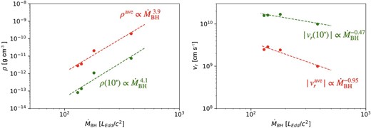
|$\dot{M}_{\,\,\rm BH}$| dependence of ρ (left) and vr (right) at 5000rS. The red and green lines represent the average value in the flat profile (θ = 30°–60° in Model-380) in figure 9, right-hand panel, and the value in the polar direction (θ = 10°), respectively.
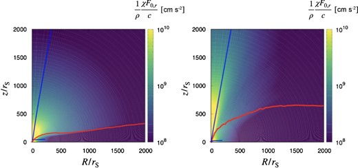
Two-dimensional distribution of the radiation force per unit mass (i.e., |$\frac{1}{\rho }\frac{\chi F_{0,r}}{c}$|) for Model-140 (left-hand panel) and Model-380 (right-hand panel), respectively. The red and blue lines represent the disk surface and the straight line with θ = 10°, respectively. We see a more collimated high-acceleration region (indicated by the yellow color) in the right-hand panel. This seems to be created due to the self-obscuration, since we see in the right-hand panel a more vertically inflated disk surface (see the red line, which stands for the disk surface).
4 Discussion
4.1 Impact on the environments
It has been suggested that the super-Eddington accretion flow will give large impacts on its environments through powerful outflows. It is thus crucial to quantify the magnitudes of the impacts from the super-Eddington accretors to understand the AGN feedback effects properly (King & Pounds 2003; Botella et al. 2022).
Figure 10 shows the polar angle (θ) profile of the energy fluxes in the laboratory frame (multiplied by r2) measured at r = 5000rS for all models. The solid (dashed) lines represent the radiation (mechanical) energy fluxes.
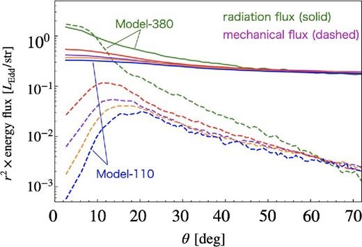
Polar angle (θ) dependences of the radiation (solid) and mechanical (dashed) energy fluxes measured at r = 5000rS for Model-380 (green), Model-180 (red), Model-140 (purple), Model-130 (orange), and Model-110 (blue). Note that the disk surface is located at θ = 72° in the case of Model-380.
Let us first discuss the properties of the radiation energy flux. We see that the radiation energy flux shows a more or less flat profile, but we notice some distinction at small θ values. That is, the radiation energy flux steadily grows towards the rotation axis (θ = 0) in Model-380, whereas it is flatter in Model-110.
We numerically checked the θ dependence of each term in equation (22), finding that the rapid increase in the energy flux towards the rotation axis, which occurs only when accretion rates are large, is due to the increase of the second and third terms in equation (22). We may thus conclude that the distinct shapes of the lines of figure 10 are due to the enhanced advection of the radiation energy within high |$\dot{M}_{\,\,\rm BH}$| outflow propagating towards the face-on direction.
By contrast, the mechanical energy flux displayed in figure 10 exhibits somewhat different behavior; it tends to increase with decrease of θ, reaches its maximum at around θ ∼10°–20°, and then rapidly decreases towards the rotation axis (except in Model-380). As seen in figure 7, the density curves show similar angular dependence in all models. The radial velocity profiles, in contrast, exhibit distinct behavior; that is, the radial velocity in Model-380 rapidly increases toward the polar direction, whereas that in the other models only gradually increases. Because of such somewhat different velocity profiles with the different mass accretion rates, the impact of the mechanical energy flux on the surroundings becomes more anisotropic, as the accretion rate increases. To summarize, the angular dependence of the energy flux exhibits distinct trends, depending on the accretion rate.
4.2 The energy conversion
Energy conversion.
| Model | |$\dot{M}_{\,\,\rm BH} [L_{\rm Edd}/c^2]$| | |$\dot{M}_{\,\,\rm outflow} [L_{\rm Edd}/c^2]$| | β* | βin | βout† |
|---|---|---|---|---|---|
| Model-110 | ∼110 | ∼10 | 0.11 | 0.92 | 0.08 |
| Model-130 | ∼130 | ∼13 | 0.10 | 0.91 | 0.09 |
| Model-140 | ∼140 | ∼15 | 0.11 | 0.90 | 0.10 |
| Model-180 | ∼180 | ∼24 | 0.14 | 0.88 | 0.12 |
| Model-380 | ∼380 | ∼230 | 0.61 | 0.62 | 0.38 |
In parallel with the present work, Hu et al. (2022) performed series of large-scale and long-term simulations of super-Eddington accretion flows, adopting various boundary conditions under the optically thick limit, and obtained a larger β value; e.g., β ∼ 32.9 for |${\dot{M}}_{\,\,\rm BH}\sim 311 L_{\rm Edd}/c^2$|. In addition, they showed a gentler |${\dot{M}}_{\,\,\rm BH}$|-dependence of the momentum flux, |${\dot{P}}_{\rm mom}$|; that is, roughly |${\dot{P}}_{\rm mom}\propto {\dot{M}}^{1}$|, while our results show |${\dot{P}}_{\rm mom}\propto {\dot{M}}^{2}$|. Numerically, their value is about six times larger at |${\dot{M}}_{\,\,\rm BH}\sim 100 L_{\rm Edd}/c^2$|, and about twice at |${\dot{M}}_{\,\,\rm BH}\sim 380 L_{\rm Edd}/c^2$|. Hu et al. (2022) claimed that the reasons for the differences from K21, in which the same method is employed as the present work, are due to (1) the assumption of equatorial plane symmetry and (2) the large alpha parameter in our calculations. The cause of the difference will be studied in future work. We here point out that the outflow region is not entirely optically thick (for absorption) when the mass accretion rate is low, so the equality between the radiation energy and gas energy density may not always hold.
4.3 Connection with observations of ULXs
We next discuss observational implications of our model. A good target is the ULXs, since they are occasionally associated with optical nebula and/or radio bubbles (e.g., Kaaret et al. 2004), and since these nebulae are thought to originate from the outflow in super-Eddington accretion flow (Hashizume et al. 2015). The X-ray luminosity via direct observations of the central objects can be evaluated by us, while the mechanical luminosity can be estimated by observing optical radiation from the ULX bubble. As K21 have already pointed out, the ratio of |$L_{\rm mech}/L_{\rm X}^{\rm ISO}(\theta )$| should be a good indicator to discriminate whether the central object of a ULX is a black hole or a neutron star. In table 2 we summarize the ratios estimated based on our simulations. In Model-380, for example, the ratio ranges between 0.06 and 0.29, depending on the angle, θ. We find somewhat smaller values in other models, but at least we may conclude that these values are consistent with the observations, which is 0.04–0.14 for Holmberg II X-1 (Abolmasov et al. 2007).
4.4 Bernoulli parameter along streamlines
In order to investigate what factor is responsible for separating failed outflow and pure outflow, we calculate the energy distribution along the respective streamlines of pure and failed outflows. The top panel of figure 11 shows energy distribution along the two representative streamlines which are shown in figure 3 as the green and orange lines; the former corresponds to the pure outflow (left-hand panel), while the latter to the failed outflow (right-hand panel). The red line (Egrav), blue line (Erad), and green line (Emech) in each panel represent the gravitational energy [GM/(r − rS)], the radiation energy (E0/ρ), and the mechanical energy (v2/2), respectively. In both flows, the gravitational energy dominates over others at the launching point. In the left-hand panel, however, the kinetic energy eventually exceeds the gravitational energy during the course of outflow propagation, thereby producing pure outflow. In the right-hand panel, by contrast, the kinetic energy is entirely less than the gravitational energy, such that the failed outflow should appear. Only when outflowing gas travels in the region with large Erad for a certain time can it become pure outflow.
![[Top] Energy distribution along one streamline in the pure outflow (left-hand panel) and another in the failed outflow (right-hand panel). The red, blue, and green lines represent the gravitational energy, the radiation energy, and the mechanical energy, respectively. The magenta dashed line indicates the position of the photosphere. [Middle] Same as the top panel but for the specific Bernoulli parameter of the gas + radiation component (solid line) and of the gas component only (dashed line). [Bottom] Same as the top panel but for the polar angles of the velocity vector (black), the total force vector (green), the radiation force vector (blue), and the centrifugal force vector (red), respectively.](https://oup.silverchair-cdn.com/oup/backfile/Content_public/Journal/pasj/74/6/10.1093_pasj_psac076/3/m_psac076fig11.jpeg?Expires=1749234176&Signature=hma7bfkP9ViuuwGfHHbSQzeuiffu4PiJWZUn3lgzIv-8k8ujaIX2ZM4x-KASvcU01QJHNNZ~g22UDdZvmhbC4L~KXFaaex8cHkfUimAFb3h2ukZ-02cEBr3uR2p~iMgE3yke5UdDnlqrZDhqosNY2N~rihvDWcaPGBhPxBHjMLL9DP~kvcByD9oOtVqNMX~ZXJO9hsP9fWli37aImGBICrI9UopUWiCM2Mx0D56clguh8OqZRCYr26Tubtpqwy8ksTwhbrC08InEscXncpeEJMWOSu0WJO4R-CrMP4scf8Q9cmUwP42zYRykTB~q-832DkPGBeK7q0C4VsU0gqiW3Q__&Key-Pair-Id=APKAIE5G5CRDK6RD3PGA)
[Top] Energy distribution along one streamline in the pure outflow (left-hand panel) and another in the failed outflow (right-hand panel). The red, blue, and green lines represent the gravitational energy, the radiation energy, and the mechanical energy, respectively. The magenta dashed line indicates the position of the photosphere. [Middle] Same as the top panel but for the specific Bernoulli parameter of the gas + radiation component (solid line) and of the gas component only (dashed line). [Bottom] Same as the top panel but for the polar angles of the velocity vector (black), the total force vector (green), the radiation force vector (blue), and the centrifugal force vector (red), respectively.
The middle panel of figure 11 show the distribution of the specific Bernoulli parameter of gas component only (dotted line) and the total one (solid line), respectively. We first notice that they are not constant but increase as the outflow propagates, since the gas is continuously accelerated by the radiation force. We also find that the specific Bernoulli parameters are negative at the launching points in both flows shown here. A difference is found in that the Bernoulli parameter of gas can only eventually become positive at around the position of the photosphere in pure outflow, while it never becomes positive in failed outflow. Thus, we conclude that the condition for pure outflow is that the Bernoulli parameter of gas can only become positive before reaching the photosphere. To summarize, our simulations demonstrate that pure outflow emerges, even if Be < 0 near the launching point.
Finally, we examine the bending of the streamline of pure and failed outflows. The bottom panel of figure 11 show the directions of some representative vector quantities along the streamline of pure (left-hand panel) and failed (right-hand panel) outflows as functions of r: the velocity (dotted line), the total force (green solid line), the radiation force (blue solid line), and the centrifugal force (red solid line). Here, by the centrifugal force we mean the combination of the second and third term on the right-hand side of equation (3) and the second term on the right-hand side of equation (4), and by the total force we mean the sum of the radiation force, centrifugal force, and gravitational force. Note that the gas pressure force is negligible.
We see in this figure that the radiation force is mainly upward (with small angles) at the launching point, whereas the centrifugal force is in the R-direction (θ = 90°). Gas is thus initially accelerated in the intermediate direction (θ ∼ 40°) in both cases of pure and failed outflow. Within the pure outflow (see the lower left-hand panel), total force, radiation force, and velocity vectors tend to go in the same direction (with ∼70°) and eventually all the angles coincide with each other. This means that gas dynamics is governed by radiation. No such converging behavior is observed in the failed outflow (see the lower right-hand panel). Since gravitational energy does always exceed the radiation energy, the angle of the velocity vector steadily increases and eventually falls down on to the disk surface.
4.5 The transition in the thermal instability
First of all, we wish to point that the transitions between the super-Eddington and sub-Eddington states (in our Model-110) and the transition to the super-Eddington state shown by Inayoshi et al. (2016) are caused by entirely distinct mechanisms. Inayoshi et al. (2016) considered a region far away from the black hole accretion disk (slightly inside the Bondi radius). In their work, H ii gas in the central region, ionized by UV radiation, pushes the outer H i gas by gas pressure gradient forces. If the mass density of the interstellar gas is high enough, the gravity exceeds the gas pressure gradient force and the gas cannot be prevented from falling. Thus, the H i gas accretes at the supercritical rate.
On the other hand, we focus on the accretion disk much closer to the black hole. The cause of the transition appearing in our Model-110 is the thermal instability of the disk. The heating (cooling) rate exceeds the cooling (heating) rate, causing a runaway temperature increase (decrease), leading to the significant change in the mass accretion rate. According to the disk instability theory [see, e.g., chapter 10 of Kato et al. (2008)], a thermal instability occurs outside the trapping radius in the case that the dynamical viscosity is proportional to the total pressure.
In models other than Model-110, no such instabilities are observed, probably because the spatial extent of the unstable region is limited between the trapping radius and the quasi-steady radius and both radii are closer to each other; that is, rqss/rtrap ∼ 0.9–1.3 in other models (note rqss/rtrap ∼ 1.7 in Model-110; see table 2). As a consequence, a thermal instability, even if it may occur locally, cannot propagate widely to produce global, coherent state transitions. If we could increase the trapping radius, we would be able to obtain state transitions, but such a study is beyond the scope of the present paper and is left as future work.
5 Concluding remarks
In the present study, we perform extensive radiation-hydrodynamics simulations for a variety of mass injection (and mass accretion) rates to see how the properties of radiation and outflow depend on the input parameter. The specific questions that we have in mind are two-fold: (Q1) How do the radiation and mechanical luminosities depend on |$\dot{M}_{\,\,\rm BH}$| and inclination angle, and (Q2) how much material is launched from which radii and in which directions?
In order to avoid numerical artefacts as much as possible and to evaluate the impacts from super-Eddington accretors precisely, we set a relatively large calculation box with box size of 6000rS (or 3000rS) and assume relatively large Keplerian radii (2430rS). We have the following results, some of which were unexpected before the present study.
We find that the mechanical luminosity grows more rapidly than the radiation luminosity with an increase of |${\dot{M}}_{\,\,\rm BH}$|.
Since the isotropic mechanical luminosity (|$\propto {\dot{M}}_{\,\,\rm BH}^{\,\,2.7}$|) grows much faster than the isotropic radiation luminosity (|$\propto {\dot{M}}_{\,\,\rm BH}^{\,\,0.8}$|), the ratio, |$L_{\rm mech}/L_{\rm X}^{\rm ISO}$|, steadily increases as the accretion rate increases. They could be comparable (and are ∼10LEdd) for θ = 10° at the accretion rate of |${\dot{M}_{\,\,\rm BH}} \sim 400 L_{\rm Edd}/c^2$|.
We examined which factor is essential to produce such a rapid growth with accretion rate, finding that it seems to be caused by the vertically inflated disk surface, which makes the radiation field more confined in the region around the rotation axis, thereby accelerating the outflowing gas more strongly.
There are two kinds of outflow: pure outflow and failed outflow. We find that the fraction of the failed outflow decreases as the accretion rate decreases, and that no obvious failed outflow is observed when |${\dot{M}}_{\,\,\rm BH}= 110 L_{\rm Edd}/c^2$|.
The higher |${\dot{M}}_{\,\,\rm BH}$| is, the larger the ratio of the outflow to the inflow (β) and the launching radii (|$R_{\,\,\rm pure}^{\,\,\rm in}$| and |$R_{\,\,\rm failed}^{\,\,\rm in}$|) become. Roughly, |$R_{\rm pure}^{\rm out}\propto {\dot{M}}_{\,\,\rm BH}^{\,\,1.4}$|.
The angular profile of the outflow is nearly flat except near the rotation axis, while the magnitude of the impact (energy and momentum) grows towards the rotation axis. This is because of the rapid growth of vr, which counteracts decrease of ρ.
We investigate physical quantities along outflow trajectories, finding that the Bernoulli parameter is no longer a good indicator to discriminate pure and failed outflows. In fact, pure outflow can arise, even if Be < 0 at the launching point.
The motivation for introducing a small injection angle (mass injection area) is to reduce as much as possible the impact of the inflow on the outflow in the computational domain. A more vertically inflated structure could appear, if the angle of the injection region is larger than that of the disk. Even in such cases, however, the resultant outflow properties will not alter significantly, since the direction of the outflow mechanical energy flux is not towards the equatorial plane but towards the region of relatively small polar angles. As future work, we wish to consider the effects of changing the mass injection angles in a more quantitative fashion to examine.
When we decrease the mass injection rate, we expect oscillations of a sort similar to those of Model-110 to occur. Both the total and the isotropic radiation luminosities will decrease, as the decrease of mass accretion rate, but their separation will tend to reduce, since the discrepancy is caused by the particular geometrical shape of the disk (which tends to confine the radiation field in the polar direction) only at the high luminosity state. By contrast, the total and isotropic mechanical luminosities will vanish as the radiation luminosity approaches the Eddington luminosity.
Future issues we need to solve include the magnetohydrodynamics, since then MHD driven outflow will appear and may partly modified the radiation-driven outflow. General relativistic calculations are another issue to be incorporated. We then simulate the Blandford–Znajek type jet (outflow) in addition (Blandford & Znajek 1977). It has been suggested in the 3D GR-RMHD simulations of subcritical accretion flows, in addition, that a puffed-up disk vertically predominantly supported by the magnetic pressure exists (La|$\hat{\rm n}$|cová et al. 2019). If we run RMHD simulations, we may find a more vertically puffed-up structure than in the present study, but this is also left for future work.
Finally, we mention the GR effects. We expect that the main results would not qualitatively change for the case of a Schwarzschild black hole. In the rapidly spinning Kerr hole, in contrast, the BZ effect causes energy injection through the Poynting flux into the gas near the black hole, which will lead to significant enhancement of the mechanical power of the outflow (Sa̧dowski et al. 2014; Narayan et al. 2017, 2022; Utsumi et al. 2022). Another GR effect is found in the radius of the inner edge of the disk [i.e., Inner stable circular orbit (ISCO) radius]. Tchekhovskoy and McKinney (2012) performed the GR-MHD simulations of the flow around rapidly spinning black holes with the spin parameter of a = −0.9 and a = +0.9, finding more powerful outflow in the latter than the former (see also Utsumi et al. 2022).
Acknowledgements
We are also grateful to an anonymous referee for his/her valuable and constructive comments, which helped us improving our manuscript in a great deal. This work was supported in part by JSPS Grant-in-Aid for Early-Career Scientists JP18K13594 (T.K.), JSPS Grant-in-Aid for Scientific Research (A) JP21H04488 (K.O.), the same but for Scientific Research (C) JP20K04026 (S.M.), and JP18K03710 (K.O.). This work was also supported by MEXT as “Program for Promoting Researches on the Supercomputer Fugaku” (Toward a unified view of the universe: from large-scale structures to planets, JPMXP1020200109; K.O., and T.K.), and by Joint Institute for Computational Fundamental Science (JICFuS; K.O.). Numerical computations were in part carried out on Cray XC50 at Center for Computational Astrophysics, National Astronomical Observatory of Japan.
Appendix 1. Light curves
In the present study, the RHD simulations were performed in two steps. In the first step, we set the radius of the inner boundary to be at 20rS. This is to save computational time. After confirming that the flow settles down to a quasi-steady state down to 20rS, we start second-step simulations by using the data of the first-step simulations, but setting the inner boundary to be at 2rS. All the analyses and figures presented in sections 3 and 4 were made by using the second-step simulation data.
In Model-110, high–low transitions between the super-Eddington state and the sub-Eddington state are observed with a constant interval. This is similar to the limit cycle oscillations (e.g., Abramowicz et al. 1988; Honma et al. 1991; Ohsuga 2006, 2007). It occurs due to a thermal instability which happens when radiation pressure is dominated. No such transitions are observed in other models (this issue was discussed in subsection 4.5).
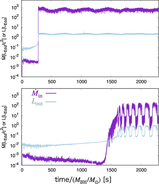
Time evolution of the mass input rates and outgoing radiation luminosities for Model-380 (upper panel) and Model-110 (bottom panel). The purple and blue line represent the mass accretion rate |$\dot{M}_{\,\,\rm in}$| and the luminosity Lout. The luminosities are smaller than the values in table 2, since these are calculated from the first step simulation data, in which the inner edge is set to be at 20rs.
Appendix 2. Angular profiles of density
It may be interesting to compare our results with those of the CDAF or ADAF. We plot the angular density profiles at several radii in figure 13 (by the solid lines), together with those of the CDAF and ADAF (Quataert & Gruzinov 2000). The black dashed line represents the CDAF solution (with n = 0.5, γ = 3/2, where we assume the radial distribution of density to be ρ ∝ r−n) and the dash-dotted line represents the ADAF solution (n = 3/2, γ = 3/2). The normalization of the CDAF and ADAF are chosen arbitrarily.
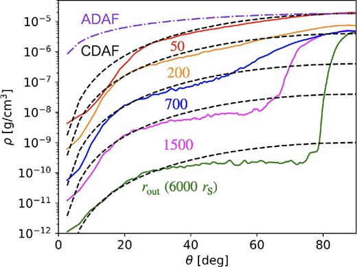
Angular (θ) profiles of the density. The solid lines represent the simulated profiles at various radii: 50rS (red), 200rS (orange), 700rS (blue), 1500rS (pink), and 6000rS (green), respectively. The dashed and dash-dotted lines represent those of CDAF and ADAF, respectively.
It is obvious that the simulated profiles roughly coincide with the CDAF solutions but only at middle angular ranges (20°–50°). The simulated density values are higher (or lower) than those of the CDAF at large (small) θ values. The former indicates the presence of high-density inflow, whereas the latter is due to the outflow effect, which is not taken into account in the analytical solution.
