


Abstract
This paper reports detections of Hα emission and stellar continuum out to approximately 30 physical kiloparsecs, and Hα directionality in the outskirts of Hα-emitting galaxies (Hα emitters) at |$z$| = 0.4. This research adopts narrow-band selected Hα emitters at |$z$| = 0.4 from the emission-line object catalog by Hayashi et al. (2020, PASJ, 72, 86), which is based on data in the Deep and Ultradeep layers of the Hyper Suprime-Cam Subaru Strategic Program. Deep narrow- and broad-band images of 8625 Hα emitters across 16.8 deg2 enable us to construct deep composite emission-line and continuum images. The stacked images show diffuse Hα emission (down to ∼5 × 10⁻²⁰ erg s−1 cm−2 arcsec−2) and stellar continuum (down to ∼5 × 10⁻²² erg s−1 cm−2 Å−1 arcsec−2), extending beyond 10 kpc at stellar masses >109 |$M_\odot$|, parts of which may originate from stellar halos. Those radial profiles are broadly consistent with each other. In addition, we obtain a dependence of the Hα emission on the position angle because relatively higher Hα equivalent width has been detected along the minor-axis towards galaxy disks. While the Hα directionality could be attributed to biconical outflows, further research with hydrodynamic simulations is highly demanded to pin down the exact cause.
1 Introduction
Galaxy outskirts record mass-assembly histories of merger and accretion events in a hierarchical universe (Searle & Zinn 1978; White& Rees 1978), and also feedback processes taking place therein (Dekel & Silk 1986; Heckman et al. 1990). Past deep wide-field imaging uncovered various diffuse stellar halos of nearby galaxies and hence diverse buildup histories of outer disks (Courteau et al. 2011; Deason et al. 2014; Merritt et al. 2016; Harmsen et al. 2017), which correlate with their physical properties (Elias et al. 2018). Combined analyses with simulations in the cosmological framework of Lambda cold dark matter (CDM) claim that, in general, high fractions of inner and outer stellar halos are formed by in-situ and ex-situ stellar components, respectively (Zhang et al. 2018b; Merritt et al. 2020; Font et al. 2020). Furthermore, the diffuse ionized gas and its physical states in the outskirts of nearby galaxies have been well investigated for understanding feedback mechanisms (e.g., Veilleux et al. 2005 and references therein). Zhang et al. (2016, 2018a) successfully detected |$ {H}\alpha + [{N}\, \rm {\small {ii}}]$| emission at |$z$| = 0.05–0.2 out to 100 kpc by combining millions of fiber spectra from the Sloan Digital Sky Survey, providing a unique insight into cool gas from associated halos. However, it remains significantly challenging to observe the galaxy outskirts beyond the local universe due to cosmological surface brightness dimming, which has hampered direct observations to-date from the earlier phase of the mass assembling.
Nowadays, a giant wide-field imager on the Subaru Telescope with an 8.2 m primary mirror, Hyper Suprime-Cam (Miyazaki et al. 2018; Furusawa et al. 2018; Kawanomoto et al. 2018; Komiyama et al. 2018) has enabled very deep wide-field observations under seeing conditions of <1″ that provide new insights into the outskirts of nearby galaxies (Fukushima et al. 2019; Okamoto et al. 2019). In addition, such high-quality imaging data over >100 deg2 taken by Hyper Suprime-Cam Subaru Strategic Program (HSC-SSP; Aihara et al. 2018) can establish even deeper images by stacking numerous objects. This enables us to investigate the outskirts of massive galaxies beyond the local universe (Huang et al. 2018b; Wang et al. 2019), and their environmental dependence (Huang et al. 2018a).
With such scientific backgrounds, this research aims at investigating the outskirts of Hα line emission from star-forming galaxies at |$z$| = 0.4. The Hα line is used extensively as a tracer of star formation (Kennicutt 1998), which helps us study galaxy outskirts from a unique standpoint. Based on the emission-line object catalog available from the Second Public Data Release of HSC-SSP (HSC-SSP PDR2; Aihara et al. 2019; Hayashi et al. 2020), we perform a stacking analysis of Hα line and continuum images for 8625 Hα-emitting galaxies termed as Hα emitters at |$z$| = 0.4. A wide and deep narrow-band survey by HSC-SSP successfully detects Hα emitters at |$z$| = 0.393–0.404 down to ∼1 × 10⁻¹⁷ erg s−1cm−2 over 16.8 deg2 (section 2). We investigate radial profiles of their composite Hα and continuum images in different stellar mass bins, and study star formation in the outskirts of Hα emitters (section 3). We also discuss other possible contributions to Hα emission on the galaxy outskirts by shape-aligned stacked images, and lastly we summarize the entire flow of this work (section 4).
This research adopts the AB magnitude system (Oke & Gunn 1983) and a Chabrier (2003) stellar initial mass function (IMF). Also, we assume cosmological parameters of ΩM = 0.310, |$\Omega _\Lambda =0.689$|, and H0 = 67.7 km s−1 Mpc−1 in a flat Lambda CDM model, which are consistent with those from the Planck 2018 VI results (Planck Collaboration 2020).
2 Data and methodology
The source catalog and data set underlying this paper are available on the HSC-SSP Public Data Release site.1 This section briefly overviews the narrow-band emitter catalog in HSC-SSP PDR2 (Hayashi et al. 2020) and describes our procedure of image stacking of broad-band and narrow-band data for the targets, Hα emitters at |$z$| = 0.4.
2.1 HSC-SSP PDR2
This work is based on the Hα emitter sample at |$z$| = 0.4 established by Hayashi et al. (2020); they reported narrow-band selected emission-line objects at |$z$| < 2 based on the Deep and Ultradeep layers in HSC-SSP PDR2 (Aihara et al. 2019). The catalog contains 8625 Hα emitters down to a limiting flux of ∼1 × 10⁻¹⁷ erg s−1cm−2 (figure 1) and line equivalent width (EW|$_\mathrm{H\alpha +[N\, {\rm \small {ii}}]}$|) of >25 Å in the rest-frame (Hayashi et al. 2020, table 4). They show flux excesses in the narrow band, NB921 (λcenter = 9205 Å), relative to the |$z$| and y bands by capturing Hα (the [N ii] doublet also falls into the filter, however, we omit it hereafter) emission line at |$z$| = 0.393–0.404 (Hayashi et al. 2020, table 3). The survey area covers 22.09 deg2 (16.79 deg2 excluding bright star mask regions) split into four fields (Extended COSMOS, SXDS, ELAIS-N1, and DEEP2-3; Hayashi et al. 2020, table 1). Stellar masses of our sample are derived by Mizuki, a SED-based photo-|$z$| code (Tanaka 2015; Tanaka et al. 2018), by fixing the source redshift of |$z$| = 0.4 (stellar_mass_mizuki_zfixed_convflux in the source catalog; Hayashi et al. 2020).
![Narrow-band (${H}\alpha + [{N\, \rm {\small {ii}}}]$) flux versus logarithmic stellar mass, with stellar mass distributions in the top panel. The light-gray, gray, and black symbols indicate unused emitters in this work, those for the main analysis (section 3), and emitters with high ellipticities (ε > 0.33) that are used in the discussion section (see section 4), respectively. The horizontal line depicts the selection threshold for the narrow-band flux (4 × 10⁻¹⁷ erg s−1cm−2). The dotted vertical lines represent selection cuts into three stellar-mass bins.](https://oup.silverchair-cdn.com/oup/backfile/Content_public/Journal/pasj/74/2/10.1093_pasj_psab127/2/m_psab127fig1.jpeg?Expires=1749356216&Signature=KVQJfZJ5J1q~TXbBHTPk0HbJFRC9az4xdBMlHp~B49hdIm29yvsvO6kfhS137MUwiYDLDQXrysueMLc0yaG~oLLcx4kR89Wxb7tx5ib9oLE1qpD47pYJNVauBULicQptSaOc0C5LH9GOuqSdQsljospdeWsuTUTbptf6mB3~Y-KHwgiS~6aGXxECq0t9YgoKe-O7rUSNR4XNKnehW7LfcgGSEPh4MaTCQuFxRwW8f4PmxJvXfTDKFmvFz~7a-B4ywhR5zdlgte06ME0UjTZQEB6YZf6KxT7NSI1meu3U7wpnffU0XXi634dcCT37NhaSMeNMP3eq3isu-2BFu2nfHQ__&Key-Pair-Id=APKAIE5G5CRDK6RD3PGA)
Narrow-band (|${H}\alpha + [{N\, \rm {\small {ii}}}]$|) flux versus logarithmic stellar mass, with stellar mass distributions in the top panel. The light-gray, gray, and black symbols indicate unused emitters in this work, those for the main analysis (section 3), and emitters with high ellipticities (ε > 0.33) that are used in the discussion section (see section 4), respectively. The horizontal line depicts the selection threshold for the narrow-band flux (4 × 10⁻¹⁷ erg s−1cm−2). The dotted vertical lines represent selection cuts into three stellar-mass bins.
To collect Hα emitters homogeneously across the entire survey area, we set several selection criteria, as follows. We adopt only Hα emitters with narrow-band fluxes greater than 4 × 10⁻¹⁷ erg s−1 cm−2 (SFR = 0.1 |$M_\odot$| yr−1 without dust correction), where the imaging depths achieve approximately |$100\%$| completeness over the whole of the survey fields (Hayashi et al. 2020). Also, this study does not consider areas taken under relatively bad seeing conditions (FWHM |$> {0{^{\prime\prime}_{.}}8}$|) in either the narrow band (NB921) or the |$z$| band. We then select 6324 Hα emitters through these thresholds.
2.2 Stacking analysis
| Sample | Limits | N |
|---|---|---|
| All | fNB > 4 × 10⁻¹⁷, FWHM < 0.8 | 6324 |
| Low-mass | M⋆ = 108–109 | 2121 |
| Mid-mass | M⋆ = 109–1010 | 3139 |
| High-mass | M⋆ = 1010–1011 | 948 |
| Shape-aligned | M⋆ = 109–1011, ε > 0.33 | 1430 |
| Sample | Limits | N |
|---|---|---|
| All | fNB > 4 × 10⁻¹⁷, FWHM < 0.8 | 6324 |
| Low-mass | M⋆ = 108–109 | 2121 |
| Mid-mass | M⋆ = 109–1010 | 3139 |
| High-mass | M⋆ = 1010–1011 | 948 |
| Shape-aligned | M⋆ = 109–1011, ε > 0.33 | 1430 |
See also figure 1 for the selection thresholds.
| Sample | Limits | N |
|---|---|---|
| All | fNB > 4 × 10⁻¹⁷, FWHM < 0.8 | 6324 |
| Low-mass | M⋆ = 108–109 | 2121 |
| Mid-mass | M⋆ = 109–1010 | 3139 |
| High-mass | M⋆ = 1010–1011 | 948 |
| Shape-aligned | M⋆ = 109–1011, ε > 0.33 | 1430 |
| Sample | Limits | N |
|---|---|---|
| All | fNB > 4 × 10⁻¹⁷, FWHM < 0.8 | 6324 |
| Low-mass | M⋆ = 108–109 | 2121 |
| Mid-mass | M⋆ = 109–1010 | 3139 |
| High-mass | M⋆ = 1010–1011 | 948 |
| Shape-aligned | M⋆ = 109–1011, ε > 0.33 | 1430 |
See also figure 1 for the selection thresholds.
In addition, we generate random 100 realizations of composite emission-line and stellar continuum images to measure flux uncertainties of the stacked images using a bootstrap re-sampling from the same samples but with replacements. Based on the 100 random combined images, we calculate a standard deviation of self-flux counts at a given radius. We also derive a background deviation given a pixel area (S) based on randomly positioned empty apertures. The background deviations obtained correlate with the background areas by ∝S∼0.8, suggesting partial pixel-to-pixel correlations (cf. no correlation and full correlation if ∝S0.5 and ∝S, respectively). This research defines the mean square errors of deviations of the self-flux and background noises as a total uncertainty of derived flux surface density (section 3). In addition, residual background counts are sampled by measuring median pixel values in the backgrounds of the randomly combined images. Obtained residual background counts are ∼4 × 10⁻⁴ and ∼4 × 10⁻³ in Hα and continuum images, respectively, in the zero-point magnitude of 27 mag. These residual backgrounds are subtracted when deriving the flux densities.
3 Results
Median radial profiles of Hα emission (ΣFHα) and stellar continuum in three different stellar masses are shown in figure 2, where radial continuum distributions are normalized at the peak surface densities in Hα line. Examples of the composite Hα and continuum images are presented in the Appendix. As a result, we detect both Hα and continuum of the sample in outer regions of Hα emitters at |$z$| = 0.4, especially at the highest stellar mass bin (1010–11 |$M_\odot$|). While we observe differentials between Hα and stellar distributions in ∼10 physical kiloparsecs (ph-kpc) at the highest stellar mass, as is explored in more detail in section 4, they are generally consistent with each other.
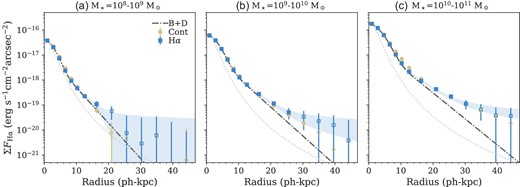
Radial profiles of surface brightness of Hα line emission (blue squares) and normalized stellar continuum (yellow circles) for Hα emitters at |$z$| = 0.4. Less than 2σ detections are represented by the open symbols. The error-bars depict 1σ errors and the light-blue regions are 1σ errors of the curve fitting (see text). From left to right, panels depict radial profiles for Hα emitters with stellar masses of (a) 108–9, (b) 109–10, and (c) 1010–11 |$M_\odot$|, respectively. The dotted curves indicate scaled radial profiles of the composite PSF (fitted by a Moffat distribution). The dot–dashed curves are the best-fitting Gaussian + exponential radial profiles, which are expected to trace bulge + disk components of the Hα emitters. (Color online)
The best-fitting parameters and associated errors for the Hα flux surface densities are summarized in table 2. Figure 2 shows that there are residual components beyond ≳15 ph-kpc compared to the best-fitting bulge + disk profiles in the intermediate and high stellar mass bins (figures 2b and 2c). Such residuals have been commonly observed in stellar distributions of nearby galaxies (e.g., Courteau et al. 2011; Merritt et al. 2016), suggesting that they could originate respectively from in-situ hot young stars and old stars in outer disks and stellar halos (see section 4 for more discussion). The estimated power-law slopes in the outskirts, γ = −1.4 to −1.2, are flatter than those of most nearby galaxies γ < −2 (Harmsen et al. 2017). However, given the low signal detection, it may be too early to conclude that Hα emitters at |$z$| = 0.4 have much shallower power-law slopes than galaxies in the local universe. Recent studies have reported that stellar halo distributions can be fitted by a broken power law; the outer slopes become significantly steeper at broken radii of a few tens of ph-kpc (Deason et al. 2014). This may be one of the reasons of non-detection in both Hα and continuum images at r > 30 ph-kpc.
Best-fitting parameters and 1σ errors in three different stellar mass bins (see figure 2).
| Mass range | 108–109 | 109–1010 | 1010–1011 |
|---|---|---|---|
| (N =) | (2121) | (3139) | (948) |
| Ag (× 10−17) | 3.0 ± 0.2 | 4.9 ± 0.2 | 14.2 ± 0.6 |
| |$w$|g | 11.6 ± 0.5 | 15.9 ± 0.5 | 20.9 ± 0.8 |
| Ae (× 10−17) | 1.3 ± 0.4 | 1.7 ± 0.4 | 3.7 ± 1.0 |
| rs | 3.1 ± 0.3 | 3.8 ± 0.3 | 4.2 ± 0.4 |
| Ap (× 10−18) | 0.6 ± 2.1 | 1.5 ± 2.6 | 11.8 ± 9.1 |
| γ | −1.2 ± 1.3 | −1.2 ± 0.5 | −1.4 ± 0.2 |
Moreover, we convert the Hα surface densities to SFR surface densities (ΣSFR) and investigate fractions of star formation in stellar halos at >10 ph-kpc (figure 3). We follow the Kennicutt (1998) calibration and scale by 1/1.7 to apply the Chabrier (2003) IMF. Also, we assume |$20\%$| contributions of [N ii]λλ6548, 6583 lines to narrow-band fluxes. Here it should be noted that we assume no extinction and do not consider a warm ionized medium (Reynolds et al. 1973; Haffner et al. 2009). Thus, the derived ΣSFR values should have significant uncertainties beyond the measurement errors. In particular, Hα extinction in the central components of emitters would exceed 1 mag at the high stellar mass bin (Sobral et al. 2016). However, central star formation is not the scope of this paper; therefore, we solely focus on the outskirts of Hα emitters. The stacked data have reached ΣSFR down to ∼3 × 10⁻⁶ |$M_\odot$| yr−1 kpc−2, about a half of which appears to originate from stellar halos. As inferred from the best-fitting results, major fluxes beyond 30 ph-kpc are dominated by halo components; however, significant uncertainties are associated with these results.
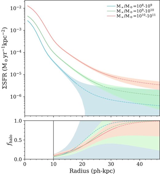
(Top panel) Radial profiles of surface SFR densities of Hα emitters in three stellar mass bins as in figure 1 and table 1 (blue: 108–9, green 109–10, and red: 1010–11 |$M_\odot$|, respectively). (Bottom panel) Fractions of power-law components to the best-fitting radial profiles (fhalo) in respective stellar mass bins at r > 10 ph-kpc. Non-detection regions with <2σ are extrapolated by the best-fitting curves (dashed curves). (Color online)
4 Discussion and summary
This work has identified diffuse Hα emission and stellar continuum beyond 10 ph-kpc and up to 30 ph-kpc for the Hα emitters at |$z$| = 0.4 based on the deep narrow-band and broad-band stacking taken from HSC-SSP. There are residual excesses in both Hα line and stellar continuum compared to exponential distributions at ≳20 ph-kpc. While such residual emissions could originate respectively from in-situ hot young stars and old stars in outer disks and stellar halos, we cannot ignore contributions from associated halos (Zhang et al. 2016, 2018a) and the escape of ionizing radiation (e.g., Leitherer et al. 1995; Heckman et al. 2011). Thus the physical origins of diffuse emission lines are still controversial. In addition, we do not obtain a clear discrepancy between the radial profiles of the emission line and the continuum on the outskirts. The observed Hα surface densities monotonically decline in the outskirts with flatter power-law slopes of γ = −1.4 to −1.2 than those in nearby galaxies; however, we note weak detection of some diffuse stellar halos.
Lastly, we delve into causal factors that may contribute to the observed diffuse Hα emission on the outskirts by constructing shape-aligned composite images of Hα emitters. This is originally motivated to observe diffuse ionized gas arising from biconical outflows from galaxy disks, as typified by the nearby starburst M 82 (e.g., Lynds & Sandage 1963; Visvanathan & Sandage 1972; Bland & Tully 1988; Veilleux et al. 2003; Yoshida et al. 2019). Based on the second moments of the object intensity, termed adaptive moments, we calculate ellipticities (ε) and position angles of the targets (Bernstein & Jarvis 2002). We use the adaptive moments in the i band (i_sdssshape_shape) because the i-band data have better and more homogeneous seeing sizes (|$\sim\!{0{^{\prime\prime}_{.}}6}$|) over the survey field. Also, we employ only elliptic sources at M⋆ > 109 |$M_\odot$| with ε > 0.33 (i.e., major-axis >1.5 × minor-axis) to confirm the credibility of position angle estimates. We align objects along the major-axis; consequently, we conduct the median stacking following a similar method described in subsection 2.2 for 1430 objects that satisfy these selection criteria (see figure 1 and table 1).
Figure 4 represents radial profiles of the rest-frame EWHα along ±30° of the major and minor axes. For deriving radial EWHα profiles appropriately, the color-term correction is important because the color term is significantly different between the major and minor axes. We thus correct the color-term effect in each radial bin on the best effort basis, by using the control sample (see the Appendix for the detailed procedure). The result shows a clear directivity of EWHα; for instance, EWHα is higher on the outskirts along the minor-axis of the stellar disk (figure 4). A possible factor producing such high EWHα could be biconical galactic outflows. However, as discussed above, there are various potential contributions such as star formation in outer disks and emission from associated halos; therefore, the actual cause would be more complex and complicated. On the other hand, the moderate dip in the center can be explained by higher nebular dust extinction and/or a lower specific star formation rate in the galactic bulge.
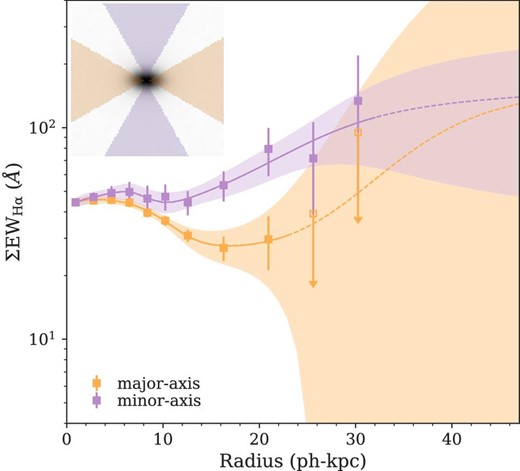
Radial profiles of rest-frame EW of Hα emission in the directions of ±30° from the major-axis (orange symbols) and the minor-axis (purple symbols), respectively. An image illustration of the areas used in the stacking analysis is denoted at the upper left-hand corner. The error-bars and color-filled regions represent 1σ errors. The open symbols indicate 2σ upper limits. The dashed curves depict extrapolated lines of the best-fitting models. (Color online)
In summary, we have unveiled stellar and Hα radial profiles on the outskirts of Hα emitters at |$z$| = 0.4 for the first time. However, contributors to diffuse Hα emission remain uncertain. Comparing our results with hydrodynamic simulations (e.g., Ho et al. 2020; Nelson et al. 2021) and absorption-line observations (e.g., Werk et al. 2014; Prochaska et al. 2017) will help us resolve its causal factors from theoretical and independent points of view, respectively. In addition, more detailed investigations of physical properties of diffuse halos, e.g., derivation of stellar populations on the outskirts based on multi-band image stacking, will deliver further insights into mass-assembly histories surrounding galaxies beyond the local universe.
Acknowledgements
Based on data collected at the Subaru Telescope and retrieved from the HSC data archive system, which is operated by Subaru Telescope and Astronomy Data Center at National Astronomical Observatory of Japan. We are honored and grateful for the opportunity of observing the universe from Mauna Kea, which has the cultural, historical and natural significance in Hawaii.
The Hyper Suprime-Cam (HSC) collaboration includes the astronomical communities of Japan and Taiwan, and Princeton University. The HSC instrumentation and software were developed by the National Astronomical Observatory of Japan (NAOJ), the Kavli Institute for the Physics and Mathematics of the Universe (Kavli IPMU), the University of Tokyo, the High Energy Accelerator Research Organization (KEK), the Academia Sinica Institute for Astronomy and Astrophysics in Taiwan (ASIAA), and Princeton University. Funding was contributed by the FIRST program from Japanese Cabinet Office, the Ministry of Education, Culture, Sports, Science and Technology (MEXT), the Japan Society for the Promotion of Science (JSPS), Japan Science and Technology Agency (JST), the Toray Science Foundation, NAOJ, Kavli IPMU, KEK, ASIAA, and Princeton University. This paper makes use of software developed for the Large Synoptic Survey Telescope. We thank the LSST Project for making their code available as free software at 〈http://dm.lsst.org〉.
The Pan-STARRS1 Surveys (PS1) have been made possible through contributions of the Institute for Astronomy, the University of Hawaii, the Pan-STARRS Project Office, the Max-Planck Society and its participating institutes, the Max Planck Institute for Astronomy, Heidelberg and the Max Planck Institute for Extraterrestrial Physics, Garching, The Johns Hopkins University, Durham University, the University of Edinburgh, Queen's University Belfast, the Harvard-Smithsonian Center for Astrophysics, the Las Cumbres Observatory Global Telescope Network Incorporated, the National Central University of Taiwan, the Space Telescope Science Institute, the National Aeronautics and Space Administration under Grant No. NNX08AR22G issued through the Planetary Science Division of the NASA Science Mission Directorate, the National Science Foundation under Grant No. AST-1238877, the University of Maryland, and Eotvos Lorand University (ELTE) and the Los Alamos National Laboratory.
This research was financially supported by JSPS KAKENHI Grant Number JP19K14766. We would like to thank Editage 〈www.editage.com〉 for English language editing. This work made extensive use of the following tools, NumPy (Harris et al. 2020), Matplotlib (Hunter 2007), lmfit,3 the Tool for OPerations on Catalogues And Tables, TOPCAT (Taylor 2005), a community-developed core Python package for Astronomy, Astopy (Astropy Collaboration 2013), and Python Data Analysis Library pandas (McKinney et al. 2010).
Appendix. Radial color-term dependence
This section describes how we determine the color-term values between the NB921 and |$z$| bands to investigate the Hα directionality for our Hα emitters at |$z$| = 0.4 in section 4. The shape-aligned composite Hα and continuum images of Hα emitters are shown in figure 5, where we assume a fixed color-term value of ζ ≡ fNB/f|$z$| = 1.0375. The original emitter source catalog (Hayashi et al. 2020) applied the color-term correction by using weighted combined zy fluxes, in particular, to separate [O ii] emitters at |$z$| = 1.47 from distant red galaxies at |$z$| ∼ 1.3. However, we decided not to use y-band data in the stacking analyses taking into account its ∼1-mag-shallower imaging depth compared to that in the |$z$|-band. In addition, we detect significantly brighter PSF wings in the y band than in the NB921 and |$z$| bands, which make the issue even more complicated.
![Composite Hα (+ [N ii]) (left) and continuum images of shape-aligned Hα emitters (right) (see section 4). The white circles depict the radius of 30 ph-kpc. Here they are stretched to a logarithmic scale to improve visibility.](https://oup.silverchair-cdn.com/oup/backfile/Content_public/Journal/pasj/74/2/10.1093_pasj_psab127/2/m_psab127fig5.jpeg?Expires=1749356216&Signature=MUkI3L~ErX5zRObdqutJtoP-CQgz~TO1JgOT7aLQKXtU0X0A-mmqJu7xger-OERj3XCR4~YcEN3eWioT6KzN3Em7eYXBDbnjc0UhaGeD1EtLPA4b7-u9SaMiCEDorxnL2EVod5U2vsNE2fGg-ep6LKq-71XGRWoi2ETB00LITny5AT~nFpIgaRQryBQe5Nbx0afI3zBSoXeiKrYBSQT8hb8siXOnVsu0shxHBHg4sumoi1xkJ~gdHdrFBfkuvCzwSkrdlHEkF2R~~n~1JVOR-DTf~5kol5V0v3TaJVzD3CKKDUobRydiYmoydPgzQDs~Fp~UoDpfno9v5rP2BzHS8Q__&Key-Pair-Id=APKAIE5G5CRDK6RD3PGA)
Composite Hα (+ [N ii]) (left) and continuum images of shape-aligned Hα emitters (right) (see section 4). The white circles depict the radius of 30 ph-kpc. Here they are stretched to a logarithmic scale to improve visibility.
Instead, we derive typical color-term values by using 37163 non-emitter samples with similar stellar populations (M⋆ = 109–11 |$M_\odot$| and SFR >0.1 |$M_\odot$| yr−1) at |$z$|photo = 0.3–0.5 in the same field. Their stellar masses, SFRs, and photometric redshifts are obtained from Mizuki SED fitting with reduced chi-squares <5 (Tanaka 2015; Tanaka et al. 2018). The control samples also satisfy the same selection threshold of the shape measurement as for the shape-aligned Hα emitter sample (ε > 0.33). We then generate 100 realizations of shape-aligned stacked NB921 and |$z$| images of 10000 randomly selected non-emitters from the control samples. We here adjust the sampling rates of non-emitters to match the stellar mass distribution to the Hα emitter sample. Based on random composite images, we measure the median color-term values, ζ(r) ≡ fNB(r)/f|$z$|(r), in each radial bin along the major and minor axes (figure 6).
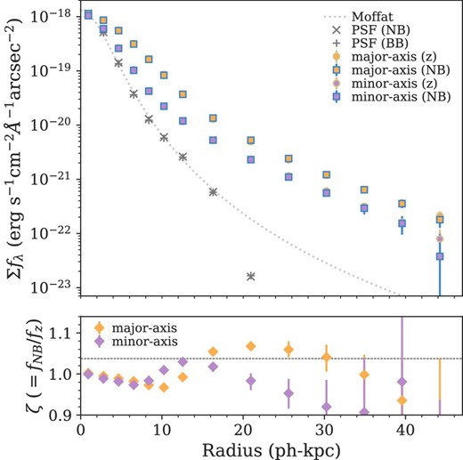
(Top panel) Radial profiles of surface flux densities in NB921 (fNB) and |$z$|-band (fz). The orange squares and circles, respectively, indicate fNB and fz in the major-axis. Similarly, the purple squares and circles show fNB and fz in the minor-axis. The black cross and plus symbols depict composite PSFs in NB921 and |$z$|-band, respectively. The dotted line is the best-fitting Moffat model to the composite PSF in NB921, adopted throughout the paper. (Bottom panel) Radial color term distribution along the major-axis (orange) and minor-axis (purple). In both panels, error-bars indicate |$68\%$| in 100 random realizations. (Color online)
We adopt measured ζ(r) values to obtain color-term-corrected radial profiles of EWHα in the major and minor axes (figure 7). First of all, figure 6 indicates bluer color terms along the major-axis than the minor-axis at ∼10 ph-kpc, which should be caused by disk components of star-forming galaxies. Such a low color term leads to a strange dip of EWHα in the major-axis if we do not consider this effect (figure 7c). The color terms then increase at larger radii where old stellar populations are more dominant. In contrast, they tend to decline at ≳14 ph-kpc in the minor-axis and ≳20 ph-kpc in the major-axis. Such depressions are thought to be simply due to lower signals in NB921. However, one should note that the color-term uncertainties in the faint end do not affect our conclusions given large EWHα errors (figure 7).

(a) Same as in figure 2 but for the major-axis of the shape-aligned composite images. Those with color-term corrections based on ζ(r) derived in figure 6 are shown by blue and yellow open symbols, respectively. (b) Same as in figure 7a, but for the minor-axis. (c) Same as in figure 4, but we here compare radial profiles of EWHα with and without color-term corrections, which are respectively depicted by open symbols with dark-colored regions and filled symbols with light-colored regions. (Color online)
Footnotes
〈https://hsc-release.mtk.nao.ac.jp/das_cutout/pdr3/〉 (registration is required).
M. Newville et al. 2021, lmfit/lmfit-py: 1.0.3 〈https://zenodo.org/record/5570790〉.
References
Author notes
NAOJ Fellow.
