


Abstract
On 2020 December 5 at 17:28 UTC, Japan Aerospace Exploration Agency’s Hayabusa2 sample return capsule (SRC) re-entered Earth’s atmosphere. The capsule passed through the atmosphere at supersonic speeds, emitting sound and light. The inaudible sound was recorded by infrasound sensors installed by Kochi University of Technology and Curtin University. Based on analysis of the recorded infrasound, the trajectory of the SRC in two cases, one with constant-velocity linear motion and the other with silent flight, could be estimated with an accuracy of |${0{_{.}^{\circ}}5}$| in elevation and 1° in direction. A comparison with optical observations suggests a state of flight in which no light is emitted but sound is emitted. In this paper, we describe the method and results of the trajectory estimation.
1 Introduction
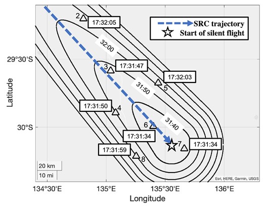
Meteoroids passing through the atmosphere at supersonic speeds generate shock waves (ReVelle 1976). Studies have calculated the trajectories of fireball (bright meteors) from seismometer measurements of the associated shock waves (Nagasawa 1987; Ishihara et al. 2003, 2004). Re-entry capsules passing through the atmosphere also generate shock waves, as observed for Stardust (Desai et al. 1999; ReVelle & Edwards 2007), Genesis (ReVelle et al. 2005) and Hayabusa (Yamamoto et al. 2011; Ishihara et al. 2012) during their atmospheric re-entry. It has been suggested that it may be possible to estimate the trajectory and speed of an object from measurements of the sound it emits (Lonzaga et al. 2015). The asteroid explorer Hayabusa2, launched by the Japan Aerospace Exploration Agency (JAXA) on 2014 December 3, arrived at the asteroid Ryugu in 2018 and collected surface rocks during two touch downs (on 2019 February 22 and July 11) (Tsuda et al. 2019, 2020). The collected samples were stored in a sample return capsule (SRC), which re-entered Earth’s atmosphere at around 17:28 (UTC) on 2020 December 5, and successfully landed in South Australia. Infrasound sensors (INF04LE micro-atmospheric vibrometers, see below) at seven sites (four sensors at each site, for a total of 28 sensors) along the re-entry trajectory (figure 1) installed by Kochi University of Technology, Japan, and Curtin University, Australia, detected the infrasound generated by the SRC as it passed through the atmosphere. Many infrasound sensors were deployed to establish a temporary sensor network. At the time of the Hayabusa1 re-entry in 2010, we deployed only five infrasound sensors (Model 2 and Model 25, Chaparral Physics).
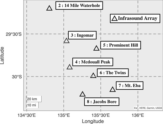
Layout of infrasound sensors installed near nadir of the SRC re-entry trajectory.
Since then, we have been developing original infrasound sensors in collaboration with a manufacturing company (SAYA Inc., Japan). A small chamber electromagnetically coupled to simple membranes is used to measure sounds in the range of 6.25 Hz down to 0.001 Hz (SAYA INF01LE) and multiple capacitance microphones are used to measure sounds in the range of 0.05 Hz up to the audible range (SAYA INF04LE). Since 2016, the INF01LE sensors have been deployed in Japan to monitor meteorologically and/or event-driven variation of infrasound to estimate the energy deposition of geophysical events such as tsunamis, volcanic eruptions, and thunderstorms, and its propagation characteristics in the atmosphere (Batubara & Yamamoto 2020; Hamama & Yamamoto 2021; Saito et al. 2021). The data from the 28 INF04LE sensors, which are portable and have low power consumption, used in this study were recorded by Raspberry Pi data loggers (Sansom et al. 2022). The numbering of the locations of the infrasound sensors used here follows that used by Sansom et al. (2022), where the seven locations are numbered from 2 to 8. At a given location, one sensor was placed at the center and the other three sensors were placed at the vertices of an equilateral triangle, each 100 m from the center. The time of arrival of a shock wave depends on the location of the installed infrasound sensor. It is recorded by the sensor as an N-type signal (Langston 2004), as shown in figure 2.
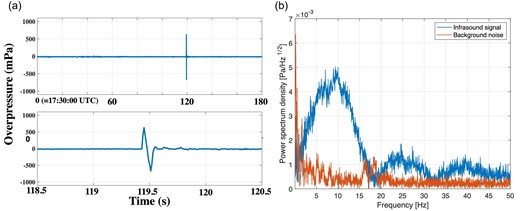
Examples of observed infrasound, recorded in the 0.01–50 Hz band. (a) Overpressure versus time, at Jacobs Bore (|${30{^{\circ}_{.}}21261 }$|S, |${135{^{\circ}_{.}}25473 }$|E), where the infrasound shock waves reached at around 119 s from 17:28:00 UTC, and magnified view of recorded N-type signal (bottom panel). (b) Power spectrum density of infrasound signal and background noise. The signal has a peak at 10 Hz. (Color online)
In this study, the return trajectory and behavior of the SRC in the atmosphere were determined by comparing the observed infrasound data with the calculated arrival time of the shock wave. Based on a comparison of the calculated wavefronts with the locations of the infrasound sensors, we suggest the possibility of silent flight (here we refer to the flight of a fireball that is acoustically silent as silent flight, because there is a state in which the fireball is emitting sound; see subsection 4.3) and propose more accurate descriptions of the SRC behavior in the atmosphere and the propagation of shock wavefronts by taking into account the effect of silent flight. In general, the flight of a fireball without the emission of light is called dark flight. Past studies have not clearly differentiated between the inaudible (silent) and invisible (dark) flights.
2 Method
Usually, the shape of a shock wave can be simply determined from the speed of sound and that of the supersonic object, which are obtained from the arrival times of sound waves recorded by multiple infrasound sensors distributed on the ground. The speed of sound is uniform [305 (m s−1) in this study] because of the shallow entry angle of the SRC. Under the assumption that the speeds of sound and the object are constant during the descent, the shape of the wavefront can be treated as a cone (Mach cone). Hayabusa2 passing through the upper atmosphere at a shallow angle is consistent with this assumption, which is thus adopted in this paper.

Diagram of the (X, Y, Z) coordinate system, obtained by rotating and translating the (x, y, z) coordinate system. The Z-axis coincides with the trajectory of Hayabusa2 SRC. γ and θ are the cardinal direction and elevation angle, respectively. The trajectory is broken into three chunks: “bright flight”, “dark flight”, and “silent flight”. Silent flight was observed to last one second longer than dark flight (see subsection 4.3). (Color online)
3 Results
We varied each parameter over a wide range and used the χ2 test to find the optimal parameter set (table 1).
Search domain, grid interval, and optimal value for each parameter.*
| Parameter | Search domain | Grid interval | Optimal value | Error |
|---|---|---|---|---|
| v0 (km s−1) | 10 to 40 | 1.0 | 21 | −4/+6 |
| x0 (km) | −600 to −200 | 1.0 | −483 | −7/+8 |
| y0 (km) | 200 to −600 | 1.0 | 482 | −7/+7 |
| γ (°) | 3 to 15 | 0.5 | 4.0 | −0.5/+0.5 |
| θ (°) | 215 to 225 | 0.5 | 222.5 | −0.5/+0.5 |
| t0 (s) | −50 to 50 | 1.0 | 22 | −5/+5 |
Origin is (30°S, 135°E, 0) at |${17^{\rm h}30^{\rm m}00{^{\rm s}}}$| UTC.
From these optimum values, the arrival wave lines of the shock wave and the trajectory of the SRC can be drawn as shown in figures 4 and 5.
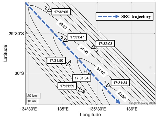
Calculated propagation of shock wavefront projected on to the ground. The times in black frames indicate the arrival times of the shock wave at the corresponding sensors. The arrow indicates the SRC trajectory. The parabola shows the wavefront of the shock wave every 10 seconds. The times without black frames indicate the arrival times of the wavefront. The shape of the wavefront is an oblique cut on the surface of the Mach cone and is thus part of a parabola. Its direction of propagation is opposite to that of the descending SRC. (Color online)
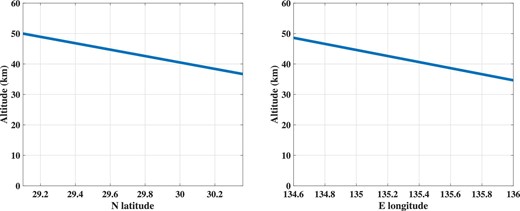
Calculated elevation change of SRC. The SRC moves from northwest to southeast with an elevation angle of 4° and gradually loses altitude. It passes over the infrasound sensors at an altitude of about 35–50 km. (Color online)
Comparing the results of these calculations with the observations, the timing residuals are within three seconds at all observation points (table 2).
Observed and calculated arrival times of shock waves.
| Site number | Site | Observed | Calculated | Timing residual |
|---|---|---|---|---|
| 2 | 14 Mile Waterhole | 17:32:04.9 | 17:32:03.9 | 1.0 |
| 3 | Ingomar | 17:31:46.8 | 17:31:47.3 | −0.5 |
| 4 | Mcdouall Peak | 17:31:50.5 | 17:31:49.5 | 1.0 |
| 5 | Prominent Hill | 17:32:02.9 | 17:32:03.5 | −0.6 |
| 6 | The Twins | 17:31:33.8 | 17:31:36.2 | −2.4 |
| 7 | Mt. Eba | 17:31:34.2 | 17:31:32.1 | 2.1 |
| 8 | Jacobs Bore | 17:31:59.3 | 17:31:59.2 | 0.1 |
4 Discussion
4.1 Silent flight effect
In this paper, trajectory calculations were performed using the grid-search-based method and the best values were obtained using the χ2 test. The value of χ2 was 0.133; however, if we ignore the data obtained at Mt. Eba (site no. 7), the value of χ2 decreases sharply to 0.0012. This indicates that the handling of the data obtained at Mt. Eba was not appropriate. Mt. Eba is the most southeasternly site, and thus the last site that the capsule passed over. Therefore, any change in the behavior of the capsule just before it passed over Mt. Eba could explain the large error in the obtained data.
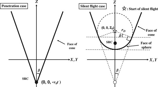
Geometries of shock wave surface. In the penetration case, where the SRC continues its constant velocity linear motion, the shock wavefront is shaped like a cone. In the silent flight case, where the SRC decelerates rapidly at (0, 0, ZD), the shock wavefront is shaped like a combination of a cone and a sphere.
After the onset of silent flight, the shock wave is spherical, and thus the surface of the shock wave looks like a combination of a cone and a sphere. If the silent flight starts between The Twins and Mt. Eba, the shock wave that arrives at Mt. Eba may be delayed (figure 7). We searched for the optimal value in a similar way to the calculation of the penetration case (table 3). In this silent flight case, the value of χ2 is 0.0084, which is smaller than |$7\%$| of that in penetration case. The calculated arrival times are thus likely to be closer to the observed arrival times in the silent flight case (table 4) compared to the penetration case (table 2).
Calculated propagation of shock wavefront in the silent flight case. The times in black frames indicate the arrival times of the shock wave at the corresponding sensors. The arrow indicates the SRC trajectory. The parabola shows the wavefront of the shock wave every 10 seconds. The times without black frames indicate the arrival times of the wavefront. The wavefronts of the shock wave are shaped like a combination of parabolas and circles. The silent flight began in the sky between the sixth (The Twins) and seventh (Mt. Eba) sensor sites. The error in this silent flight case is much smaller than that in the penetration case. (Color online)
Search domain, grid interval, and optimal value of each parameter for silent flight case.*
| Parameter | Search domain | Grid interval | Optimal value | Error |
|---|---|---|---|---|
| v0 (km s−1) | 10 to 40 | 1.0 | 12 | −3/+1 |
| x0 (km) | −600 to −200 | 1.0 | −310 | −8/+8 |
| y0 (km) | 200 to 600 | 1.0 | 314 | −7/+7 |
| γ (°) | 3 to 15 | 0.5 | 5.5 | −0.5/+0.5 |
| θ (°) | 215 to 225 | 0.5 | 221.5 | −1 /+1 |
| t0 (s) | −50 to 50 | 1.0 | 2 | −6/+6 |
| tD (s) | −60 to 20 | 1.0 | −33 | −1/+1 |
Origin is (30°S, 135°E, 0) at |${17^{\rm h}30^{\rm m}00{^{\rm s}}}$| UTC.
Observed and calculated arrival time of shock waves for silent case.
| Site number | Site | Observed | Calculated | Timing residual |
|---|---|---|---|---|
| 2 | 14 Mile Waterhole | 17:32:04.9 | 17:32:04.7 | 0.2 |
| 3 | Ingomar | 17:31:46.8 | 17:31:47.0 | −0.2 |
| 4 | Mcdouall Peak | 17:31:50.5 | 17:31:49.8 | 0.7 |
| 5 | Prominent Hill | 17:32:02.9 | 17:32:03.2 | −0.3 |
| 6 | The Twins | 17:31:33.8 | 17:31:33.3 | 0.5 |
| 7 | Mt. Eba | 17:31:34.2 | 17:31:34.1 | 0.1 |
| 8 | Jacobs Bore | 17:31:59.3 | 17:31:59.2 | 0.1 |
According to this calculation, the dark flight started at an altitude of about 39 km, and the trajectory of the SRC after that start cannot be estimated (figure 8).
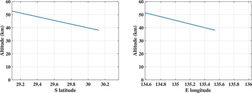
Calculated elevation change of SRC. The SRC moves from northwest to southeast with an elevation angle of 5.5° and gradually loses altitude. It passes over the infrasound sensors at an altitude of about 53 km and transitions to silent flight at an altitude of about 39 km. The movement after the transition to silent flight cannot be inferred from the infrasound data. (Color online)
In this calculation, the trajectory is described more accurately because one infrasound sensor was affected by silent flight. If more than one sensor had been affected by silent flight, an even more accurate calculation could have been made.
4.2 Correction of elevation angle
According to JAXA’s reporter briefing, the atmospheric interference for the SRC is about 200 km in altitude with an approach angle of 12° (JAXA Hayabusa2 Project 2020).1 This approach angle (12°) differs significantly from the elevation angle of 5° calculated in this study. This difference can be explained by the refraction of sound waves by the atmosphere and the roundness of Earth. When sound moves from a slower-velocity layer to a faster-velocity layer, the refraction angle becomes shallower and the elevation angle appears shallower than it should be. This effect is modified by the vertical structure of the atmosphere. The structure of the atmosphere above the SRC during re-entry is shown in figure 9. At an elevation angle of about 5°, the SRC is observed to have an elevation angle of about |${0{_{.}^{\circ}}5}$|–|${1{^{\circ}_{.}}0 }$|, smaller than it would be if the capsule had reached the ground from 40–60 km above.
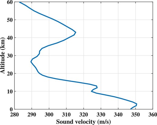
Thermodynamic sound speed profile over sites of Hayabusa2 re-entry on ground. The profile was estimated using |${c}_{th} = \sqrt{\gamma RT}$| (Garcés et al. 1998), where γ (ratio of specific heats) =1.4, R (specific gas constant for dry air) =286.9 J kg−1 K−1 and temperature T were extracted from the MERRA-2 dataset.2 (Color online)
4.3 Comparison with optical observation
We have thus far discussed only the sound data recorded by infrasound sensors. In this subsection, we compare the results with optical observations to verify their validity.
Kochi University of Technology and Curtin University detected infrasound generated by the SRC by installing a temporary scientific observation network under the expected trajectory. In addition to the infrasound sensors, cameras, seismic sensors, and antennas were installed. The trajectory estimated based on optical observations is similar to that estimated based on infrasound data (figure 10). The former was about 10 km ahead of the latter and was not visible (dark flight).
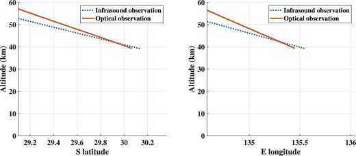
Calculated elevation change of SRC. The blue dotted line and the red line are the trajectories determined from infrasound and optical observations, respectively. (Color online)
We calculated the shock wave arrival time at each observation site based on the optical trajectory. The results are shown in table 5. The arrival times are in good agreement except for that for Mt. Eba. The calculation results are very close to the case where the silent flight started one second earlier.
Observed and calculated (based on optical trajectory) arrival times of the shock wave.
| Site number | Site | Observed | Calculated | Infrasound delayed by 1 s |
|---|---|---|---|---|
| 2 | 14 Mile Waterhole | 17:32:04.9 | 17:32:06.5 | 17:32:04.5 |
| 3 | Ingomar | 17:31:46.8 | 17:31:48.2 | 17:31:47.0 |
| 4 | Mcdouall Peak | 17:31:50.5 | 17:31:49.2 | 17:31:49.9 |
| 5 | Prominent Hill | 17:32:02.9 | 17:32:04.3 | 17:32:03.1 |
| 6 | The Twins | 17:31:33.8 | 17:31:34.1 | 17:31:33.7 |
| 7 | Mt. Eba | 17:31:34.2 | 17:31:53.0 | 17:31:50.7 |
| 8 | Jacobs Bore | 17:31:59.3 | 17:31:56.3 | 17:31:59.4 |
This difference in arrival time can be explained by the difference between dark and silent flights. The results suggest that after the SRC became optically transparent and entered dark flight, it remained acoustically opaque for about one second, travelling about 10 km before entering silent flight.
5 Conclusion
This study used data from 28 sensors installed at locations over which the Hayabusa2 SRC passed to investigate the infrasound generated by the SRC as it travelled at supersonic speed through the atmosphere. Based on an analysis of the arrival time of the observed infrasound, the trajectory of the SRC was calculated. The existence of silent flight was suggested for obtaining more accurate results. The azimuth of the trajectory of the SRC from the north is |${41{^{\circ}_{.}}5 }$| (counterclockwise) and the elevation angle was |${5{^{\circ}_{.}}5 }$|. The capsule passed through the atmosphere and emitted a shock wave until it was about 39 km above the ground, at which point it began silent flight. The results suggest that the behavior of an object moving supersonically in the atmosphere can be determined from infrasound observations at multiple sites with a certain degree of accuracy. The calculated trajectory is consistent with JAXA’s report and with optical observation and suggests that there is a sounding path (without light emission) of about 10 km for about one second before subsonic. Infrasound observations can be performed even in cloudy weather and daytime, and do not require any radio signals from the object. They are thus expected to play a role in the tracking of future atmospheric re-entry objects.
Acknowledgements
Although the Japanese infrasound team could not go to Australia because of COVID-19 restrictions, volunteers made the observation a success. We would like to thank Martin Cupák and the DFN team as well as Geoffrey Bonning, Andrew Cool, Karen Donaldson, Glyn Donaldson, Michael Roche, Terrence Wardle, and Yuta Hasumi for their support, without which this study would not have been finished. We are also indebted to JAXA’s Hayabusa2 Project Team. The authors are grateful for the support from Woomera Test Range, in particular Guy Mold and Colin Telfer; and the Defence Science and Technology Group, in particular Kruger White and team.
Funding
This research was made possible largely through grants from The Murata Science Foundation (grant number M20AN115) and NEXCO Group Companies’ Support Fund to Disaster Prevention Measures on Expressways. MYY would like to acknowledge their support from both fundings. The Desert Fireball Network team is funded by the Australian Research Council under grant DP200102073. EKS would like to acknowledge funding from the Institute of Geoscience Research and the Curtin Faculty of Science and Engineering.
Conflict of interest
The authors declare no conflict of interest.
Footnotes
JAXA Hayabusa2 Project 2020, Reporter briefing: Asteroid explorer, Hayabusa2, 〈https://www.hayabusa2.jaxa.jp/enjoy/material/press/Hayabusa2_Press_20201130_ver8_en2.pdf 〉.
Global Modeling and Assimilation Office (GMAO) 2015, MERRA-2 inst3_3d_asm_Np: 3d,3-Hourly,Instantaneous,Pressure-Level,Assimilation,Assimilated Meteorological Fields, V5.12.4 〈https://disc.gsfc.nasa.gov/datasets/M2I3NPASM_5.12.4/summary 〉.
