


Abstract
We use the Hyper Suprime-Cam Subaru Strategic Program S19A shape catalog to construct weak lensing shear-selected cluster samples. From aperture mass maps covering ∼510 deg2 created using a truncated Gaussian filter, we construct a catalog of 187 shear-selected clusters that correspond to mass map peaks with signal-to-noise ratio larger than 4.7. Most of the shear-selected clusters have counterparts in optically selected clusters, from which we estimate the purity of the catalog to be higher than 95%. The sample can be expanded to 418 shear-selected clusters with the same signal-to-noise ratio cut by optimizing the shape of the filter function and by combining weak lensing mass maps created with several different background galaxy selections. We argue that dilution and obscuration effects of cluster member galaxies can be mitigated by using background source galaxy samples and adopting a filter function with its inner boundary larger than about 2′. The large samples of shear-selected clusters that are selected without relying on any baryonic tracer are useful for detailed studies of cluster astrophysics and cosmology.
1 Introduction
Clusters of galaxies are the most massive gravitationally bound objects in the Universe and have proven to be a key class of objects for establishing the standard cosmological model that consists of dark matter and dark energy (for reviews, see, e.g., Allen et al. 2011; Kravtsov & Borgani 2012). We can study the internal structure and statistical properties of clusters of galaxies with multi-wavelength datasets, including optical, X-ray, and radio. For instance, a massive cluster of galaxies can be securely identified from an overdensity of cluster member galaxies with similar colors (e.g., Gladders & Yee 2000). X-rays from hot gas in clusters of galaxies provide an important means of finding and studying clusters of galaxies (e.g., Ebeling et al. 2001). Large samples of clusters are being constructed via the Sunyaev–Zel’dovich effect on cosmic microwave background fluctuations (e.g., Planck Collaboration 2016; Hilton et al. 2021).
The abundance and internal structure of clusters of galaxies are mainly determined by the dynamics of dark matter, which makes it critically important to study the distribution of dark matter in clusters in great detail. Weak gravitational lensing directly probes the dark matter distribution in clusters of galaxies and hence plays a key role in characterizing clusters (for a review see, e.g., Umetsu 2020). Among others, weak gravitational lensing plays an essential role in the use of the cluster population as a probe of cosmological parameters, because cluster observables must be linked to cluster masses in order to compare the observed abundance of clusters with theoretical predictions (for a review, see, e.g., Pratt et al. 2019). Indeed, attempts to use clusters as an accurate cosmological probe have often been hampered by the uncertainty of mass calibrations of clusters for which complicated selection biases in cluster surveys must be taken into account.
A new approach that has been explored less extensively is finding clusters directly from weak gravitational lensing shear data by identifying peaks in weak lensing mass maps (e.g., Schneider 1996; White et al. 2002; Hamana et al. 2004; Hennawi & Spergel 2005; Maturi et al. 2005, 2010; Fan et al. 2010; Marian et al. 2012; Lin et al. 2016). The abundance of the peaks contains information on the abundance of massive dark matter halos and hence on cosmological parameters (e.g., Jain & Van Waerbeke 2000; Dietrich & Hartlap 2010; Maturi et al. 2010; Shan et al. 2014; Liu et al. 2015a, 2015b; Hamana et al. 2015; Kacprzak et al. 2016; Shan et al. 2018). In addition, the relatively simple and clean selection function of weak lensing shear-selected clusters (e.g., Hamana et al. 2012; Chen et al. 2020) enables their use for better understanding of cluster astrophysics. For instance, X-ray analysis of shear-selected clusters suggests that they tend to be X-ray underluminous compared with clusters found in other techniques (Giles et al. 2015; Miyazaki et al. 2018b).
However, a challenge lies in the requirement of wide and deep imaging for finding a significant number of weak lensing shear-selected clusters. First attempts identified only a handful of such clusters, if restricted to those with a sufficiently high signal-to-noise ratio (see, e.g., the Appendix) of ≳5 (Wittman et al. 2001, 2006; Miyazaki et al. 2002, 2007; Hetterscheidt et al. 2005; Schirmer et al. 2007; Gavazzi & Soucail 2007; Utsumi et al. 2014). On the other hand, more systematic search of weak lensing shear-selected clusters is made possible thanks to recent progress in wide-field imaging surveys. For instance, Shan et al. (2012) constructed a sample of 51 shear-selected clusters with signal-to-noise ratios larger than 4.5 from the Canada-France-Hawaii Telescope Legacy Survey (Heymans et al. 2012).
Hyper Suprime-Cam (HSC; Miyazaki et al. 2018a), which is a wide-field optical imager mounted on the Subaru 8.2 m telescope, offers a unique opportunity for constructing a large sample of weak lensing shear-selected clusters (Miyazaki et al. 2015). In particular, the HSC Subaru Strategic Program (HSC-SSP; Aihara et al. 2018a, 2018b, 2019), which is a deep multi-band imaging survey of 1400 deg2 of the sky, is an ideal survey for this purpose. Miyazaki et al. (2018b) presented a sample of 65 weak lensing shear-selected clusters with signal-to-noise ratios larger than 4.7 from the HSC-SSP first-year shape catalog covering ∼160 deg2 (Mandelbaum et al. 2018b). Using the same HSC S16A data, Hamana, Shirasaki, and Lin (2020) constructed a sample of 124 shear-selected clusters with signal-to-noise ratios larger than 5 by mitigating the dilution effect of foreground and cluster member galaxies.
In this paper, we present updated catalogs of weak lensing shear-selected clusters from the latest HSC-SSP S19A shape catalog covering ∼433 deg2 (X. Li et al. in preparation). We construct catalogs using three different approaches adopting different shapes of filters. We also assign redshifts of individual clusters by cross-matching the shear-selected clusters with optically selected clusters.
This paper is organized as follows. The data used for our analysis are summarized in section 2. Our method for constructing mass maps is detailed in section 3. We present our main results in section 4, and conclude in section 5. Throughout the paper we assume the matter density Ωm = 0.3, the cosmological constant |$\Omega _\Lambda =0.7$|, the baryon density Ωb = 0.05, the dimensionless Hubble constant h = 0.7, the spectral index ns = 0.96, and the normalization of the matter power spectrum σ8 = 0.81.
2 Data
2.1 Weak lensing shape catalog
The HSC-SSP S19A shape catalog (X. Li et al. in preparation) is constructed in a manner similar to the HSC-SSP S16A shape catalog presented in Mandelbaum et al. (2018b) that takes the moment-based approach of Hirata and Seljak (2003). The multiplicative and additive biases are derived with realistic image simulations (Mandelbaum et al. 2018a). The detailed systematics tests presented in X. Li et al. (in preparation) indicate that the S19A shape catalog is sufficiently accurate and is ready for various cosmological and astrophysical analyses. The catalog contains ∼36 million galaxies.
Throughout the paper we adopt the dNNz photometric redshift measurement (A. J. Nishizawa et al. in preparation) for defining background galaxy samples with the P-cut method. This is based on the multiple-layer perceptron that consists of six hidden layers where each layer contains 100 nodes. Input attributes are cmodel magnitude, size, and point spread function matched aperture magnitude in five broad bands, leading to 15 attributes in total, for each galaxy. The outputs are probabilities of the galaxy lying at the redshift bin spanning from z = 0 to 7 divided into 100 bins. The code is trained to minimize the total difference between the output probabilities and input delta-function-like probability summed over all training sample and redshift ranges. From the analysis on the test sample that has not been used for training, it is found that redshifts are accurate with a bias of 10−4, scatter of |$3\%$|, and outlier fraction of less than |$10\%$|. dNNz can avoid overfitting even when part of the data is missing (e.g., due to the lack of images in some broadband filters), by introducing a dropout layer right after an input layer with missing rate 0.2. When applying dNNz on real data, dNNz with the dropout layer is applied only when part of the data is missing, otherwise dNNz without the dropout layer is employed for the complete data to maximize the performance of the photometric redshift measurement.
2.2 Optically selected cluster catalogs
We use several optically selected cluster catalogs to assign redshifts for individual peaks in weak lensing mass maps. First, we adopt a cluster catalog (S20A version 11) constructed with the photometric data from the HSC-SSP S20A internal data release using the CAMIRA algorithm (Oguri 2014). In Oguri et al. (2018a), the CAMIRA algorithm was applied to the HSC-SSP S16A data covering ∼230 deg2 to construct a catalog of 1921 clusters at redshift 0.1 < z < 1.1 and richness N greater than 15 (for the definition of richness N in the CAMIRA algorithm, see Oguri 2014). In this paper, we adopt an updated catalog of 8910 clusters at redshift 0.1 < z < 1.38 and richness greater than 15 from the HSC-SSP S20A data covering ∼830 deg2.
Since the HSC-SSP survey region is chosen to overlap with the Sloan Digital Sky Survey (SDSS; York et al. 2000), we also use SDSS cluster catalogs for assigning cluster redshifts. Specifically, we use the redMaPPer cluster catalog (Rykoff et al. 2014) that contains clusters at 0.08 < z < 0.6 as well as the WHL15 cluster catalog (Wen et al. 2012; Wen & Han 2015) that contains clusters at 0.05 < z < 0.79. Both of these cluster catalogs were constructed based on the photometric galaxy catalog covering ∼14000 deg2 from SDSS Data Release 8 (DR8; Aihara et al. 2011). In addition to these purely optically selected clusters, we also adopt the CODEX cluster catalog (Finoguenov et al. 2020) that contains clusters at 0.05 < z < 0.69 from the ROSAT all-sky survey (RASS; Voges et al. 1999) with optical confirmations using the redMaPPer algorithm applied to the SDSS DR8 data. Throughout the paper we use X-ray centroids as centers of the CODEX clusters.
All the cluster redshifts we adopt throughout this paper are photometric redshifts of clusters derived from the HSC grizy-band photometry for CAMIRA or from the SDSS ugriz-band photometry for redMaPPer, WHL15, and CODEX. The typical accuracy of these cluster photometric redshifts is σz/(1 + z) ∼ 0.01, which is sufficiently accurate for our current purpose.
3 Mass maps
3.1 Introduction
In this paper, we consider two types of spatial filter. One is a truncated Gaussian filter, which resembles the one adopted by Miyazaki et al. (2018b) to construct a shear-selected cluster sample from the HSC S16A data (see also Hamana et al. 2020). The other is a filter introduced by Schneider (1996), which we call a truncated isothermal filter throughout the paper and is designed to optimize the detection of halos from mass maps. In the following subsections we describe these filters in more detail.
3.2 Truncated Gaussian filter
3.3 Truncated isothermal filter
This filter has several desirable properties. First, we can tweak the shape of the filter quite flexibly by adjusting the three parameters ν1, ν2, and θR. Second, it has Q(θ) = 0 at θ < ν1θR and hence allows us to efficiently remove the contribution from the innermost part of halos, which is a source of various systematic effects on the signal such as the dilution effect by cluster member galaxies, the effect of reduced shear, and the magnification bias. Third, the filter is confined within a finite radius [i.e., U(θ) = Q(θ) = 0 at θ > θR] and hence mitigates the impact of, e.g., the boundary of the survey region on the map.
To explore the impact of the different inner boundary of the filter, ν1θR, in this paper we consider two different values of the inner boundary, |$\nu _1\theta _R= {0{^{\prime }_{.}}5}$| and 2′, which are referred as TI05 and TI20, respectively. For both TI05 and TI20, we construct mass maps with four different source galaxy subsamples defined using photometric redshifts of source galaxies (see subsection 2.1), in order to enhance the detection efficiency particularly at high redshifts (see also Hamana et al. 2020). For each inner boundary of the filter and source galaxy sample, we carefully choose parameter values of the filter to maximize the expected signal-to-noise ratio and to mitigate the impact of density fluctuations along the line of sight on cluster finding. The specific procedure for optimization of the parameters is detailed in the Appendix. Table 1 summarizes the set-ups for constructing shear-selected cluster samples. The shapes of the kernel function Q(θ) used in this paper are also presented in figure 1.
![The kernel function Q(θ), which is used to derive the aperture mass map [see equation (4)]. The solid, dashed, and dash-dotted lines are Q(θ) for the TG15, TI05, and TI20 set-ups summarized in table 1. Note that we adopt slightly different shapes of Q(θ) for different source galaxy selections. We show Q(θ) normalized by its maximum value. (Color online)](https://oup.silverchair-cdn.com/oup/backfile/Content_public/Journal/pasj/73/4/10.1093_pasj_psab047/2/m_psab047fig1.jpeg?Expires=1749580301&Signature=qgOESorkupur3UIkMfPKjXEt4ZP0UEsgmxGZ9lDdh3rbGAddxW1O2ILf8czIsh5wvPZBRxyyYy~Dxdply4ANsreASzOcIZY0hz9oKMKVkklhVfpmrNeHKgXM9nZ68KV8awG~j2njBMgUKxhYZPAk7QUIaUg6WtSMkJ26d0q8BHv8JGYDoZFGJXJ49pomSPde55lpu-o6zr7Jg09ZOrp064WZ9ppWZ0mWFSjU6pCfFc-uWFanDnIFJkoa53r8QkXN7wppLUbY63pymX55ZKM-s3gdl~jp-A7OIkHE~IFUW95lfQ56cvlz7sziml7bLNy02tXs45VmFp5m1Ln~WHbcrw__&Key-Pair-Id=APKAIE5G5CRDK6RD3PGA)
The kernel function Q(θ), which is used to derive the aperture mass map [see equation (4)]. The solid, dashed, and dash-dotted lines are Q(θ) for the TG15, TI05, and TI20 set-ups summarized in table 1. Note that we adopt slightly different shapes of Q(θ) for different source galaxy selections. We show Q(θ) normalized by its maximum value. (Color online)
Summary of set-ups to construct shear-selected cluster samples.
| Name | Filter | Parameter values | Source galaxy selection | Num. galaxies |
|---|---|---|---|---|
| TG15 | Truncated Gaussian | |$\theta _0= {1{^{\prime }_{.}}5}$|, θout = 13′ | No cut | 35804886 |
| TI05 | Truncated isothermal | ν1 = 0.021, ν2 = 0.36, |$\theta _R= {23{^{\prime }_{.}}8}$| | zmin = 0.2, zmax = 7, Pth = 0.95 | 32750421 |
| Truncated isothermal | ν1 = 0.025, ν2 = 0.36, |$\theta _R= {20{^{\prime }_{.}}0}$| | zmin = 0.3, zmax = 7, Pth = 0.95 | 26024748 | |
| Truncated isothermal | ν1 = 0.027, ν2 = 0.36, |$\theta _R= {18{^{\prime }_{.}}5}$| | zmin = 0.5, zmax = 7, Pth = 0.95 | 20664165 | |
| Truncated isothermal | ν1 = 0.027, ν2 = 0.36, |$\theta _R= {18{^{\prime }_{.}}5}$| | zmin = 0.7, zmax = 7, Pth = 0.95 | 15564223 | |
| TI20 | Truncated isothermal | ν1 = 0.095, ν2 = 0.36, |$\theta _R= {21{^{\prime }_{.}}1}$| | zmin = 0.2, zmax = 7, Pth = 0.95 | 32750421 |
| Truncated isothermal | ν1 = 0.110, ν2 = 0.36, |$\theta _R= {18{^{\prime }_{.}}2}$| | zmin = 0.3, zmax = 7, Pth = 0.95 | 26024748 | |
| Truncated isothermal | ν1 = 0.121, ν2 = 0.36, |$\theta _R= {16{^{\prime }_{.}}6}$| | zmin = 0.5, zmax = 7, Pth = 0.95 | 20664165 | |
| Truncated isothermal | ν1 = 0.121, ν2 = 0.36, |$\theta _R= {16{^{\prime }_{.}}6}$| | zmin = 0.7, zmax = 7, Pth = 0.95 | 15564223 |
3.4 Practical procedure
Since the HSC-SSP S19A shape catalog consists of six disjoint patches (XMM, VVDS, WIDE12H, GAMA09H, GAMA15H, and HECTOMAP), we create mass maps for each of these patches to search for peaks.
We define the signal-to-noise ratios of peaks using local estimates of the shape noise from the “sigma map” (Oguri et al. 2018b). We derive the sigma map by randomly rotating the orientations of source galaxies before constructing the mass map, and repeating this procedure 500 times. The sigma map is given by the square root of the variance of the randomized mass maps. The signal-to-noise ratio ν is defined by the ratio of the peak value of the mass map to the noise value at the peak position from the sigma map. We note that the sigma map derived by this procedure includes only the shape noise and hence does not include cosmic shear from the large-scale structure (see also the Appendix).
We mask the boundary of the survey region as follows. We first derive the smoothed number density map by first deriving the pixelized number density maps and then smoothing by a Gaussian kernel with a standard deviation of 8′. The average number density is derived from the smoothed map with 3 σ clipping. We mask pixels that have values less than 0.5 times the average number density. We also mask pixels with values of the sigma map more than 1.5 times higher than the average value.
From the map of the signal-to-noise ratio ν we select peaks with ν ≥ 4.7, which is the threshold also adopted by Miyazaki et al. (2018b). To avoid double counting of clusters, we discard any peaks that have other peaks with higher ν within 4′. For mass maps with the truncated isothermal filter (TI05 and TI20), we create mass maps with four different values of zmin as shown in table 1. We create a list of peaks for each value of zmin, and combine the four lists of peaks with a matching radius of 4′. For a peak that is detected in multiple mass maps from different source galaxy selections, we adopt the highest value of ν among the mass maps as the signal-to-noise ratio of that peak.
4 Results
4.1 Shear-selected cluster catalogs and redshift assignments
We construct shear-selected cluster catalogs from peaks with ν ≥ 4.7 in mass maps covering ∼510 deg2 following the procedure described in subsection 3.4. The catalogs are constructed for the three set-ups (TG15, TI05, and TI20) summarized in table 1. The catalogs contain 187, 418, and 200 clusters for TG15, TI05, and TI20, respectively. Compared with the TG15 set-up adopted in Miyazaki et al. (2018b), we find roughly twice the number of shear-selected clusters for TI05, because the shape of the kernel function for TI05 follows the expected tangential shear profile more closely than for TG15 and therefore is more optimal. The small number of shear-selected clusters for TI20, on the other hand, is due to the removal of the large central region (<2′) where a significant tangential shear signal is observed for many clusters. Figure 2 shows the spatial distribution of these clusters from peaks in mass maps. We note that, even though the numbers of shear-selected clusters are similar between TG15 and TI20, roughly half of the clusters are detected both in TG15 and TI20, partly because most of the clusters have signal-to-noise ratios near the threshold (see below).
![Spatial distribution of identified shear-selected clusters, i.e., peaks in mass maps, in six disjoint patches. The middle-sized green, small red, and large cyan circles show clusters by TG15, TI05, and TI20 set-ups (see table 1), respectively. They are overlaid in mass maps created by the Gaussian filter without truncation [θout → ∞ in equation (6)] with θ0 = 2′. (Color online)](https://oup.silverchair-cdn.com/oup/backfile/Content_public/Journal/pasj/73/4/10.1093_pasj_psab047/2/m_psab047fig2.jpeg?Expires=1749580301&Signature=M6rlWy3~cM-dJNoXr0J663EsMhd43R9tOzpplZKY4dVEsxaGU20ZuLCotfUlspXXM0xej7fPN~1rG9kYuEmfIuu1l3UsKsepS0ShvCpCBbKc5-kdpM9VEBc~sRwOl85vkzLrkzo-gUBniaMwEFpFOvUhiTdr4uAvjgSkC30yh~AUiWA-ZxPrmy4vb1-ex8LoVhv7nYnVBCbs4OjBShaIbDFW9rWn66UpjyrWsylc6m4wMLFKTYzRc2Xy8o7SSBV6EZcq-G4BszjBb5mmRzuQuoeexKsU0z~MehIcdnwhBavGAtAnXq6ikxHCIxyqMB~GU72J~qSCI~KXk92lF5LSYQ__&Key-Pair-Id=APKAIE5G5CRDK6RD3PGA)
Spatial distribution of identified shear-selected clusters, i.e., peaks in mass maps, in six disjoint patches. The middle-sized green, small red, and large cyan circles show clusters by TG15, TI05, and TI20 set-ups (see table 1), respectively. They are overlaid in mass maps created by the Gaussian filter without truncation [θout → ∞ in equation (6)] with θ0 = 2′. (Color online)
To check whether they are indeed associated with concentrations of red galaxies, and to assign redshifts to these clusters, we cross match the shear-selected cluster catalogs with four optically selected cluster catalogs, HSC CAMIRA, SDSS redMaPPer, SDSS WHL15, and SDSS CODEX (see subsection 2.2 for concise descriptions of these catalogs). We regard any optically selected clusters that are located within the physical transverse distance of 1h−1 Mpc computed at the cluster redshifts from each shear-selected cluster as matched clusters. It is possible that multiple optically selected clusters are matched with a single shear-selected cluster, and in that case we regard as a primary match the optically selected cluster that is located closest, in terms of the physical transverse distance, to the shear-selected cluster, whose location refers to a peak position in a mass map; we assign the photometric redshift of the primary matched cluster to the shear-selected cluster.
The result of this matching is summarized in table 2. For TG15 and TI20, ∼97% of shear-selected clusters have counterparts in optically selected cluster catalogs and hence have redshift assignments. The fraction slightly decreases to ∼94% for TI05. For comparison, we generate a random catalog of shear-selected clusters by randomly drawing points in unmasked regions of mass maps with a number density of 5 deg−2, and apply the same method for matching shear-selected clusters with optically selected clusters to find that ∼33% of the random shear-selected clusters are matched with optically selected clusters. Since this fraction represents the chance probability of matching with an optically selected cluster, we can argue that the true fraction of unmatched shear-selected clusters may be as high as 3 × 3/2 ∼ 5% for TG15 and TI20, and 6 × 3/2 ∼ 9% for TI05. Taking the incompleteness of our optically selected cluster samples used for matching (e.g., no cluster at z < 0.05) into consideration, we can argue that the purity of our shear-selected cluster catalogs is higher than 95% for TG15 and TI20, and more than 91% for TI05. The catalogs of the shear-selected clusters for the TG15, TI05, and TI20 set-ups including the results of cross matching are shown in supplementary tables 1, 2, and 3, available in the online version of this article.
Summary of shear-selected cluster samples and matching with optically selected cluster catalogs.*
| Name | Num. clusters | CAMIRA match† | redMaPPer match† | WHL15 match† | CODEX match† | Any match |
|---|---|---|---|---|---|---|
| TG15 | 187 | 163 (21) | 135 (7) | 177 (50) | 59 (6) | 182 |
| TI05 | 418 | 353 (51) | 271 (11) | 364 (104) | 124 (6) | 392 |
| TI20 | 200 | 173 (33) | 138 (10) | 184 (69) | 79 (3) | 193 |
The last column shows the number of shear-selected clusters that are matched with any of the optically selected cluster catalogs and thus with redshift assignments.
The number in parentheses indicates shear-selected clusters that are matched with multiple optically selected clusters.
We show the distributions of the signal-to-noise ratio ν and the redshift zcl of shear-selected clusters for all three set-ups in figures 3 and 4, respectively. Number counts rapidly decrease with increasing ν, and the redshift distributions peak at zcl ∼ 0.2–0.3, both of which are consistent with theoretical predictions (see, e.g., Miyazaki et al. 2018b).
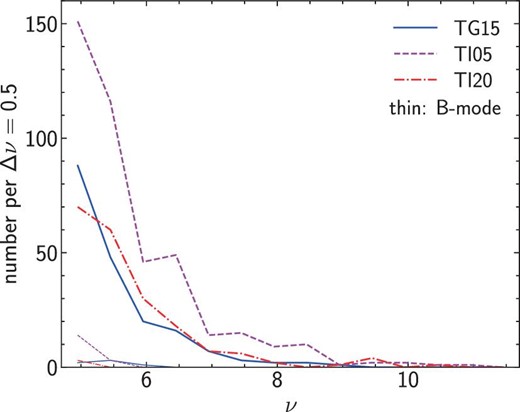
Distributions of the signal-to-noise ratio ν. The solid, dashed, and dash-dotted lines show the distributions for the TG15, TI05, TI20 set-ups summarized in table 1, respectively. The thin lines indicate the distributions of the signal-to-noise ratio ν from B-mode mass map peaks. (Color online)
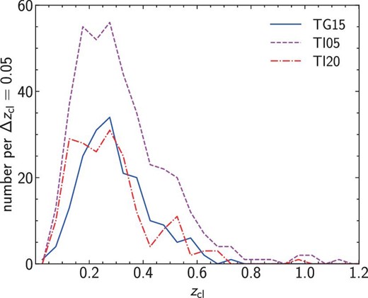
Similar to figure 3, but showing distributions of cluster redshift zcl. (Color online)
While weak lensing mass maps are constructed from E-mode shear, B-mode mass maps generated from B-mode shear provide an important means of checking the validity of the analysis (e.g., Utsumi et al. 2014). As a sanity check, we select mass map peaks from B-mode mass maps adopting the same signal-to-noise ratio threshold of ν ≥ 4.7. The distribution of B-mode mass map peaks is also shown in figure 3. In total there are 6, 17, and 3 B-mode mass map peaks with ν ≥ 4.7 for TG15, TI05, and TI20, respectively. We find that the numbers of B-mode mass map peaks are sufficiently small, ≲4%, compared with those of E-mode mass map peaks, which supports the high purity of our shear-selected cluster catalogs as estimated above.
In figure 5, we show distributions of the physical transverse distance between the shear-selected cluster and the primary matched optically selected cluster. We find that in most cases the distance is small, ≲0.3 h−1 Mpc. The mean distance is higher for TI20 than in the other set-ups, which can be understood by the conservative choice of Q(θ) to remove the small-scale information (see figure 1), which naturally leads to the degraded angular resolution of the resulting mass maps. For comparison, we also plot the distribution when using the random catalog mentioned above. Since the spatial distribution of the random catalog is not correlated with any optically selected clusters, the resulting distribution indicates that expected for matching by chance. We find that the distribution for the random catalog differs considerably from those for shear-selected clusters, supporting the high purity of our shear-selected cluster catalogs.
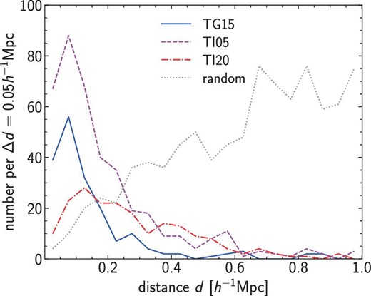
Similar to figure 3, but showing distributions of the physical transverse distance d between the shear-selected cluster and the primary matched optically selected cluster. The distribution of d for the case using the random catalog is also shown by the dotted line for reference. (Color online)
4.2 Weak lensing mass measurements
Following Miyazaki et al. (2018b), we derive the weak lensing masses of all the shear-selected clusters with redshift assignments by fitting their differential surface density profiles. We use the P-cut method (Oguri 2014; Medezinski et al. 2018) to securely select background galaxies for each shear-selected cluster, adopting zmin = zcl + 0.2 and Pth = 0.98 in equation (1). We derive the differential surface density profile ΔΣ(R) by fully taking account of the PDF of the photometric redshift of each galaxy (for a specific procedure, see, e.g., Medezinski et al. 2018), again adopting the dNNz photometric redshift measurements. For TG15, we derive differential surface density profiles in the range R = [0.3, 7] h−1 Mpc with a spacing of Δlog R = 0.09. The outer radius is chosen to be same as that used in Miyazaki et al. (2018b) and Chen et al. (2020), so that the mass bias derived in Chen et al. (2020) can be applied. We adopt a slightly larger inner boundary of R = 0.3 h−1 Mpc to mitigate the dilution effect by cluster member galaxies (Medezinski et al. 2018). For TI05 and TI20, we adopt a more conservative radius range of R = [0.3, 3] h−1 Mpc. In all cases, we consider the shape noise and ignore the cosmic shear error, again to follow the set-up assumed in Chen et al. (2020).
The differential surface density profiles are fitted with a Navarro–Frenk–White (NFW) profile (Navarro et al. 1997), which describes differential surface density profiles of clusters in numerical simulations reasonably well out to ∼10 times the virial radius (Oguri & Hamana 2011). We parameterize the NFW profile by M500c and c500c, which describe the mass and concentration parameter for the critical overdensity of 500. We restrict the range of the concentration parameter to 0.5 < c500c < 10 and derive both M500c and c500c from fitting to the observed differential surface density profile of each cluster. We show some examples of our tangential shear profile fitting in figure 6.
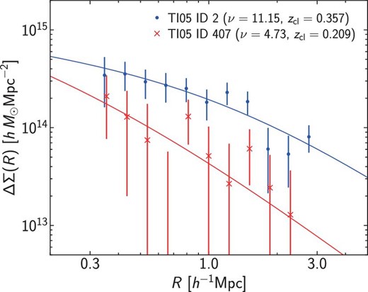
Examples of tangential shear profiles and fitting them with an NFW profile. We show examples for high and low signal-to-noise ratio ν from the TI05 catalog. Symbols with errors show the observed tangential shear profiles, and lines indicate best-fitting NFW profiles. The errors include only the shape noise. (Color online)
The derived weak lensing masses for the TG15, TI05, and TI20 catalogs as a function of the cluster redshift are shown in figure 7. The fitting results are also given in supplementary tables 1, 2, and 3. The increasing trend of weak lensing masses with increasing cluster redshift is theoretically expected for shear-selected clusters (see, e.g., Miyazaki et al. 2018b). The massive (M500c ∼ 1015 h−1 M⊙) cluster at zcl ∼ 0.18 is the well-known cluster Abell 1689 that has one of the largest Einstein radii known (e.g., Oguri & Blandford 2009). Our weak lensing mass estimation of Abell 1689 is consistent with more careful lensing mass estimates in the literature (e.g., Umetsu & Broadhurst 2008; Umetsu et al. 2015).
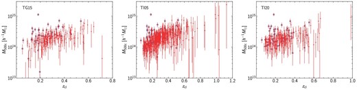
Weak lensing masses and redshifts of shear-selected clusters in the TG15 (left), TI05 (middle), and TI20 (right) catalogs. The red filled circles with 1 σ error bars show M500c derived from differential surface density profile fitting. The blue open circles indicate clusters that are matched with the CODEX catalog. (Color online)
In figure 7, we indicate clusters that are matched with the CODEX catalog. Only less than half of shear-selected clusters are matched with CODEX clusters (see also table 1), which is partly due to the shallow RASS X-ray data that is used to construct the CODEX catalog (Finoguenov et al. 2020). As a sanity check, we compare our weak lensing masses with X-ray luminosities provided by the CODEX catalog. Figure 8 shows the comparison of weak lensing masses with X-ray luminosities for the TI05 catalog. As expected, we find a good correlation between the masses and the X-ray luminosities. We note that deriving the underlying scaling relation requires the correction of selection biases of both the weak lensing selections in HSC-SSP and the X-ray selection in RASS. We plan to study the X-ray properties of these shear-selected clusters in more detail using the eROSITA Final Equatorial Depth Survey data that are much deeper than the RASS X-ray data, which will be reported in a separate paper (M. Ramos-Ceja et al. in preparation).
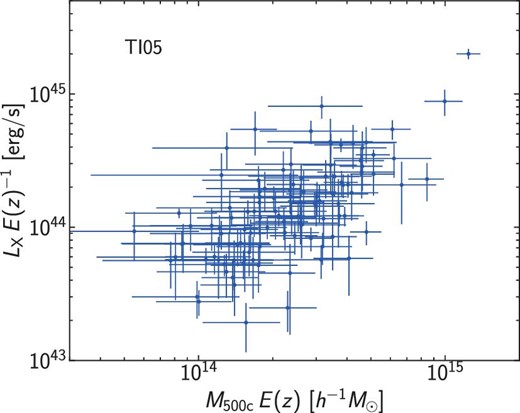
Weak lensing masses of shear-selected clusters in the TI05 catalog compared with X-ray luminosities of CODEX clusters that are matched with the shear-selected clusters, with the correction of the dimensionless Hubble parameter E(z). The X-ray luminosities are measured in the rest-frame 0.1–2.4 keV (Finoguenov et al. 2020). (Color online)
4.3 Effects of cluster member galaxies
Cluster member galaxies affect weak lensing measurements in two main ways. One is the enhancement of the number density of source galaxies due to the contribution of cluster member galaxies, which dilutes weak lensing signals. The other is the diminishment of the number density of source galaxies due to the obscuration of small galaxies by cluster member galaxies. The former effect can be mitigated by using only source galaxies located behind clusters for weak lensing measurements. Since these effects are more pronounced near centers of clusters, choosing the kernel function Q(θ) that has a smaller contribution from small θ can also mitigate the effects of cluster member galaxies. Here we check the number density profiles of our source galaxy samples around massive clusters to check how our weak lensing mass maps are affected by cluster member galaxies.
To reduce the statistical noise, we derive stacked number density profiles of source galaxies for samples of massive clusters. Purely optically selected clusters are not ideal for this purpose, because some optically selected clusters exhibit large off-centering up to ∼1 Mpc, which needs to be taken into account when interpreting observed stacked number density profiles. Thus, we adopt the CODEX cluster catalog and stack number density profiles around the X-ray centroids of CODEX clusters, because X-ray emission peaks are expected to be close to halo centers (e.g., Zhang et al. 2019).
Figure 9 shows stacked number density profiles for three CODEX cluster samples with different cluster redshifts. We also apply the richness cut for each cluster sample in order to select clusters with many cluster member galaxies, where the richness λ for CODEX clusters is measured using the redMaPPer algorithm (Rykoff et al. 2014). The richness threshold is determined so that a sufficient (≳50) number of clusters is included in each of the cluster subsamples. We show stacked number density profiles normalized by those computed with random source galaxy catalogs in order to highlight the effects of cluster member galaxies. We find a clear signature of the enhancement of number density profiles without any background galaxy selection. On the other hand, when source galaxies behind clusters are selected, we see decrements toward cluster centers due to the obscuration by cluster member galaxies (or magnification effects, see, e.g., Chiu et al. 2020). We find that the decrements are negligibly small at θ > 2′, suggesting that the TI20 catalog is little affected by cluster member galaxy obscurations. In contrast, the TG15 and TI05 catalogs are more or less affected by cluster member galaxies in the sense that the observed signal-to-noise ratios may be affected by the dilution or obscuration effect due to cluster member galaxies. Since cluster member galaxies do not contribute to the signal, the dilution effect enhances the noise and reduces the signal-to-noise ratio. The obscuration affects both the signal and the noise in a complicated manner. These effects may need to be taken into account when deriving an accurate selection function for shear-selected clusters in the TG15 and TI05 catalogs.
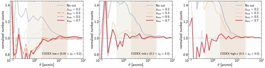
Stacked number density profiles of source galaxies around CODEX clusters. Here we show number density profiles relative to those from random source catalogs with their total numbers matched to the total numbers of source galaxy samples such that the normalized number density profile should be unity if there is no effect of cluster member galaxies. The different lines show the results for the different source galaxy samples summarized in table 1. From left to right, stacking is conducted around low-redshift clusters at 0.05 < zcl < 0.2 with richness λ > 25, intermediate redshift clusters at 0.2 < zcl < 0.3 with λ > 30, and high-redshift clusters at 0.3 < zcl < 0.4 with λ > 40. The results for background source galaxy samples satisfying zmin ≥ zcl + 0.1 for all the clusters are highlighted by thick lines. The narrow and wide shaded regions indicate the non-zero ranges of the kernel function Q(θ) for TI20 and TI05, respectively (see also figure 1). (Color online)
5 Conclusion
We have constructed shear-selected cluster catalogs by selecting peaks in weak lensing aperture mass maps covering ∼510 deg2 reconstructed by the HSC-SSP S19A shape catalog. Aperture mass maps are constructed using the truncated Gaussian filter (TG15) as well as the truncated isothermal filter with an inner boundary of |${0{^{\prime }_{.}}5}$| (TI05) and 2′ (TI20). For TI05 and TI20, we employ multiple source galaxy subsamples for which galaxies below redshift zmin are removed to improve the efficiency. With a signal-to-noise ratio threshold of 4.7, our shear-selected cluster catalogs contain 187, 418, and 200 clusters for the TG15, TI05, and TI20 set-ups, respectively. Cross matching with optically selected cluster catalogs suggests that the purity of the catalogs is high, more than 95% for TG15 and TI20 and more than 91% for TI05.
These catalogs represent by far the largest catalogs of shear-selected clusters to date with such a high signal-to-noise threshold, and will be useful for detailed studies of cluster astrophysics and cosmology. In this paper, we have demonstrated how the shape of the kernel function for constructing the aperture mass map can be optimized by adopting a flexible functional form of the filter function proposed by Schneider (1996). In particular, we have found that it is possible to choose the filter function such that it is almost free from effects of cluster member galaxies yet can select a sufficiently large number of clusters. Such a clean shear-selected cluster sample will be useful for obtaining accurate and robust constraints on cosmological parameters from the cluster abundance, in contrast to optically selected clusters for which constraining power appears to be limited by various systematic effects (Abbott et al. 2020). We will explore cosmological constraints with shear-selected clusters in a forthcoming paper.
Acknowledgements
We thank T. Hamana and K. Umetsu for useful discussions and comments. This work was supported in part by the World Premier International Research Center Initiative (WPI Initiative), MEXT, Japan, and JSPS KAKENHI Grant Nos. JP18K03693, JP20H00181, JP20H05856. This work was supported in part by Japan Science and Technology Agency (JST) CREST JPMHCR1414, and by JST AIP Acceleration Research Grant No. JP20317829, Japan.
The Hyper Suprime-Cam (HSC) collaboration includes the astronomical communities of Japan and Taiwan, and Princeton University. The HSC instrumentation and software were developed by the National Astronomical Observatory of Japan (NAOJ), the Kavli Institute for the Physics and Mathematics of the Universe (Kavli IPMU), the University of Tokyo, the High Energy Accelerator Research Organization (KEK), the Academia Sinica Institute for Astronomy and Astrophysics in Taiwan (ASIAA), and Princeton University. Funding was contributed by the FIRST program from the Japanese Cabinet Office, the Ministry of Education, Culture, Sports, Science and Technology (MEXT), the Japan Society for the Promotion of Science (JSPS), the Japan Science and Technology Agency (JST), the Toray Science Foundation, NAOJ, Kavli IPMU, KEK, ASIAA, and Princeton University.
This paper makes use of software developed for the Large Synoptic Survey Telescope. We thank the LSST Project for making their code available as free software at http://dm.lsst.org.
This paper is based on data collected at the Subaru Telescope and retrieved from the HSC data archive system, which is operated by the Subaru Telescope and Astronomy Data Center (ADC) at NAOJ. Data analysis was in part carried out with the cooperation of the Center for Computational Astrophysics (CfCA), NAOJ.
The Pan-STARRS1 Surveys (PS1) and the PS1 public science archive have been made possible through contributions by the Institute for Astronomy, the University of Hawaii, the Pan-STARRS Project Office, the Max Planck Society and its participating institutes, the Max Planck Institute for Astronomy, Heidelberg, and the Max Planck Institute for Extraterrestrial Physics, Garching, The Johns Hopkins University, Durham University, the University of Edinburgh, the Queen’s University Belfast, the Harvard-Smithsonian Center for Astrophysics, the Las Cumbres Observatory Global Telescope Network Incorporated, the National Central University of Taiwan, the Space Telescope Science Institute, the National Aeronautics and Space Administration under grant no. NNX08AR22G issued through the Planetary Science Division of the NASA Science Mission Directorate, the National Science Foundation grant no. AST-1238877, the University of Maryland, Eotvos Lorand University (ELTE), the Los Alamos National Laboratory, and the Gordon and Betty Moore Foundation.
Appendix. Optimization of the truncated isothermal filter
We optimize the parameters of the truncated isothermal filter as follows. For each source galaxy selection listed in table 1, we consider NFW halos located at z = zmin − 0.1 with varying halo mass as representative halos detected in mass maps with the source galaxy selection characterized by zmin. For each mass of the NFW halo, we vary ν1, ν2, and θR to search for the optimal set of parameters that maximizes νNFW, wLSS given by equation (A6). Since the combination of ν1θR determines the inner boundary of the filter (see subsection 3.3), in this paper we consider two cases, |$\nu _1\theta _R= {0{^{\prime }_{.}} 5}$| and 2′. The former is chosen to include the tangential shear at |$\theta \sim 1^{\prime }- {1{^{\prime }_{.}}5}$|, where the contribution to the signal is large. The latter removes a significant fraction of the inner part of the profile from the calculation, and hence is much less affected by various systematic effects as discussed in subsection 3.3 (see also subsection 4.3). First, we vary all three parameters with the constraint on ν1θR to find that νNFW, wLSS is generally maximized for ν2 ∼ 0.3–0.4. We thus fix ν2 = 0.36 throughout the paper and derive the optimal choice of ν1 and θR, as well as νNFW and νNFW, wLSS, as a function of the halo mass. We adopt values of ν1 and θR for the halo mass that yield νNFW ∼ 5, roughly corresponding to the threshold of constructing shear-selected clusters used in the literature. Parameters determined by this procedure for each ν1θR and the source galaxy selection are presented in table 1.
Footnotes
While the S20A version 2 CAMIRA cluster catalog, which includes photometry corrections to mitigate various photometry issues (Aihara et al. 2019), is currently available, in this paper we use the version 1 catalog that was the latest version when the shear-selected cluster catalogs were constructed.
