


Abstract
The barred spiral galaxy NGC 613 has a star-forming ring in the center, and near-infrared observations have previously shown that the star formation activity on the eastern and western sides of the ring is asymmetric. We examined the dynamics and physical state of the molecular gas in the ring using high-resolution (∼15 pc) 12CO(1–0), 12CO(3–2), and 13CO(1–0) observations with ALMA. Using a dendrogram, we identified 111 molecular clouds in the bar and ring, and found that the virial parameter (αvir) gradually decreases (αvir < 2) toward the confluence of the northern bar and eastern ring, while the virial parameter is large (αvir > 2) around the corresponding confluence in the western side of the ring. A non-LTE analysis using RADEX showed that the temperature and density of the molecular gas increase downstream of the eastern point of confluence, whereas they change irregularly on the western side. The star formation efficiency is (1.7 ± 0.2) × 10−8 yr−1 in the eastern side of the ring, which is substantially higher than the (0.9 ± 0.3) × 10−8 yr−1 for the western side of the ring. Position–velocity diagrams show that the relative velocity of the gas between the bar and the ring is ∼70 km s−1 in the east, while it reaches ∼170 km s−1 in the west. We suggest that the star formation activity in the central region of NGC 613 depends strongly on the relative velocity of the gas between the bar and the ring.
1 Introduction
In barred spiral galaxies, the non-axisymmetric bar potential causes large-scale streaming motions, efficiently transporting gas to the galactic center (e.g., Sellwood & Wilkinson 1993). This is consistent with the results of CO surveys, which showed that the central concentration of molecular gas is higher in barred spiral galaxies than in non-barred spiral galaxies (e.g., Sakamoto et al. 1999; Sheth et al. 2005; Kuno et al. 2007). This can result in starbursts with high star formation efficiency (SFE) in the center, as seen in NGC 253 (Daddi et al. 2010). However, recent molecular gas observations toward 80 galaxies showed that there is some variation in star formation activity in the central region of barred spiral galaxies (Muraoka et al. 2019). For example, NGC 4303 and NGC 4527, which are SAB types, have abundant gas but low SFE in the central region (Muraoka et al. 2019, Shibatsuka et al. 2003 and references therein; Devereux 1989; Young & Devereux 1991). What governs the SFE in the central region of barred spirals is not known, not least because it has not been investigated observationally on the scale of individual molecular clouds.
The difference in SFE in the bars compared to that in the arms is one example of where the gas dynamics is suspected to determine the SFE. Since both the bar and arm regions have an abundance of gas, star formation activity is expected to be high in both regions. However, observations of nearby barred spiral galaxies have shown that SFE in the bar regions is lower than in the arm regions (e.g., NGC 4303, Momose et al. 2010; NGC 1300, Maeda et al. 2020). In addition, several studies revealed that there are many gravitationally unbound molecular clouds in the bar regions (e.g., NGC 7479, Hüttemeister et al. 2000; NGC 3627, Morokuma-Matsui et al. 2015). The probable cause is that the collision velocity (i.e., velocity dispersion) between molecular clouds in the bar regions is higher than in the arm regions. This may prevent the molecular cloud cores in the bar regions from growing sufficiently large to form stars (e.g., Fujimoto et al. 2014; Yajima et al. 2019). Therefore, the different SFE in each region of the galaxy must be closely related to the dynamics of the gas as well as the physical state (e.g., size and mass) of the molecular cloud. Based on these studies, we speculate that the SFE in the central region of barred spiral galaxies is also regulated by the gas dynamics.
In order to investigate the influence of the gas dynamics on star formation in the central region of barred spiral galaxies, we focus on NGC 613, which is a relatively nearby (d = 17.5 Mpc; Tully 1988), strongly barred spiral galaxy [SB(rs)bc] (figure 1a). Table 1 summarizes the basic parameters of NGC 613. 12CO(1–0) observations with the Swedish–ESO submillimeter telescope (SEST) indicated that the central region of the galaxy is rich in molecular gas (Bajaja et al. 1995). Near-infrared observations of the central region (8″ × 8″) with the Very Large Telescope (VLT) revealed the morphology of a “star-forming ring” (250 pc < r < 340 pc) with active star formation (Böker et al. 2008). The Brγ observations exposed seven star-forming regions (so-called “hot spots”) along the ring (figure 1b), where Brγ is the hydrogen recombination line associated with O- or B-type stars. Furthermore, a “pearls on a string” scenario in the ring was suggested (Böker et al. 2008). In that scenario, gas from the bar enters the ring at the intersection of the offset ridges (dust lanes) of the bar and the inner Lindblad resonance (ILR), and the gas density gradually becomes high downstream in the ring. As a result, symmetric star formation activity is expected to occur in high-density regions downstream of these points of confluence. On the other hand, Falcón-Barroso et al. (2014) showed that the star formation rate (SFR) on the eastern side of the ring (0.10–0.13 M⊙ yr−1) is clearly higher than that on the western side (0.03–0.06 M⊙ yr−1). Note that the SFR in the circumnuclear disk (CND, r < 90 pc) is very low (0.02 M⊙ yr−1). The C2H(1–0, 3/2–1/2) line, which traces the gas irradiated by UV radiation from massive stars, is also remarkably strong on the eastern side of the ring (Miyamoto et al. 2017). This galaxy hosts an AGN with radio jets/outflow (Hummel et al. 1987). Recent papers on NGC 613 by Miyamoto et al. (2017, 2018) and Audibert et al. (2019) examined the properties of the gas in the central region using the Atacama Large Millimeter/submillimeter Array (ALMA) and found that star formation in the CND is suppressed by jets. Investigating the cause of the asymmetry of the star formation activity in the ring may give us clues to understand the reason for the diversity of SFE in the central region of barred spiral galaxies. Therefore, we observed the central region of NGC 613 using ALMA.
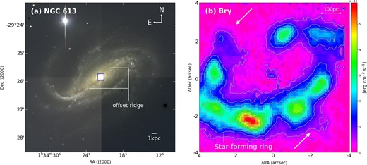
(a) VLT color-composite image of NGC 613, in blue (B band), green (V band), and red (R band). The blue square (14″ × 14″) is the region of CO lines observed by ALMA. (b) Brγ image in the central 8″ × 8″ region of NGC 613 with VLT (Böker et al. 2008). The contours are (0.1, 0.2, 0.3, 0.4, 0.5, 0.6, 0.7, 0.8, 0.9) × 5.8 × 10−14 erg cm−2 s−1 (maximum value). The white arrows indicate the gas flow from the bar (see figures 2 and 13 for details.). (Color online)
Parameters of NGC 613.
| Parameter | Value |
|---|---|
| RA (J2000.0)* | |${1^{\rm h}34^{\rm m}18{_{.}^{\rm s}}190}$| ‡ |
| Dec (J2000.0)* | |$-29^\circ {25^{\prime }6^{\prime \prime }.60}$| ‡ |
| Distance† | 17.5 Mpc |
| Position angle* | 118° ± 4° |
| Inclination angle* | 46° ± 1° |
| Systemic velocity (LSR)* | 1471 ± 3 km s−1 § |
This paper is structured as follows: In section 2, we describe 12CO(1–0) observations with ALMA. Section 3 explains the morphology and physical state of the molecular gas in NGC 613. In section 4, we investigate the gas dynamics, mainly from the bar to the ring (subsection 4.1), and discuss the relation between gas dynamics and star formation (subsection 4.2). Finally, we summarize our results in section 5.
2 Observations
We report the results of 12CO(1–0) (rest frequency: 115.271202 GHz) observations toward the galactic center of NGC 613 from a single pointing with ALMA as a Cycle 5 program (ID: 2017.1.01671.S, PI: Miyamoto). The observations were conducted in 2017 November and December. The phase reference center was adopted to be |$(\alpha _{\rm J2000.0}, \delta _{\rm J2000.0})=({1{\rm ^{h}}34{\rm ^{m}}18{_{.}^{\rm s}}190}, -29^\circ {25^{\prime }06.^{\prime \prime }60})$|, which is the position of the peak flux of the 350 GHz continuum (Miyamoto et al. 2017). The 12 m array (extended and compact) was used for the observations, with baseline lengths ranging from 15.1 m to 12.3 km. As a result, the maximum recoverable scale given by θMRS ∼ 0.6λ/Lmin is ∼21″ (1.8 kpc), which is larger than the region (∼14″) we are focusing on.
The calibration was performed with the Common Astronomy Software Application (CASA; McMullin et al. 2007), following the manuals provided by the ALMA observatory. The imaging was performed by Briggs weighting with a robustness parameter of 0.5 using the task tclean in CASA. Finally, the synthesized beam size was |${0{.^{\prime \prime }}18}\times {0{.^{\prime \prime}}14}$| (P.A. = 90°), corresponding to 15 × 12 pc at the distance to the galaxy. The velocity resolution was |$\rm 2.5\:$|km s−1. The data for 12CO(3–2) and 13CO(1–0) are from Miyamoto et al. (2017, 2018), respectively. The observational parameters for each emission line are summarized in table 2.
Summary of observation data.
| Frequency* | Eu/k† | Velocity resolution | Noise level | ||
|---|---|---|---|---|---|
| Transition | (GHz) | (K) | Beam size | (km s−1) | (Jy beam−1) |
| 12CO(1–0) | 115.271202 | 5.53 | |${0.^{\prime \prime }18} \times {0 .^{\prime \prime }14}$| (P.A. = 90°) | 2.5 | 5.09 × 10⁻⁴ |
| 12CO(3–2)‡ | 345.795990 | 33.19 | |${0 .^{\prime \prime }44} \times {0.^{\prime \prime }37}$| (P.A. = 45°) | 2.5 | 5.68 × 10⁻³ |
| 13CO(1–0)§ | 110.201354 | 5.29 | |${0.^{\prime \prime }42}\times {0.^{\prime \prime }35}$| (P.A. = −29°) | 10 | 2.91 × 10⁻⁴ |
Adopted from the NIST Recommended Rest Frequencies for Observed Interstellar Molecular Microwave Transitions 〈http://physics.nist.gov/cgi-bin/micro/table5/start.pl〉.
Leiden Atomic and Molecular Database.
Data from Miyamoto et al. (2017).
Data from Miyamoto et al. (2018).
3 Results
3.1 Molecular gas distribution and kinematics
We constructed moment maps of the 12CO(1–0) line emission in the central 1.2 kpc region of NGC 613. The velocity range used was 1250–1700 km s−1 and the intensity was clipped at 5σ (1σ = 5.09 × 10⁻⁴ Jy beam−1) for all moment maps. Figure 2a shows the distribution of the integrated intensity defined as I ≡ ΔvΣiIi at each position, where Δv is velocity resolution and Ii is the intensity in the ith channel with Δv. The structure of the northern and southern bar, the star-forming ring, and the nuclear spirals extending into the CND can be clearly seen. The integrated intensity in the ring (especially on the eastern and western sides) is stronger than in the bar, and a maximum value of Imax = 0.77 Jy beam−1 km s−1 is found in the CND. The peak intensity in the eastern and northwestern sides of the ring is higher than in the CND (figure 2b). This may be attributed to larger line widths in the CND due to the interactions with the jets and due to the fast galactic rotation (Miyamoto et al. 2017; Audibert et al. 2019). Furthermore, there are more clumpy intensity peaks on the eastern side of the ring than the western side. Miyamoto et al. (2018) also reported that the integrated intensities of CO isotopes of 13CO(1–0) and C18O(1–0), which can effectively trace higher number density regions than the optically thick 12CO, are weak in the southwestern side of the ring.
![Distributions of (a) integrated intensity (I ≡ ΔvΣiIi), (b) peak intensity, (c) mean velocity (〈v〉 ≡ ΣiIivi/ΣiIi), and (d) velocity dispersion [$\sigma _v\equiv \sqrt{\Sigma _iI_i(v_i-\langle v\rangle )^2/\Sigma _iI_i}$] of 12CO(1–0) clipped at 5σ in the central 14″ × 14″ region of NGC 613, where Δv is the velocity resolution and Ii and vi are the intensity and velocity in the ith channel with Δv, respectively. The structure of the northern and southern bars, the star-forming ring (250 pc < r < 340 pc) and the circumnuclear disk (CND, r < 90 pc) can be seen. The beam size of ${0.^{\prime \prime }18} \times {0.^{\prime \prime }14}$ is shown in the bottom left-hand corner of the velocity dispersion map. (Color online)](https://oup.silverchair-cdn.com/oup/backfile/Content_public/Journal/pasj/73/4/10.1093_pasj_psab060/2/m_psab060fig2.jpeg?Expires=1749563439&Signature=f84~9QYlISENDZnWNCDXykEb0-NpjZDJanWCxCo~gNENX9zNtKAOH3lnZFgrUVddWshLuQZUsEzRTpqMwchHQ03~1VRXGwLRGWaI1LyBlzGRHHSAF7d2j13tkSyLVidXhm029llqbZMIF3oRKxUbbmQ7bQvkcUnzHXk8gNGpQmOI3GYKRfrO6qrmuVoO0JKTKUJzYvpO-7lUUsSxXFozn~m7schSqv4zxj8bblovpa875UKo7pTKi4-ks5WFb7ogmGOPisyqAioDgBV4yc~eROPfZFjIfLSezP3u6aMebNiyDw01bVFoW7zO2J2FVXeNqzsaAdminQ71iyJ~oRa78Q__&Key-Pair-Id=APKAIE5G5CRDK6RD3PGA)
Distributions of (a) integrated intensity (I ≡ ΔvΣiIi), (b) peak intensity, (c) mean velocity (〈v〉 ≡ ΣiIivi/ΣiIi), and (d) velocity dispersion [|$\sigma _v\equiv \sqrt{\Sigma _iI_i(v_i-\langle v\rangle )^2/\Sigma _iI_i}$|] of 12CO(1–0) clipped at 5σ in the central 14″ × 14″ region of NGC 613, where Δv is the velocity resolution and Ii and vi are the intensity and velocity in the ith channel with Δv, respectively. The structure of the northern and southern bars, the star-forming ring (250 pc < r < 340 pc) and the circumnuclear disk (CND, r < 90 pc) can be seen. The beam size of |${0.^{\prime \prime }18} \times {0.^{\prime \prime }14}$| is shown in the bottom left-hand corner of the velocity dispersion map. (Color online)
Figure 2c shows the intensity-weighted mean velocity defined as 〈v〉 ≡ ΣiIivi/ΣiIi. The eastern side of the ring is blueshifted and the western side is redshifted with respect to the systemic velocity Vsys = 1471 km s−1, and the gas in the ring is generally moving in a counterclockwise circular motion. We note that the southwestern side of the ring, which is located near the minor axis (P.A. = 28°), shows a particularly strong redshift (i.e., deviating from circular motion). A more detailed discussion of the gas dynamics of the ring is given in sub-subsection 4.1.1.
A map of the line-of-sight velocity dispersion, defined as |$\sigma _v\equiv \sqrt{\Sigma _iI_i(v_i-\langle v\rangle )^2/\Sigma _iI_i}$|, is shown in figure 2d and shows enhancements due to the jet-driven outflows and due to cloud–cloud collisions (or turbulence). The velocity dispersion is ∼30 km s−1 on the eastern part of the ring, but has a very large value of ≥50 km s−1 in the western part. This trend is consistent with the results of the velocity dispersion of 12CO(3–2) (beam size |$\sim {0.^{\prime \prime }2}$|) found by Audibert et al. (2019). The asymmetric dynamics of the gas between the eastern and western parts of the ring is discussed in sub-subsection 4.1.2.
We examine the possibility that some of the flux of 12CO(1–0) could be lost in our 12 m array ALMA observations. To estimate the missing flux, we compared our data with the data of a single dish observation obtained by the CO Multi-line Imaging of Nearby Galaxies (COMING) project (Sorai et al. 2019). The ALMA data was convolved to the beam size (17″ × 17″) of the COMING data. Then, the velocity and spatial grids were regridded to 10 km s−1 and 6″, respectively, to match the COMING data. The region for comparison was the central 18″ × 18″ region, taking into account that the size of one pixel is 6″. The 12CO(1–0) line profile for ALMA and COMING is shown in figure 3. The total integrated intensity of ALMA and COMING were IALMA = 545.1 ± 2.7 K km s−1 and ICOMING = 532.4 ± 7.3 K km s−1, respectively. These values are consistent within the typical absolute flux error (|$5\%$| for ALMA in band 3 and |$20\%$| for the single dish), indicating that there is almost no missing flux.
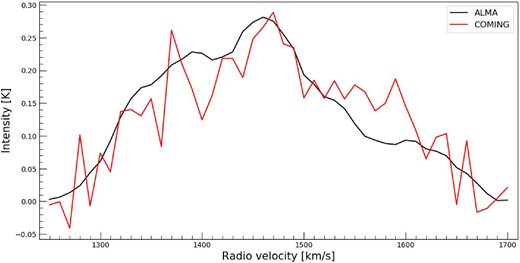
Spectral profiles of 12CO(1–0) observed by ALMA (black) and COMING (red), which is a single dish flux, in the central 18″ × 18″ region. (Color online)
3.2 Identification of molecular clouds
In order to investigate the differences in the properties of molecular clouds in each region, we identified molecular clouds using a dendrogram (Rosolowsky et al. 2008). Li et al. (2020) demonstrated that dendrograms are one of the best molecular cloud identification algorithms. The algorithm hierarchically separates the structure in the data cube using isocontours in intensity. The hierarchy is a collection of structures (trees) with the largest unit being the “trunk,” the next largest unit being “branches,” and the smallest unit (i.e., the maximum intensity contour) referred to as “leaves.” The trunk has no parent structure, and leaves have no sub-structure. The 12CO(1–0) datacube is of sufficiently high resolution (∼15 pc) to enable us to perform a well-resolved analysis across the typical diameter of a giant molecular cloud (GMC) (>20 pc; Sanders et al. 1985). In this study, we concentrate on the leaves because, in our data, these are the structures in the GMC with the highest gas density and therefore the regions most conducive to star formation. The minimum intensity threshold is 5σ (where σ is noise level) and the minimum intensity difference between adjacent structures is 2σ. The voxel detection threshold for the spatial scale and for velocity domain are three times the spatial resolution and twice the velocity channel width (5 km s−1), respectively. This allows us to exclude molecular clouds that are very large in size but have too small a velocity width (<1 km s−1) (and vice versa).
We identified 119 molecular clouds (figure 4a), of which 111 were in the bar and ring. We then derived the size R (the geometric mean radius calculated using the major and minor axis of the ellipse), line width dV, luminosity mass Mlum, and virial parameter αvir for each identified molecular cloud. The size and line width were corrected for spatial and velocity resolution, respectively. We also adopted |$R=(3.4/\sqrt{\pi })\, R_{\rm deconvolved}$| as the effective radius of a cloud (Solomon et al. 1987).
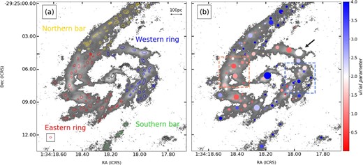
(a) 119 molecular clouds identified by dendrograms (ellipses) overlaid on the 12CO(1–0) integrated intensity map (gray scale). The colors of the molecular clouds indicate the regions of the eastern ring (red), the western ring (blue), the northern bar (yellow), and the southern bar (green); the rest are shown in black. The beam size is shown as a red ellipse in a black rectangle in the lower left-hand corner. (b) Virial parameter (color) for each molecular cloud, with the relative sizes of the circles indicating the relative luminosity mass. The red dots are molecular clouds with αvir < 2 and the blue dots are molecular clouds with αvir > 2. The dashed squares are the confluence regions described in sub-subsection 4.2.1. (Color online)
To examine the differences in the properties of the molecular clouds in more detail, we divided the region into an eastern ring, a western ring, a northern bar, and a southern bar, as shown in figure 4a. The average values of the molecular cloud parameters in each region are summarized in table 3.
Average value of the molecular cloud parameters in each region.
| R | dV | Mlum | |||
|---|---|---|---|---|---|
| Regions | (pc) | (km s−1) | (M⊙) | αvir | Number |
| Bar | 12.6 ± 1.0 | 13.4 ± 1.0 | (1.7 ± 0.4) × 105 | 3.7 ± 0.4 | 34 |
| Northern Bar | 12.0 ± 1.0 | 13.4 ± 1.1 | (1.7 ± 0.4) × 105 | 3.6 ± 0.4 | 30 |
| Southern Bar | 16.3 ± 3.7 | 14.5 ± 2.4 | (1.9 ± 1.2) × 105 | 4.7 ± 0.8 | 4 |
| Ring | 11.7 ± 0.6 | 13.2 ± 0.7 | (2.9 ± 0.4) × 105 | 2.4 ± 0.2 | 77 |
| Eastern Ring | 11.8 ± 0.7 | 12.5 ± 0.8 | (2.8 ± 0.5) × 105 | 2.1 ± 0.2 | 46 |
| Western Ring | 11.6 ± 0.9 | 14.2 ± 1.3 | (3.1 ± 0.8) × 105 | 2.8 ± 0.5 | 31 |
| All* | 11.9 ± 0.5 | 13.3 ± 0.6 | (2.6 ± 0.3) × 105 | 2.8 ± 0.2 | 111 |
Sum of bar and ring. The other eight are located in other regions.
3.2.1 Bar vs. ring
Histograms of R, dV, Mlum, and αvir of the identified molecular clouds in the bar (including the northern bar and southern bar) and ring (including the eastern ring and western ring) are shown in figure 5. There is no significant difference in the size and line width of the molecular clouds. The average mass of clouds in the ring is Mlum = (2.9 ± 0.4) × 105 M⊙, which is larger than the average mass of clouds [Mlum = (1.7 ± 0.4) × 105 M⊙] in the bar. This is consistent with the scenario in which the unbound gas supplied by the bar accumulates in the ring (i.e., bar-driven gas transport), leading to the growth of molecular clouds in the ring (e.g., Sakamoto et al. 1999; Nishiyama et al. 2001; König et al. 2016). Note, however, that we assume a constant XCO. The average values of the virial parameter are αvir = 3.7 ± 0.4 for bar and αvir = 2.4 ± 0.2 for ring, with the percentages of αvir < 2 being |$14.7\%$| and |$62.3\%$|, respectively. Furthermore, the p-value of the two-sample Kolmogorov–Smirnov (K–S) test for αvir of the bar and ring is 0.0021%, which is less than the significance level of |$5\%$| (indicators of significant difference). Thus, there is a clear difference in the physical states between the molecular clouds in the bar and those in the ring, with the ring having more gravitationally bound molecular clouds. This result is consistent with active star formation in the ring (figure 1b; Böker et al. 2008; Falcón-Barroso et al. 2014). In addition, the small number of gravitationally bound molecular clouds in the bar may be the reason for the generally low SFE. The molecular cloud with the largest line width and mass outside the CND is indicated by the arrows in figure 4b, where dV = 36.4 km s−1 and Mlum = 2.3 × 10⁶ M⊙ (αvir ∼ 2.0).
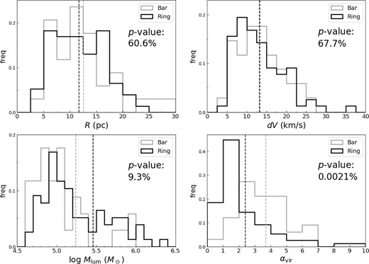
Normalized histograms of the radius R (top left), line width dV (top right), luminosity mass Mlum (bottom left), and virial parameter αvir (bottom right) of the molecular cloud identified in the bar and ring. The dashed lines in the figures show the average value of each. The p-value of the K–S test is also shown below the legend.
3.2.2 Eastern ring vs. western ring
The histogram of the same parameters as analyzed in sub-subsection 3.2.1, but compared between the eastern ring and western ring, is shown in figure 6. The eastern and western parts of the ring are separated by the galactic minor axis. The mean values of R, dV, Mlum, and αvir for the eastern ring and western ring are consistent within the margin of error (table 3). Furthermore, the results of the K–S test for each parameter are p–|${\rm value}>5\%$|, which means that the null hypothesis that the two samples come from the same distribution cannot be rejected (figure 6). Therefore, there is no statistical difference in these parameters of molecular clouds on the scale of eastern ring and western ring. However, we note that the fraction of molecular clouds with a large line width of dV ≥ 20 km s−1 is 25.8% for the western ring, and 8.7% for the eastern ring.
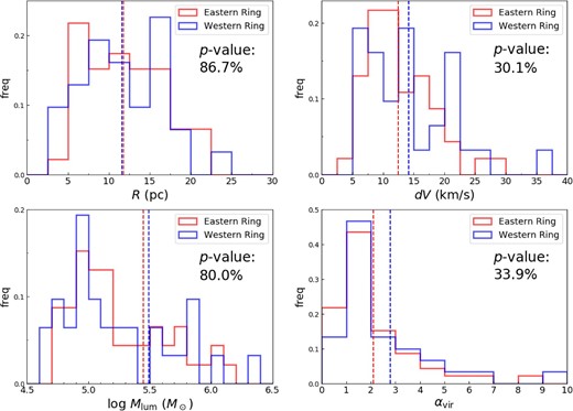
Normalized histograms of the radius R (top left), line width dV (top right), luminosity mass Mlum (bottom left), and virial parameter αvir (bottom right) of the molecular cloud identified in the eastern ring and western ring. The dashed lines in the figures show the average value of each. The p-value of the K–S test is also shown below the legend. (Color online)
3.3 Non-LTE analysis via RADEX
We used RADEX (van der Tak et al. 2007), a non-LTE code, for solving the statistical equilibrium radiative transfer in order to investigate the physical state of the gas. The kinetic temperature Tk and number density |$n_{\rm H_2}$| of the gas can be obtained by comparing the integrated intensity ratio of molecular emission lines calculated by RADEX with the observed data. The emission lines we used are 12CO(1–0), 12CO(3–2), and 13CO(1–0), which are convolved to a Gaussian beam with |${\rm FWHM}= {0.^{\prime \prime }72}$| (figures 7a and 7b). We define the integrated intensity ratios as |$R_{3/1}\equiv I_{^{12}\mbox{CO}(3-2)}/I_{^{12}\mbox{CO}(1-0)}$| and |$R_{13/12}\equiv I_{^{13}\mbox{CO}(1-0)}/I_{^{12}\mbox{CO}(1-0)}$| (figures 7c and 7d). R3/1 is relatively low (<0.5) in the bar and is in the range of 0.4–0.9 in the ring. R13/12 is also relatively low (<0.1) in the bar, and is higher in the eastern side (0.12–0.18) than in the western side (0.04–0.12) of the ring.
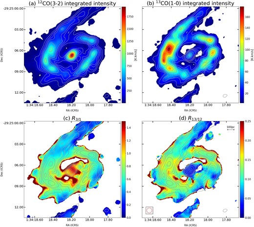
Distributions of (a) 12CO(3–2) integrated intensity, (b) 13CO(1–0) integrated intensity, (c) integrated intensity ratio of R3/1, and (d) integrated intensity ratio of R13/12. The integrated intensities of 12CO(3–2), 13CO(1–0), and 12CO(1–0) were clipped at 8σ (1σ = 0.14 K), 6σ (1σ = 0.045 K), and 8σ (1σ = 0.37 K), respectively, after convolving them with a Gaussian beam with |$\mbox{FWHM} = {0.^{\prime \prime }72}$|. The contours are 0.1, 0.2, 0.3, 0.4, 0.6, 0.8, and 0.95 of the 12CO(1–0) peak integrated intensity (1468.4 K km s−1). The high ratios around the edges of the R3/1 (>1.5) and R13/12 (>0.25) maps, i.e., outside of the lowest contour level, could be due to the large uncertainties of the integrated intensities and therefore are not included in the RADEX calculations. (Color online)
![Kinetic temperature Tk and number density $n_{\rm H_2}$ satisfied by R3/1 (black) and R13/12 (red) via RADEX calculations, where dV = 13.3 km s−1, L = 23.8 pc, [12CO]/[H2] = 8.0 × 10⁻⁵, and [12CO]/[13CO] = 80 are assumed. The contours are R3/1 = 0.2, 0.4, 0.6, 0.8, 0.9 and R13/12 = 0.04, 0.06, 0.08, 0.10, 0.12, 0.14. (Color online)](https://oup.silverchair-cdn.com/oup/backfile/Content_public/Journal/pasj/73/4/10.1093_pasj_psab060/2/m_psab060fig8.jpeg?Expires=1749563439&Signature=fRv7wiKgUPGq9JHqIY40nzMMiHY1IwEoRB-aUMFsF~vUioSTlLt~qEpK9kvYeHzhBas5PGh8VGxRByYtSp90kRq23N77GfDBSLOWUMj07qk11-5W~9YfQVrVCf1sKi-RWoobMyoft5z~VKDrxTmFLAU1PBTccOVIRImAVeBXIDyxe-MCy23aiU5Vkp0J391uWNHE9m2ByexrQK7QfJgbvIMhm3MqdpMk5aNXJDz0THAzdH1ZrqSUulmBy2zhB10Y55rU7lQpeR92vvePuc7pzLMR9qSXOZILtjQEFQmlyk9yAUsawtejJxJAREnrQUS6tlLc2q1fouW8E3BT8O7XJA__&Key-Pair-Id=APKAIE5G5CRDK6RD3PGA)
Kinetic temperature Tk and number density |$n_{\rm H_2}$| satisfied by R3/1 (black) and R13/12 (red) via RADEX calculations, where dV = 13.3 km s−1, L = 23.8 pc, [12CO]/[H2] = 8.0 × 10⁻⁵, and [12CO]/[13CO] = 80 are assumed. The contours are R3/1 = 0.2, 0.4, 0.6, 0.8, 0.9 and R13/12 = 0.04, 0.06, 0.08, 0.10, 0.12, 0.14. (Color online)
The distribution of Tk and |$n_{\rm H_2}$| derived from the RADEX calculations is shown in figure 9. The contours in the left-hand panel of figure 9 show the 100 GHz continuum. Miyamoto et al. (2017) reported that the continuum emission in the ring can be dominated by free-free emission due to massive stars and that the nuclear jets extend north- and southward from the center. The contours in the right-hand panel of figure 9 show the velocity dispersion of 12CO(1–0). The temperature, Tk, is in the range of 30–60 K in the bar, but in the range of 40–170 K in the ring. The density, |$n_{\rm H_2}=10^{2.6-3.8}\:$|cm−3 in the ring is higher than the density of |$n_{\rm H_2}=10^{2.3-2.6}\:$|cm−3 in the bar. From Spot B1 to Spot 2 via Spots B2, 1a, and 1b, we can find that the density increases sequentially (|$n_{\rm H_2}=10^{2.3-3.0}\:$|cm−3). We note that the density increases to |$n_{\rm H_2}\sim 10^{2.8}\:$|cm−3, although there is no increase in temperature (Tk ∼ 40 K) toward Spot 1b. The temperature rises from Tk ∼ 40 K (|$n_{\rm H_2}\sim 10^{2.8}\:$|cm−3) to Tk ∼ 60 K (|$n_{\rm H_2}\sim 10^{3.0}\:$|cm−3) between Spot 1b and Spot 2, where the intensity of Brγ and the 100 GHz continuum become strong. One of the causes of the increase in temperature at Spot 2 could be the effect of UV radiation from massive stars formed from rapidly growing molecular clouds. Downstream of Spot 2 (Spot 3 and Spot 4), the temperature and density are almost constant at Tk ∼ 70 K and |$n_{\rm H_2}\sim 10^{3.0}\:$|cm−3. In Spot 5, the temperature and density are very high (Tk ∼ 160 K and |$n_{\rm H_2}\sim 10^{3.5}\:$|cm−3). Note that SiO, a strong shock tracer, has been detected near Spot 5, at the end of the jets (Miyamoto et al. 2017). There is also a density gradient of |$n_{\rm H_2}=10^{2.3-3.0}\:$|cm−3 from Spot B3 to Spot 8 via Spots B3, 6, and 7, but there is a rapid temperature increase of Tk ∼ 140 K (|$n_{\rm H_2}\sim 10^{2.8}\:$|cm−3) in Spot 6. Downstream of Spot 6 (Spot 7 and Spot 8), the temperature is almost constant at Tk ∼ 60 K and the density increases from |$n_{\rm H_2}\sim 10^{2.8}\:$|cm−3 to |$n_{\rm H_2}\sim 10^{3.0}\:$|cm−3. The values of R3/1, R13/12, Tk, and |$n_{\rm H_2}$| for each spot are summarized in table 4. The errors for Tk and |$n_{\rm H_2}$| are determined from the 1σ errors of R3/1 and R13/12. The SFR and SFE are explained in sub-subsection 4.2.2.
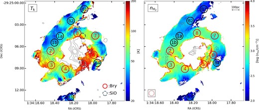
Maps of the kinetic temperature Tk (left) and number density |$n_{\rm H_2}$| (right) obtained from RADEX calculations and maps of R3/1 and R13/12. The contours of the left-hand panel are 4σ, 6σ, 8σ, 10σ (1σ = 28 μJy beam−1) of the 100 GHz continuum, and the contours of the right-hand panel are 20, 30, 40 km s−1 of the velocity dispersion of 12CO(1–0). The seven red circles indicate hotspots of Brγ with a diameter of 1″ shown in figure 1b (Falcón-Barroso et al. 2014). The black circle is the same size area of the bar and ring for comparison. The dashed circle is the area where SiO was detected (Miyamoto et al. 2017). (Color online)
Average physical parameters of the gas at each spot.
| Tk* | log |$n_{\rm H_2}$|* | |$\Sigma _{\rm H_2}$|* | SFR† | SFE | |||
|---|---|---|---|---|---|---|---|
| Position | R3/1 | R13/12 | [K] | [cm−3] | [M⊙ pc−2] | [M⊙ yr−1] | [×10−8 yr−1] |
| Spot 1a | 0.53 ± 0.01 | 0.11 ± 0.005 | |$43^{+6}_{-4}$| | |$2.65^{+0.03}_{-0.02}$| | |$(5.2^{+0.4}_{-0.2})\times 10^2$| | — | — |
| Spot 1b | 0.65 ± 0.01 | 0.14 ± 0.003 | |$42^{+3}_{-3}$| | |$2.84^{+0.01}_{-0.02}$| | |$(8.1^{+0.1}_{-0.4})\times 10^2$| | — | — |
| Spot 2 | 0.75 ± 0.01 | 0.15 ± 0.004 | |$58^{+6}_{-4}$| | |$3.00^{+0.02}_{-0.03}$| | |$(1.2^{+0.1}_{-0.1})\times 10^3$| | 0.13 | 2.0 |
| Spot 3 | 0.73 ± 0.01 | 0.12 ± 0.004 | |$76^{+8}_{-7}$| | |$2.96^{+0.03}_{-0.03}$| | |$(1.1^{+0.1}_{-0.1})\times 10^3$| | 0.10 | 1.7 |
| Spot 4 | 0.77 ± 0.02 | 0.13 ± 0.008 | |$73^{+14}_{-12}$| | |$3.05^{+0.08}_{-0.06}$| | |$(1.3^{+0.3}_{-0.2})\times 10^3$| | 0.10 | 1.4 |
| Spot 5 | 0.84 ± 0.02 | 0.09 ± 0.005 | |$163^{+15}_{-14}$| | |$3.45^{+0.11}_{-0.10}$| | |$(3.3^{+1.0}_{-0.7})\times 10^3$| | 0.08 | 0.4 |
| Spot 6 | 0.68 ± 0.01 | 0.08 ± 0.004 | |$137^{+22}_{-17}$| | |$2.83^{+0.04}_{-0.03}$| | |$(7.9^{+0.8}_{-0.5})\times 10^2$| | 0.06 | 1.4 |
| Spot 7 | 0.67 ± 0.01 | 0.12 ± 0.004 | |$57^{+6}_{-6}$| | |$2.84 ^{+0.02}_{-0.03}$| | |$(8.1^{+0.4}_{-0.5})\times 10^2$| | 0.03 | 0.7 |
| Spot 8 | 0.73 ± 0.04 | 0.14 ± 0.013 | |$61^{+19}_{-14}$| | |$2.97^{+0.08}_{-0.08}$| | |$(1.1^{+0.2}_{-0.2})\times 10^3$| | 0.04 | 0.7 |
| Spot B1 | 0.34 ± 0.01 | 0.06 ± 0.007 | |$60^{+34}_{-17}$| | |$2.28 ^{+0.07}_{-0.08}$| | |$(2.2^{+0.4}_{-0.4})\times 10^2$| | — | — |
| Spot B2 | 0.48 ± 0.01 | 0.10 ± 0.006 | |$42^{+8}_{-6}$| | |$2.59 ^{+0.03}_{-0.04}$| | |$(4.5^{+0.3}_{-0.4})\times 10^2$| | — | — |
| Spot B3 | 0.29 ± 0.03 | 0.07 ± 0.014 | |$38^{+48}_{-15}$| | |$2.30^{+0.11}_{-0.16}$| | |$(2.3^{+0.7}_{-0.7})\times 10^2$| | — | — |
| Spot B4 | 0.47 ± 0.02 | 0.09 ± 0.008 | |$54^{+22}_{-13}$| | |$2.51^{+0.05}_{-0.06}$| | |$(3.8^{+0.5}_{-0.5})\times 10^2$| | — | — |
Value assuming [12CO]/[13CO] = 80. Errors are determined from the 1σ errors of R3/1 and R13/12
Falcón-Barroso et al. (2014)
In this paper, we do not derive Tk and |$n_{\rm H_2}$| in the CND with RADEX. However, the high R3/1 ∼ 1.3 and low R13/12 ∼ 0.04 in the CND suggest that the physical state of the gas is different from that in the bar and ring. In Miyamoto et al. (2017), non-LTE analysis using HCN, HCO+, and CS emission lines revealed that the temperature in the CND is very high (Tk > 300 K).
4 Discussion
4.1 Gas dynamics
4.1.1 Comparison with a model of circular motion
We compared the observed dynamics of the gas in the ring with a tilted ring model generated by |$^{\rm 3D}\mathit {Barolo}$| (Di Teodoro & Fraternali 2015). |$^{\rm 3D}\mathit {Barolo}$|, which is a powerful fitting routine for a thin regularly rotating disk, fits a tilted-ring model to a 3D datacube of an emission line using parameters such as position angle (φ), inclination angle (i), systemic velocity (Vsys), rotational velocity (Vrot), and velocity dispersion (σv). The data cube of 12CO(1–0) above 5σ was used for the analysis. The central region of NGC 613 (r ≤ 5″) was divided into 50 annuli, with a thickness of z = 150 pc and a width of |$\Delta r={0.^{\prime \prime }1}\sim \theta _{\rm maj}/2$| (θmaj is the major axis of the synthesized beam); beyond this radius, the influence of the bar is too strong to obtain reliable results assuming circular motion. For the dynamical center of the annuli (x0, y0), φ, i, and Vsys, we used the values in table 1 (Miyamoto et al. 2017). The free parameters were Vrot and σv, and radial velocity was set to Vrad = 0 km s−1 to assume circular motion.
Figures 10a and 10b show the velocity field of the observed data and the model, respectively. The residual velocity field obtained by subtracting the model from the observed data is shown in figure 10c. The ring matches the circular motion well, except on the western side. The residual in the western side of the ring is Vres ∼ +130 km s−1, which represents gas associated with the strong redshifted component. The residual component fades rapidly but smoothly from the bar to the ring: gas is inflowing from the bar and settling promptly on to the circular motion of ring. This trend is consistent with the results of the analysis using 12CO(3–2) by Audibert et al. (2019). Furthermore, this region has a large velocity dispersion (figure 2d) and is coincident with the region of strong [Fe ii] (1.6 μm) radiation induced by a fast shock (Böker et al. 2008).
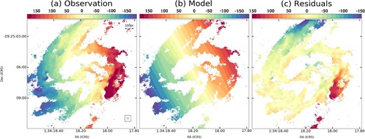
(a) Velocity field of 12CO(1–0) clipped at 5σ and based on Vsys = 1471 km s−1. (b) Velocity field of the model derived by |$^{\rm 3D}\mathit {Barolo}$|. (c) Residuals subtracting the velocity field of the model from the observed data. (Color online)
4.1.2 Non-circular motion in the confluence region
Using position–velocity (P–V) diagrams, we investigated the strong non-circular motion on the western side of the ring revealed in sub-subsection 4.1.1. To capture the flow of gas from the bar to the ring, we made P–V diagrams for the eastern and western sides of the ring symmetrically (figure 11). We placed four slits of length 3″ on either side, and label them Ea, Eb, Ec, Ed, and Wa, Wb, Wc, Wd, from north to south. The black contours are the intensities of the 12CO(1–0) emission line and the red contours are the intensities from the |$^{\rm 3D}\mathit {Barolo}$| model, indicating that the gas is in circular motion if the respective contours overlap. In the eastern side of the ring, near Ea–Eb, the gas in the bar merges with the gas with the circular motion in the ring, and the relative velocity between the bar and ring is Vrel ∼ 70 km s−1. The virial parameter of the molecular clouds transitions from αvir > 2 to αvir < 2 beyond this point of confluence (figure 4b). Near Ec, the gas becomes almost a single component, transitioning to circular motion. On the western side of the ring, near Wa, the velocity difference between the gas in the bar and the gas with circular motion in the ring is Vrel ∼ 170 km s−1, which is much larger than the corresponding offset on the eastern side of the ring. The two gas components create a bridge structure at Wb and interact with each other. Further downstream, near Wc, the velocity dispersion of the gas is larger than that predicted by the model, and there are many molecular clouds that exhibit αvir > 2 in this confluence region (figure 4b), implying that the gas is dissipating. Therefore, the western side of the ring likely hosts more violent collisions between the bar and the ring than the eastern side. The collisions on the western side of the ring are the cause of the large residual velocity (figure 10c) and the large velocity dispersion (figure 2d). Taking into account that the temperature is Tk ∼ 60–80 K even in the case of Spot 2–Spot 4, where the heating due to star formation is dominant, the rapid temperature rise (Tk ∼ 140 K) in Spot 6 is most likely due to either shock heating by violent collisions in the region of confluence, or jet heating. The latter seems less likely when looking at the density map (figure 9), which shows a gap between the high-density region caused by the jet-compression (the SiO detection site) and the linear high-density region (|$n_{\rm H_2}>10^{3.5}\:$|cm−3) to the west and north of this. The compression, heating, and high velocity dispersion in Spot 6 is, therefore, more likely to have been created by violent collisions in the region of confluence. The detection of a strong |$\rm H_2$| line (2.1 μm) in the southwestern part of the ring is consistent with our interpretation (Böker et al. 2008). Furthermore, H i observations may be of interest because collisions may have increased the atomic gas in this region. The gas components of the ring before inflow in both the eastern and western sides show systemic velocities, but the deviation from the systemic velocity of the gas in the bar is |Vnorthern bar − Vsys| ∼ 90 km s−1 and |Vsouthern bar − Vsys| ∼ 180 km s−1 in Ea and Wa, respectively. In other words, the reason for the different relative gas velocities between the bar and the ring in the respective confluence regions is attributed to the inflowing gas in the bar.
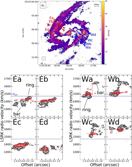
P–V diagrams of the confluence regions between the bar and the ring on the eastern side (bottom left) and western side (bottom right) of the ring along the slit shown above the velocity dispersion (top center) of 12CO(1–0). The length of the slit is 3″. The black contours are the observed data and the red contours are the model with |$^{\rm 3D}\mathit {Barolo}$|. The contour levels are 4σ, 5σ, 8σ, 10σ, 15σ, 20σ, 30σ. The blue dashed line is the systemic velocity. (Color online)
4.2 Star formation activity in the ring
4.2.1 Physical state of the gas in the confluence regions
The reason for the similarity in the physical parameters of the molecular clouds between the eastern ring and western ring, as seen in sub-subsection 3.2.2, could be due to the fact that the molecular clouds are growing and dissipating along the ring by the gas inflow and that molecular clouds in various states are mixed when comparing in the ring scale (including the confluence region and downstream). Therefore, we review the physical state of the molecular cloud, focusing on the confluence region from the bar in the east and west of the ring, where asymmetric gas dynamics were found. The histograms of R, dV, Mlum, and αvir of the molecular clouds in the areas indicated by the dashed square in figure 4b (i.e., the confluence regions of the bar and the ring) are shown in figure 12, and the average values are listed in table 5. There is little difference in the size of the molecular clouds. While no molecular clouds exceeding dV = 20 km s−1 are detected in the eastern confluence region, the fraction of molecular clouds exceeding dV = 20 km s−1 is as high as |$29.4\%$| in the western confluence region. In terms of mass, the average value for the eastern confluence region is Mlum = (3.4 ± 0.9) × 105 M⊙, which is larger than Mlum = (2.1 ± 0.5) × 105 M⊙ on the western confluence region. The fraction of molecular clouds with αvir < 2 is |$92.3\%$| in the eastern confluence region, while the fraction of molecular clouds with αvir < 2 is relatively low (|$41.1\%$|) in the western confluence region. Furthermore, the p-value of the K–S test for αvir is |$0.080\%$|, which is a statistically significant difference. Therefore, in the eastern confluence region, the majority of the molecular clouds are gravitationally bound and are likely to result in star formation, while in the western confluence region the line width in the molecular clouds is large and the mass is small, resulting in fewer gravitationally bound molecular clouds. This result is consistent with more active star formation on the eastern side of the ring than on the western side (Falcón-Barroso et al. 2014).
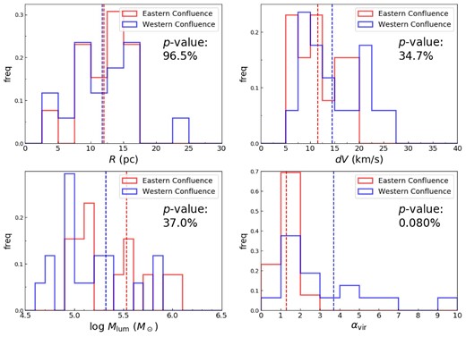
Normalized histograms of the radius R (top left), line width dV (top right), luminosity mass Mlum (bottom left), and virial parameter αvir (bottom right) of the molecular cloud identified in the eastern confluence region and western confluence region. The dashed lines in the figures show the average value of each. The p-value of the K–S test is also shown below the legend. (Color online)
Average value of the molecular cloud parameters in confluence regions.
| R | dV | Mlum | |||
|---|---|---|---|---|---|
| Regions | (pc) | (km s−1) | (M⊙) | αvir | Number |
| Eastern confluence | 12.0 ± 1.0 | 11.6 ± 1.3 | (3.4 ± 0.9) × 105 | 1.3 ± 0.1 | 13 |
| Western confluence | 11.8 ± 1.3 | 14.5 ± 1.4 | (2.1 ± 0.5) × 105 | 3.7 ± 0.7 | 17 |
| R | dV | Mlum | |||
|---|---|---|---|---|---|
| Regions | (pc) | (km s−1) | (M⊙) | αvir | Number |
| Eastern confluence | 12.0 ± 1.0 | 11.6 ± 1.3 | (3.4 ± 0.9) × 105 | 1.3 ± 0.1 | 13 |
| Western confluence | 11.8 ± 1.3 | 14.5 ± 1.4 | (2.1 ± 0.5) × 105 | 3.7 ± 0.7 | 17 |
4.2.2 SFE in the confluence regions
Falcón-Barroso et al. (2014) derived the SFR at each hot spot in the ring of NGC 613 from the intensity of Brγ accounting for the effect of extinction. Using the SFR and molecular mass derived from the column density (|$\Sigma _{\rm H_2}=n_{\rm H_2}\times L$|), we measure SFE at each spot (table 4). The SFE at Spot 2 is the highest, with a value of 2.0 × 10⁻⁸ yr−1, and the lowest value is 0.4 × 10⁻⁸ yr−1 at Spot 5. The average value on the eastern side of the ring (Spot 2–Spot 4) is (1.7 ± 0.2) × 10−8 yr−1, while on the western side (Spot 6–Spot 8) it is (0.9 ± 0.3) × 10−8 yr−1, about half as high as on the eastern side. Miyamoto et al. (2017) showed that heating of the gas by the jet suppressed star formation in the CND, resulting in lower SFE. Similarly, at Spot 5, where the effect of the jet is suggested by the detection of SiO, the gas is heated (|$T_{\rm k}\sim 163^{+15}_{-14}\:$|K), which may be the reason for the lowest SFE.
4.2.3 Relation between gas dynamics and star formation
We discuss the relation between the properties of molecular clouds that we have studied above and the star formation activity in the ring. On the eastern side of the ring, gas flows from the northern bar with a relatively small relative velocity (Vrel ∼ 70 km s−1) around Spot 1a (figure 11), and signs of active star formation are seen in Spot 2 (table 4). Based on the rotation curve of the gas in the ring derived from Miyamoto et al. (2017), the timescale required to move from Spot 1b to Spot 2 is approximately 0.8 Myr. The free-fall time for a molecular cloud is estimated to be |$t_{\rm ff}\sim 4.0\times 10^7(1/n_{\rm H_2})^{1/2}\sim 1.5\:$|Myr, using |$n_{\rm H_2}(=\!10^{2.8}\:\mbox{cm}^{-3})$| in Spot 1b. However, considering that the density is averaged over the beam size (|${0.^{\prime \prime }72}\times {0.^{\prime \prime }72}$|) and is much higher on the molecular cloud core scale, where star formation occurs, the value of tff is an upper limit. Therefore, it is probable that the gas in the bar enters the ring and becomes denser, forming stars immediately. By contrast, on the western side of the ring, the gas flows from the southern bar with the large relative velocity of Vrel ∼ 170 km s−1 (i.e., large velocity dispersion) around Spot 6 (figure 11), and star formation is inactive compared to the eastern side of the ring (table 4). Such a large velocity gradient may lead to a rapid destruction of molecules. We stress, however, that this velocity does not represent the shock speed of a standing transverse shock. The region is more likely dominated by supersonic turbulence, in particular shear and vortical flows containing much weaker, highly oblique shocks that are less likely to destroy molecules. Simulations show that the CO formation time in typical molecular clouds is of the order of a Myr (Glover et al. 2010), so that even if a fraction of the molecules is destroyed, molecules could reform on timescales comparable to the cooling and dissipation time (see below).
How long is the turbulence induced by the violent collisions in the region of confluence expected to persist downstream? We compare dissipation timescales to the dynamical time of the gas in the ring. The turbulent dissipation timescale (eddy turnover time) of a GMC (McKee & Ostriker 2007) is estimated to be tdiss ∼ 0.5(d/σv) ∼ 1.9 Myr, where the diameter (d = 23.5 pc) and velocity dispersion (σv = 6.2 km s−1) are taken from the mean values of molecular clouds in the confluence region (western dashed square in figure 4b). This is consistent with the timescale (∼2.2 Myr) required to move from Spot 6 to Spot 7. The post-shock cooling time (tcool) of two merging streams of gas separated by a shock of speed is calculated by |$t_{\rm cool}\sim 2.2\times 10^{-16}(\sigma _{\rm sh}^2/n_{\rm H_2} \Lambda )\sim 5.5\:$|Myr (e.g., Dyson & Williams 1997), where the velocity dispersion (σsh = 50 km s−1) and number density (|$n_{\rm H_2}=10^{3.0}\:$|cm−3) are values in the shock region and Λ (=10−22 erg s−1 cm3) is the cooling rate. Thus the cooling time is even larger than the eddy turnover time, which means that radiative cooling is not an important mode of dissipation and strong turbulence can persist a substantial distance downstream of the region of confluence.
The presence of a molecular cloud with the largest line width (dV = 36.4 km s−1) near Spot 7 in the ring (see the arrow in figure 4b) implies that the turbulence caused by the collisions has not yet subsided or that more intense collisions may have occurred in the past. That molecular cloud has the largest mass (Mlum = 2.3 × 10⁶ M⊙) in the ring and αvir ∼ 2.0, which may trigger a starburst in the near future. Thus, we propose that the SFE on the western side of the ring (Spot 6–Spot 8) is significantly smaller than that on the eastern side of the ring (Spot 2–Spot 4) due to the strong turbulence generated at the confluence of bar and ring, which persists downstream into the ring.
From these results, we conclude that the relative velocity of the gas between the bar and the ring strongly influences the star formation activity in the galactic center. A schematic diagram of the process of star formation in the central region of NGC 613 is shown in figure 13. In the case of small relative velocity of the gas between the bar and the ring (eastern side), the molecular clouds become dense and gravitationally bound downstream of the point of confluence, which induces star formation and leads to the pearls on a string scenario (in which stars are sequentially formed downstream of the point of confluence). Contrarily, in the case of large relative velocity (western side), violent collision shocks would heat up the molecular clouds and cause the clouds to dissipate and increase the velocity dispersion, thereby suppressing star formation even downstream. We suggest that the diversity of star formation activity in the central region of barred spiral galaxies may be due to such large variations in the gas dynamics. However, the reason for differences in the way the gas falls from the bar to the ring (relative velocity) is not clear. One possibility may be a difference in the angle between the inflowing gas from the bar and the ring. The same analysis performed for galaxies with different bar strengths can clarify the differences in the effect of each galaxy on star formation.
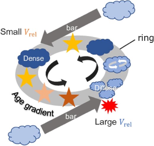
Schematic diagram of the star formation activity in the central region of NGC 613. On the left is the case where the velocity difference of the gas between the bar and the ring is small, leading to sequential star formation (pearls on a string scenario). On the right is the case where the velocity difference is large, leading to suppressed or delayed star formation. (Color online)
4.2.4 Comparison with other studies
Based on spatially- and velocity-wise well-resolved observations of Galactic molecular clouds, cloud–cloud collisions (CCC) are thought to play an important role in massive star formation (e.g., Torii et al. 2011; Fukui et al. 2014). In these studies, the typical collision velocity at which star formation is induced is Vrel ∼ 20 km s−1, much smaller than the values found in our study (e.g., eastern side of the ring: Vrel ∼ 70 km s−1). The result of a more recent paper reported that young massive clusters are formed by CCC with Vrel ∼ 100 km s−1 between galaxies (Tsuge et al. 2021), which is consistent with our results showing that molecular clouds grow and star formation is caused around Spot 2. While collision velocities of up to perhaps 100 km s−1 may trigger star formation, our results from the western ring of NGC 613 also indicate that too high a collision velocity (Vrel ∼ 170 km s−1) can suppress star formation. Furthermore, Yajima et al. (2019) reported that when inter-cloud velocity dispersion is moderate (ΔV/sin i ≤ 100 km s−1), |$n_{\rm H_2}$| increases with increasing velocity dispersion, but when it is too large (ΔV/sin i ≥ 100 km s−1), |$n_{\rm H_2}$| decreases with increasing velocity dispersion. On the other hand, Maeda et al. (2021) showed that the massive star formation in the bar and bar-end depends not only on the CCC speed but also on other parameters, including mass and density of the GMC. We conclude that investigating collision velocities and the physical state of the gas in the center of nearby barred spiral galaxies, where more intense phenomena are expected to occur than in other regions of the galaxy, will be very useful in understanding the diversity in the rates of molecular cloud growth and in the SFE.
5 Summary
In this study, we investigated the physical state and dynamics of the molecular gas in the central region of NGC 613 using high-resolution CO observations with ALMA. We discovered a connection between features in the gas dynamics and star formation activity in the star-forming ring. The main conclusions are summarized as follows:
12CO(1–0) emission was detected in the bar, star-forming ring, and CND. The integrated intensity in the ring (especially eastern and western sides) is stronger than in the bar.
111 molecular clouds were identified in the bar and ring using a dendrogram. For the bar, the percentage of the virial parameter αvir > 2 is |$85.3\%$|. The virial parameter decreases from αvir > 2 to αvir < 2 from the northern bar to the eastern side of the ring, whereas many molecular clouds remain αvir > 2 from the southern bar to the western side of the ring. The result of the K–S test for the virial parameter in each confluence region is |$p{\rm -value}=0.080\%$|, indicating there is a statistical difference.
The temperature and density of the gas in the bar and ring were estimated from a non-LTE analysis with RADEX using the integrated intensity ratios of 12CO(1–0), 12CO(3–2), and 13CO(1–0). From the northern bar to the eastern side of the ring, there is a clear density gradient of |$n_{\rm H_2}=10^{2.3-3.0}\:$|cm−3 and a temperature increases from ∼40 K to ∼70 K, where the high-temperature region corresponds to the star-forming region. There is a rapid temperature increase of Tk ∼ 140 K at the point of confluence in the western side of the ring.
A comparison with the velocity field of a tilted disc model assuming circular motion generated by |$^{\rm 3D}\mathit {Barolo}$| revealed a large inward non-circular motion (Vres ∼ +130 km s−1) in the western confluence region of the ring.
The P–V diagrams in the respective confluence regions of the bar and the ring show that gas on the north side of the bar flows into the eastern side of the ring at a relative velocity of Vrel ∼ 70 km s−1, while gas on the south side of the bar flows into the western side of the ring at Vrel ∼ 170 km s−1.
Using SFR estimated from Brγ and the density derived by RADEX, the SFE was found to be (1.7 ± 0.2) × 10−8 yr−1 on the eastern side of the ring and (0.9 ± 0.3) × 10−8 yr−1 on the western side of the ring.
Based on these results, we conclude that the relative velocity of the gas between the bar and the ring has a significant impact on the star formation activity in the central region of the barred spiral galaxy; in the case of a small relative velocity of the gas between the bar and the ring, massive stars are sequentially formed from the confluence (pearls on a string), whereas in the case of a large relative velocity, the molecular clouds dissipate and the velocity dispersion increases, leading to a suppression of star formation. Such gas dynamics may explain the diversity of star formation in the central region of barred spiral galaxies.
Acknowledgements
This paper makes use of the following Atacama Large Millimeter/submillimeter Arra data: ADS/JAO.ALMA#2013.1.01329.S, #2015.1.01487.S, and #2017.1.01671.S. ALMA is a partnership of European Southern Observatory (representing its member states), National Science Foundation (USA) and National Institutes of Natural Sciences (Japan), together with National Research Council (Canada), Ministry of Science and Technology and Academia Sinica Institute of Astronomy and Astrophysics (Taiwan), and Korea Astronomy and Space Science Institute (Republic of Korea), in cooperation with the Republic of Chile. The Joint ALMA Observatory is operated by ESO, AUI/National Radio Astronomy Observatory and National Astronomical Observatory of Japan. This publication made use of data from COMING, CO Multi-line Imaging of Nearby Galaxies, a legacy project of the Nobeyama 45-m radio telescope. Based on data obtained from the ESO Science Archive Facility under request number #FORS1.2001-12-19T00:32:08.634, #FORS1.2001-12-19T00:34:12.021 and #FORS1.2001-12-19T00:36:15.217. We thank J. Falcón-Barroso for providing us the data with Very Large Telescope (figure 1b). This work was supported by Ministry of Education, Culture, Sports, Science and Technology Leading Initiative for Excellent Young Researchers (HJH02007).
