


Abstract
We performed follow-up photometric observations on exoplanetary system HAT-P-37 from 2011 February to 2019 September. The nine new transit light curves of the R and V bands are presented in this work. Based on the new light curves and published literature data, the physical and orbital parameters of HAT-P-37 are refined. In addition, mid-transit times are obtained to update the linear ephemeris, Tc[0] = 2456478.57916 ± 0.00077 [BJDTDB], P = 2.7974415 ± 0.0000025 d. Moreover, the transit timing variations (TTVs) have an rms of 57 s and there is no significant TTV signal. According to dynamic analysis, we excluded the possibility of perturbers with a mass larger than 200M⊕, when located in 1 : 3, 1 : 2, 2 : 3 (interior) or 3 : 2, 2 : 1, 5 : 2, 3 : 1 (exterior) orbital resonance, respectively.
1 Introduction
The first exoplanet discovered in 1995 (Mayor & Queloz 1995) opened up a colorful world to human beings. In the past two decades, more than 4300 exoplanets have been discovered, which gives us opportunities to gain insight into the formation and evolution of exoplanetary systems.1
There are two main techniques to search for exoplanets: radial velocity (RV) and transits. The RV method detects exoplanets by measuring Doppler red (blue) shift of the spectral line of a star (Mayor & Queloz 1995), and transit photometry discovers exoplanets through the change in the brightness (flux) of the host star (Charbonneau et al. 2000; Henry et al. 2000). Before the launch of the Kepler space telescope (Borucki et al. 2010), the RV method contributed |$80\%$| of the discovery of exoplanets. As the data of Kepler were released, more exoplanets were discovered though the transit method. To date, ∼ 3200 transiting exoplanets have been found. As the Transiting Exoplanet Survey Satellite (TESS) (Ricker et al. 2015) mission goes on, over 10 thousand transiting exoplanets are to be found, confirmed, and characterized. An abundant sample of exoplanets will help us further understand the formation and evolution of exoplanetary systems.
Photometric follow-up observations for exoplanetary systems are required for the characterization of confirmed exoplanets. Although thousands of exoplanets have been discovered, most of them lack adequate follow-up observations. Photometric follow-up observations can refine the physical and orbital parameters of exoplanetary systems. Moreover, based on the accumulated mid-transit times, transit timing variation (TTV) studies can be carried out (e.g., Agol et al. 2005; Holman & Murray 2005), which offers the possibility of detecting dynamically near-by perturbers (e.g., Kepler-9; Hinse et al. 2010; Wang et al. 2018). Moreover, the trend in TTVs is able to reveal the evolution of the planetary system, like WASP-12. The apparent shortening of the orbital period indicates that the planet WASP-12b is at the end of its life (Bailey & Goodman 2019; Maciejewski et al. 2016a; Patra et al. 2017; Yee et al. 2020).
The planetary nature of HAT-P-37 was unveiled by Bakos et al. (2012). It comprises a solar-like star and a typical hot Jupiter with a period of about 2.8 d. The host star has an effective temperature of Teff = 5570 ± 100 K, a mass of M* = 0.929 ± 0.043 M⊙, and a radius of |$\, R_{\rm *}= 0.877^{+0.059}_{-0.044} \, R$|⊙. Bakos et al. (2012) reported the mass and radius of this planet are 1.169 ± 0.103 MJ and 1.178 ± 0.077 RJ, respectively. Bakos et al. (2012) presented three follow-up light curves and RVs from Fred Lawrence Whipple Observatory (FLWO) 1.5-m/Tillinghast Re-flector Echelle Spectrograph (TRES) observations . Maciejewski et al. (2016b) has observed another four transit light curves, and found the results of observations were consistent with Bakos et al. (2012) within 1σ. Turner et al. (2017) refined the system parameters by fitting five transits including two new transits from their work and three from Bakos et al. (2012).
In this work, we simultaneously modeled 18 light curves and one set of RV curves from literature (Bakos et al. 2012). Those 18 light curves include nine light curves reported in this paper and nine light curves from the literature. A global fit was conducted to improve the precision of orbital parameters, physical parameters, and mid-transit times. Based on mid-transit times, we updated the ephemeris equation. Moreover, the TTVs of this system were studied to analyze the orbital stability and limit of the upper mass on potential perturbers.
The organization of this paper is as follows. In section 2, observations and data reduction are described in detail. The fitting of light curves and RVs is presented in section 3. The discussion of the fitting results, TTVs, and potential perturbers for this system are in section 4. A brief summary is presented in the final section.
2 Observations and data reduction
2.1 Photometric observations
With the Weihai Observatory 1.0 m telescope of Shandong University (WHOT), we carried out nine photometric observations for the HAT-P-37 from 2013 to 2019. The WHOT is equipped with a 2 K × 2 K CCD. A field of view (FOV) of 12′ × 12′ is provided. More information on instruments can be found in Hu et al. (2014).
A standard Johnson–Cousins V filter was used for all photometric observations except observations of 2018 November 11 and 2019 September 09. For those two observations, an R filter was used. During observations, time in UTC was synchronized with GPS and was recorded in the headers of images. The detailed observation information is presented in table 1.
Log of observations.
| Date | Time | Band | Number of | Exposure | Airmass | Moon | Angular | PNR* |
|---|---|---|---|---|---|---|---|---|
| (UTC) | (UTC) | exposures | time (s) | phase | distance (°) | (% minute−1) | ||
| 2013 Sep. 18 | 12:15:09–15:48:34 | V | 240 | 40 | 1.06–1.60 | 0.98 | 131.41 | 0.65 |
| 2013 Oct. 12 | 12:01:44–15:11:30 | V | 223 | 40 | 1.10–1.71 | 0.07 | 68.87 | 0.41 |
| 2013 Oct. 30 | 11:06:08–13:28:10 | V | 140 | 50 | 1.19–1.75 | 0.18 | 65.28 | 0.62 |
| 2015 Jul. 13 | 12:32:58–16:29:30 | V | 190 | 60 | 1.19–1.03–1.05 | 0.07 | 110.22 | 0.45 |
| 2015 Sep. 21 | 10:34:47–15:19:22 | V | 228 | 60 | 1.03–1.51 | 0.51 | 143.57 | 0.56 |
| 2017 Jun. 14 | 16:26:44–19:41:00 | V | 177 | 60 | 1.04–1.03–1.16 | 0.77 | 111.97 | 1.18 |
| 2017 Jun. 28 | 16:01:00–19:41:00 | V | 177 | 60 | 1.03–1.26 | 0.27 | 44.40 | 0.93 |
| 2018 Nov. 11 | 10:17:14–13:12:25 | R | 410 | 20 | 1.19–1.97 | 0.15 | 129.89 | 0.37 |
| 2019 Sep. 09 | 12:34:27–16:29:41 | R | 192 | 60 | 1.05–1.62 | 0.81 | 139.20 | 0.55 |
Photometric noise rate, calculated as rms|$/\sqrt{\Gamma }$|, where rms is the scatter in the light curve residuals and Γ is the median number of cycles (exposure time and any dead time such as read-out time) per minute.
2.2 Data reduction
C-Munipack (Breus 2017) was used for the reduction of images.2 Bias and flat correction were carried out on all images. After aperture photometry, the selection of the comparison star and photometric aperture was optimized to ensure that light curves with high quality can be derived. Based on the technique described in Eastman et al. (2010), we have converted the timestamps from UTC to BJDTDB.
3 Light curve analysis
To update the system parameters, a global fitting was carried out on 18 light curves and RVs using EXOFASTv2 (Eastman 2017; Eastman et al. 2019).3 The 18 light curves include nine new light curves from this work, three light curves from Bakos et al. (2012), four light curves from Maciejewski et al. (2016b), and two light curves from Turner et al. (2017). The RVs are from Bakos et al. (2012).
EXOFASTv2 is an exoplanet-fitting package that can deal with light curves, RVs, and astrometric data sets of multiple exoplanets from multiple observatories (Eastman et al. 2019). It can simultaneously fit transit data and RVs. The uncertainties in the parameters were calculated through a differential evolution Markov chain Monte Carlo (DE-MCMC) algorithm (Ter Braak 2006).
We imposed priors, including an orbital period (P) of 2.7973600 ± 0.000007 d, an epoch of the transit center of Tc = 2455642.14318 ± 0.00029, a stellar effective temperature (Teff) of 5500 ± 100 K, metallicity ([Fe/H]) of 0.03 ± 0.1, and a surface gravity (log g) of 4.520 ± 0.05 (cgs). All the above priors are from Bakos et al. (2012). Moreover, a Gaia parallax (Gaia Collaboration 2018) of 2.61 ± 0.05 mas, adjusted according to the suggestion of Stassun and Torres (2018), and an upper limit of V-band extinction (0.12648) was used to constrain the radius of the host better. Based on the flux of broadband photometry, an Spectral Energy Distribution (SED) + MESA Isochrones and Stellar Tracks (MIST) (Choi et al. 2016; Dotter 2016) fit was employed to derived parameters of the host star HAT-P-37.
According to the prior values, the AMOEBA algorithm (Nelder & Mead 1965) minimized χ2 with a step length of 10000, which means the local minimum is determined. Then, the most extensive matching model is determined and DE-MCMC is performed to estimate the uncertainties. The criteria of convergence for chains of all parameters are the following: (1) the Gelman–Rubin statistic is less than 1.01; (2) the independent draws are made more than 1000 times. Markov chains are considered to be well-mixed once they satisfy these two criteria for six consecutive times. The obtained system parameters and the uncertainties of parameters are listed in table 2. The best-fitting model for light curves and RVs are shown in figures 1, 2, and 3. The resulting mid-transit times are shown in table 3.
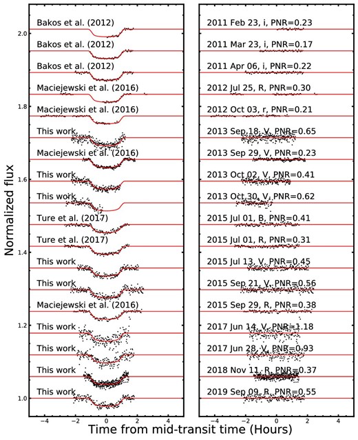
All light curves including nine new transit data from this work, three transit data from Bakos et al. (2012), four transit data from Maciejewski et al. (2016b), and two transit data from Turner et al. (2017) for HAT-P-37b. In the left-hand panel, red solid lines represent best-fitting models, and the photometric noise rate (PNR) in units of hundredths per minute is plotted on the right. (Color online)
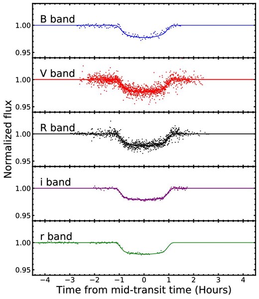
The best-fitting model to all light curves is plotted as the solid line in green (B band), purple (V band), black (R band), red (i band), and blue (r band). (Color online)
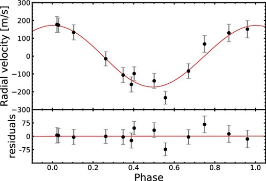
FLWO 1.5-m/TRES RV measurements of HAT-P-37 from Bakos et al. (2012). The best fit is plotted as solid red line. The O − C residuals are displayed on the bottom panel, which has an rms scatter σ = 36.5 ms−1. (Color online)
System parameters for HAT-P-37.
| Parameter | Units | This work | B12† | σ‡ | M16§ | σ | T17‖‖ | σ |
|---|---|---|---|---|---|---|---|---|
| Stellar parameters | ||||||||
| M* | Mass (M⊙) | 0.942|$_{-0.040}^{+0.035}$| | 0.929 ± 0.043 | 0.22 | — | — | — | — |
| R* | Radius (R⊙) | 0.8639|$_{-0.0069}^{+0.0070}$| | 0.877|$_{-0.044}^{+0.059}$| | 0.29 | 0.887|$_{-0.028}^{+0.033}$| | 0.45 | — | — |
| L* | Luminosity (L⊙) | 0.609|$_{-0.091}^{+0.015}$| | 0.62|$_{-0.09}^{+0.11}$| | 0.12 | — | — | — | — |
| ρ* (ρ⊙) | Density (cgs) | 2.058|$_{-0.094}^{+0.086}$| | — | — | 1.33|$_{-0.11}^{+0.13}$| | 4.54 | — | — |
| log g | Surface gravity (cgs) | 4.539|$_{-0.019}^{+0.016}$| | 4.52 ± 0.05 | 0.36 | 4.510|$_{-0.038}^{+0.046}$| | 0.58 | — | — |
| Teff | Effective temperature (K) | 5487|$_{-49}^{+33}$| | 5500 ± 100 | 0.11 | — | — | — | — |
| [Fe|$/$|H] | Metallicity (dex) | 0.18 ± 0.12 | +0.03 ± 0.10 | 1.01 | — | — | — | — |
| Age | Age (Gyr) | 2.7|$_{-1.9}^{+3.2}$| | 3.6|$_{-2.2}^{+4.1}$| | 0.23 | — | — | — | — |
| dpc | Distance (pc) | 395.1 ± 2.7 | 411 ± 26 | 0.61 | — | — | — | — |
| Planetary parameters | ||||||||
| P | Period (d) | 2.7974415 ± 0.0000025 | 2.797436 ± 0.000007 | 0.74 | 2.7974471 ± 0.0000011 | 2.07 | 2.79744149 ± 0.00000083 | 0.01 |
| Rp | Radius (RJ) | 1.152 ± 0.012 | 1.178 ± 0.077 | 0.33 | 1.231|$_{-0.043}^{+0.048}$| | 1.77 | 1.16 ± 0.06 | 0.13 |
| Mp | Mass (MJ) | 1.17 ± 0.12 | 1.169 ± 0.103 | 0.01 | 1.19 ± 0.11 | 0.12 | 1.17 ± 0.10 | 0.00 |
| a | Semi-major axis (au) | 0.03810|$_{-0.00054}^{+0.00047}$| | 0.0379 ± 0.0006 | 0.25 | 0.03791 ± 0.00059 | 0.24 | 0.0394 ± 0.0029 | 0.44 |
| e | Eccentricity | 0.020|$_{-0.014}^{+0.018}$| | 0.058 ± 0.038 | 0.90 | — | — | — | — |
| ϖ* | Argument of periastron (°) | 160 ± 110 | — | — | — | — | — | — |
| Teq | Equilibrium temperature (K) | 1259 ± 12 | 1271 ± 47 | 0.25 | — | — | 1250 ± 22 | 0.24 |
| ρp | Density (cgs) | 0.95 ± 0.10 | 0.89 ± 0.19 | 0.28 | 0.846 |$_{-0.089}^{+0.095}$| | 0.75 | 0.93 ± 0.17 | 0.10 |
| log gp | Surface gravity (d) | 3.341|$_{-0.049}^{+0.043}$| | 3.32 ± 0.07 | 0.25 | — | — | 3.369 ± 0.088 | 0.29 |
| θ | Safronov number | 0.0825 |$_{-0.0083}^{+0.0080}$| | 0.081 ± 0.009 | 0.12 | — | — | 0.085 ± 0.012 | 0.17 |
| 〈F〉 | Incident flux (109 erg s−1 cm−2) | 0.570 ± 0.021 | 0.589|$_{-0.075}^{+0.102}$| | 0.24 | — | — | — | — |
| RV parameters | ||||||||
| κ | RV semi-amplitude (m s−1) | 176|$_{-18}^{+17}$| | 177.7 ± 14.8 | 0.08 | 180 ± 16 | 0.17 | — | — |
| TP[BJDTDB2450000 +] | Time of periastron | 5709.72|$_{-0.81}^{+0.83}$| | — | — | — | — | — | — |
| e cosω* | |$-0.002_{-0.021}^{+0.016}$| | −0.017 ± 0.039 | 0.43 | — | — | — | — | |
| e sin ω* | 0.002|$_{-0.013}^{+0.018}$| | 0.007 ± 0.060 | 0.08 | — | — | — | — | |
| Mpsini | Minimum mass (MJ) | 1.17 ± 0.12 | 1.169 ± 0.103 | 0.01 | — | — | — | — |
| Mp/M* | Mass ratio | 0.00119 ± 0.00012 | — | — | — | — | — | — |
| Primary transit parameters | ||||||||
| Tc [BJDTDB2450000 +] | Time of transit | 6478.57916 ± 0.00077 | 5642.14318 ± 0.00029 | — | 5642.143820 ± 0.000156 | — | 5616.96710 ± 0.00028 | — |
| i | Inclination (°) | 87.04 ± 0.17 | 86.9|$_{-0.5}^{+0.4}$| | 0.32 | 86.67 |$_{-0.33}^{+0.40}$| | 0.85 | 87.4 ± 0.82 | 0.43 |
| Rp/R* | Radius of planet in stellar radii | 0.13702|$_{-0.00081}^{+0.00079}$| | 0.1378 ± 0.0030 | 0.25 | 0.1394|$_{-0.0020}^{+0.0017}$| | 1.11 | 0.1361 ± 0.0028‡‡ | 0.32 |
| a/R* | Semi-major axis in stellar radii | 9.48|$_{-0.15}^{+0.13}$| | 9.32|$_{-0.57}^{+0.42}$| | 0.36 | 9.19|$_{-0.25}^{+0.31}$| | 0.84 | 9.68 ± 0.52 | 0.37 |
| δ | Transit depth (fraction) | 0.01877 ± 0.00022 | — | — | — | — | — | — |
| τ | Ingress/egress transit duration (d) | 0.01484 |$_{-0.00056}^{+0.00057}$| | — | — | — | — | — | — |
| T14 | Total transit duration (d) | 0.09652 |$_{-0.00055}^{+0.00056}$| | 0.0971 ± 0.0015 | 0.36 | — | — | — | — |
| TFWHM | FWHM♯ duration (d) | 0.08168 ± 0.00037 | — | — | — | — | — | — |
| b | Transit impact parameter | 0.488|$_{-0.028}^{+0.025}$| | 0.505|$_{-0.0628}^{+0.041}$| | 0.25 | 0.533|$_{-0.065}^{+0.055}$| | 0.65 | — | — |
| PT | A priori non-grazing transit prob | 0.0913|$_{-0.0021}^{+0.0026}$| | — | — | — | — | — | — |
| PT, G | A priori transit prob | 0.1203|$_{-0.0028}^{+0.0034}$| | — | — | — | — | — | — |
| μ1 (linear) | linear limb-darkening coeff | —** | — | — | — | — | — | — |
| μ2 (quadratic) | quadratic limb-darkening coeff | —†† | — | — | — | — | — | — |
| Occultation parameters | ||||||||
| bs | Eclipse impact parameter | 0.490 ± 0.022 | — | — | — | — | — | — |
| τs | Ingress/egress eclipse duration (d) | 0.01493|$_{-0.00052}^{+0.00062}$| | — | — | — | — | — | — |
| TS,FWHM | FWHM duration (d) | 0.0819|$_{-0.0015}^{+0.0020}$| | — | — | — | — | — | |
| TS,14 | Total eclipse duration (d) | 0.0969|$_{-0.0018}^{+0.0024}$| | 0.0981 ± 0.0083 | 0.14 | — | — | — | — |
| TS [BJDTDB2450000 +] | Time of eclipse | 5710.678|$_{-0.038}^{+0.028}$| | 5643.512 ± 0.070 | — | — | — | — | — |
| PS | A priori non-grazing eclipse prob | 0.0908 ± 0.0014 | — | — | — | — | — | — |
| PS,G | A priori eclipse prob | 0.1197 |$_{-0.0019}^{+0.0020}$| | — | — | — | — | — | — |
B12 represents Bakos et al. (2012).
σ represents agreement between this work with previous work.
M16 represents Maciejewski et al. (2016b).
T17 represents Turner et al. (2017).
FWHM stands for full width at half maxima
For B band, μ1 = 0.751± 0.046. For R band, μ1 = 0.442 |$_{-0.023}^{+0.024}$|. For Sloan i band, μ1 = 0.351 ± 0.026. For r band, μ1 = 0.410 ± 0.042. For V band, μ1 = 0.543 |$_{-0.022}^{+0.023}$|
For B band, μ2 = 0.064 ± 0.049. For R band, μ2 = 0.250 ± 0.022. For Sloan i band, μ2 = 0.241 ± 0.027. For r band, μ2 = 0.187 ± 0.047. For V band, μ2 = 0.205 |$_{-0.021}^{+0.020}$|.
The RP/R* of 0.1361 ± 0.0028 is the R band.
Mid-transit times for HAT-P-37.
| Epoch | Telescope | Tc | σ | O − C | Data source |
|---|---|---|---|---|---|
| (BJDTDB) | (d) | (d) | |||
| −308 | FLWO 1.2 m | 2455616.96721 | 0.00060 | 0.00004 | Bakos et al. (2012) |
| −298 | FLWO 1.2 m | 2455644.94117 | 0.00023 | −0.00042 | Bakos et al. (2012) |
| −293 | FLWO 1.2 m | 2455658.92842 | 0.00029 | −0.00038 | Bakos et al. (2012) |
| −123 | CAO 1.23 m | 2456134.49411 | 0.00050 | 0.00026 | Maciejewski et al. (2016b) |
| −98 | Cassini 1.52 m | 2456204.43100 | 0.00049 | 0.00111 | Maciejewski et al. (2016b) |
| 27 | WHOT 1.0 m | 2456554.10966 | 0.00093 | −0.00042 | This work |
| 31 | Piwnice 0.6 m | 2456565.30121 | 0.00026 | 0.00137 | Maciejewski et al. (2016b) |
| 32 | WHOT 1.0 m | 2456568.09693 | 0.00061 | −0.00036 | This work |
| 42 | WHOT 1.0 m | 2456596.07120 | 0.00120 | −0.00050 | This work |
| 260 | Kuiper 1.55 m | 2457205.91408 | 0.00064 | 0.00013 | Turner et al. (2017) |
| 260 | Kuiper 1.55 m | 2457205.91304 | 0.00042 | −0.00091 | Turner et al. (2017) |
| 264 | WHOT 1.0 m | 2457217.10261 | 0.00056 | −0.00110 | This work |
| 289 | WHOT 1.0 m | 2457287.03974 | 0.00067 | −0.00001 | This work |
| 292 | OGS 1.0 m | 2457295.43143 | 0.00053 | −0.00065 | Maciejewski et al. (2016b) |
| 515 | WHOT 1.0 m | 2457919.26120 | 0.00140 | −0.00033 | This work |
| 520 | WHOT 1.0 m | 2457933.24960 | 0.00130 | 0.00086 | This work |
| 699 | WHOT 1.0 m | 2458433.99031 | 0.00045 | −0.00046 | This work |
| 807 | WHOT 1.0 m | 2458736.11486 | 0.00071 | 0.00041 | This work |
4 Discussion and analysis
4.1 System parameters
With the global fit using EXOFASTv2, the physical and orbital parameters of HAT-P-37 were updated. For comparison, all parameters of HAT-P-37 from our work and the previous works are listed in table 2.
Most of the parameters derived from our fit are consistent with previous works (Bakos et al. 2012; Maciejewski et al. 2016b; Turner et al. 2017). According to table 2, all important parameters are improved by the global fitting, except metallicity, planetary mass, RV semi-amplitude, and minimum mass of the planet. Since the same RVs were used, there is no doubt that all Doppler velocimetric properties show great agreement with the previous works (Bakos et al. 2012; Maciejewski et al. 2016b; Turner et al. 2017). Table 2 shows that the RV parameters obtained from this work are consistent within 0.43σ compared with the previous works. Since we used the same stellar spectroscopic parameters as the previous works, our determinations are in agreement with the results reported in the literature. Since we have collected more extensive data of transit light curves, we obtained more precise transit ephemeris.
4.2 The refined ephemeris
Based on the updated linear ephemeris, the observed minus calculated mid-transit times is derived (see figure 4), and it has an rms of residuals of 57 s. We employed the generalized Lomb–Scargle (GLS) algorithm (Zechmeister & Küurster 2009) to investigate whether there is a periodic signal in the O − C (see figure 5). Moreover, the power thresholds for false alarm probability (FAP) levels of |$10\%$|, |$1\%$|, and |$0.1\%$| were derived. The highest peak of the periodogram does not exceed the threshold of |$\mbox{FAP} = 0.1\%$|, which indicates that there is no significant signal in the TTVs of this system. However, we can constrain the upper mass limit of a potential nearby perturber for it.
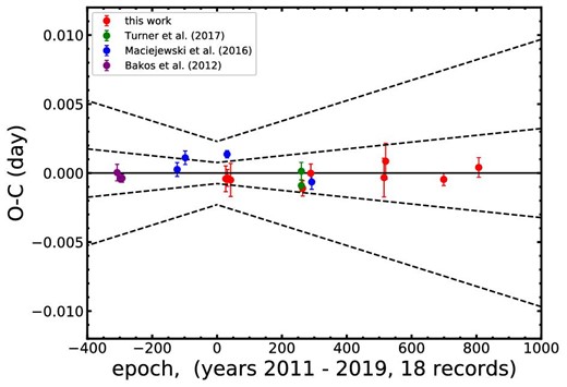
Transit timing variations for HAT-P-37b. The solid line represents zero deviation from the predicted time of transit. The dashed line represents the propagation of ±1σ errors and ±3σ errors associated with the calculated orbital period. The red points represent the mid-transit times obtained from our separate fits with our photometric data, while the blue, green, and pink points represent the mid-transit times cited from Bakos et al. (2012), Maciejewski et al. (2016b), and Turner et al. (2017), respectively. All of the mid-transit times are consistent with our new ephemeris giving an rms scatter of 57 s. (Color online)
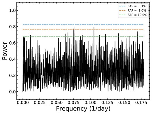
GLS periodogram for all of the data points in the O − C diagram. The FAP-levels (dashed lines) are indicated. (Color online)
4.3 Orbital stability and mass limit of potential perturbers
The mid-transit times derived allow us to constrain the upper mass limit of the potential close-in planetary companions (e.g., Hoyer et al. 2011, 2012; Wang et al. 2019). A perturbing planet can change the linearity of mid-transit times. Nonlinear mid-transit times can induce a large deviation from the ephemeris. As described in Agol et al. (2005), Holman and Murray (2005), and Nesvorný and Morbidelli (2008), based on the rms of scatter around the normal linear ephemeris, TTVs can be used to detect hypothetical close-in planetary companions and constrain their mass.
To calculate the upper mass-limit of potential perturbers, REBOUND (Rein & Liu 2012), an N-body code, was employed to perform the simulation of evolution of this system. For the simulation in this work, the Implicit integrator with Adaptive time Stepping, 15th order (IAS15), was used to perform high-precision long-term orbit integration (Rein & Spiegel 2015).
We assumed that the two planets are coplanar and set in simple circular orbits, which provides the most conservative estimate of the upper limit of the mass of the hypothetical potential perturbers (Bean 2009; Fukui et al. 2011; Hoyer et al. 2011).
In the simulation, we created a grid of periods and masses of hypothetical potential perturbers. To represent the level of stability for each hypothetical potential perturbing planet, the chaos indicator Mean Exponential Growth factor of Nearby Orbits (MEGNO) (Cincotta & Simó 1999, 2000; Cincotta et al. 2003; Hinse et al. 2010) was employed to quantify the degree of the chaos of a nonlinear dynamical system. For the quasi-periodic behavior of the system, the value of MEGNO is close to 2. However, large-scale orbital instabilities can lead to a MEGNO larger than 2. We integrated each pair of initial period and mass for 100000 years and calculated MEGNO at a step of 10 years. To speed up the computation, Parallel Python, a Python package that parallelizes a Python code in a simple way, was employed.4 Therefore, dozens of parallel integrations could be run simultaneously.
For the calculation of the rms scatter of TTVs, we followed a direct brute-force routine. We adopted a gradient descent method (Avriel 2003) to derive every mid-transit time in integration for each grid point. Based on the mid-transit times, the rms scatter of the TTVs of each grid point can be calculated.
The MEGNO map with the perturber mass-limit function is shown in figure 6 with a resolution of 1080 × 786 pixels. The range 0.1 < P2/P1 < 3.5 and 10−2 M⊕ < Mperturber < 10−4 M⊕ was explored to calculate MEGNO and the upper limit of mass of hypothetical perturbers. The location of orbital resonances shows a larger rms scatter of TTVs, where the line corresponding to a TTV signal with an rms of 57 s is shifted downward. For this system, according to our simulations, a perturber with a mass in the range 0.2–200 M⊕ could theoretically lead to a TTVs of 57 s when located in 1 : 3, 1 : 2, 2 : 3 (interior), or 3 : 2, 2 : 1, 5 : 2, 3 : 1 (exterior) orbital resonance. The locations of the resonances have been marked in figure 6.
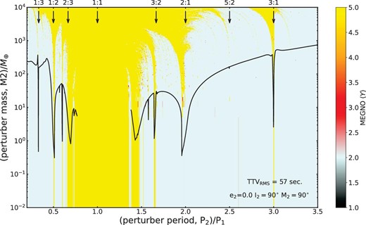
MEGNO map for HAT-P-37. The black solid lines represent the mass of hypothetical perturbing planets than can induce a TTVs of 57 s. Vertical arrows represent the location of (P2/P1) orbital resonances. The behavior of this system is chaotic when the MEGNO value is about 5, marked with yellow area. When the MEGNO value is around 2 (blue region), the system is stable. Vertical arrows indicate the location of (P2/P1) orbital resonances between the transiting planet and a perturber. The mass–period parameter is plotted with a black line, which the perturber introduces a TTV signal with an rms of 57 s as determined by our timing analysis. (Color online)
5 Summary and conclusion
In this work, We observed nine transit light curves of the exoplanetary system HAT-P-37 from 2011 February to 2019 September. We doubled the light curve data compared to the literature.
The nine new transit light curves, along with nine light curves from Bakos et al. (2012), Maciejewski et al. (2016b), and Turner et al. (2017), and RVs from Bakos et al. (2012), were simultaneously modeled. Based on the results of the global fit, we updated the physical and orbital parameters for HAT-P-37, which are in agreement with those from previous works (Bakos et al. 2012; Maciejewski et al. 2016b; Turner et al. 2017). Based on mid-transit times derived from the individual fit for each transit, we present new linear ephemeris (Tc[0] = 2456478.57916 ± 0.00077 [BJDTDB], P = 2.7974415 ± 0.0000025 d).
Moreover, mid-transit times allow us to perform TTVs studies. There is no significant signal in the TTVs of 57 s derived from our transit timing analysis. With precise mid-transit times, we constrain the upper mass limit of hypothetical potential perturbing planets, especially for those planets at the locations of orbital resonance.
To sum up, through the analysis of this work, most of the improved system parameters are more accurate than in previous works. In addition, the ephemeris has been updated to facilitate future follow-up observations. For most of the confirmed exoplanetary systems, this type of follow-up observation is needed to improve the precision of properties of planets and their hosts. These system parameters could influence the formation and evolution of planets. With the discovery of new exoplanets of space telescope missions (e.g., Kepler, TESS, and JWST to be launched) and follow-up observations of ground telescopes, puzzles of exoplanets will be unveiled.
Acknowledgements
Thanks the referee very much for the very valuable and constructive comments to improve this paper a lot. This work is supported by the Joint Research Fund in Astronomy (No. U1931103) under cooperative agreement between National Natural Science Foundation of China (NSFC) and Chinese Academy of Sciences (CAS), and by NSFC (No. 11703016), and by Young Scholars Program of Shandong University, Weihai (No. 20820171006), and by the Chinese Academy of Sciences Interdisciplinary Innovation Team, and by the Open Research Program of Key Laboratory for the Structure and Evolution of Celestial Objects (No. OP201704). This work is partly supported by the Supercomputing Center of Shandong University, Weihai and by China National Astronomical Data Center (NADC), Chinese Virtual Observatory (China-VO), Astronomical Big Data Joint Research Center, co-founded by National Astronomical Observatories, Chinese Academy of Sciences and Alibaba Cloud.
