


Abstract
We investigate gravitational waves with sub-nHz frequencies (10−11 Hz ≲ fGW ≲ 10−9 Hz) from the spatial distribution of the spin-down rates of millisecond pulsars. As we suggested in Yonemaru et al. (2018, MNRAS, 478, 1670), gravitational waves from a single source induce a bias in the observed spin-down rates of pulsars depending on the relative direction between the source and the pulsar. To improve the constraints on the time derivative of gravitational wave amplitude obtained in our previous work (Kumamoto et al. 2019, MNRAS, 489, 3547), we adopt a more sophisticated statistical method called the Mann–Whitney U test. Applying our method to the ATNF pulsar catalogue, we first find that the current data set is consistent with no gravitational wave signal from any direction in the sky. Then, we estimate the effective angular resolution of our method to be 66 deg2 by studying the probability distribution of the test statistic. Finally, we investigate gravitational wave signals from the Galactic Center (GC) and M 87 and, comparing simulated mock data sets with the real pulsar data, we obtain upper bounds on the time derivative as |$\dot{h}_{\rm GC} < 8.9 \times 10^{-19}$| s−1 for the GC and |$\dot{h}_{\rm M87} < 3.3 \times 10^{-19}$| s−1 for M 87, which are stronger than those obtained in Kumamoto et al. (2019, MNRAS, 489, 3547) by factors of 7 and 25, respectively.
1 Introduction
Pulsar timing arrays (PTAs) can detect nHz-frequency gravitational waves (GWs). Although such GWs have not yet been detected, the three major PTA groups, Parkes PTA (Manchester et al. 2013; Kerr et al. 2020), European PTA (Kramer & Champion 2013; Babak et al. 2016), and NANOGrav (Aggarwal et al. 2019; Alam et al. 2021) are operating to detect GWs and have put constraints on the GW amplitudes. These PTA groups also cooperate as the International PTA (Verbiest et al. 2016) in order to improve the sensitivity. In the near future, the Square Kilometre Array (SKA) constructed in Australia and South Africa will appear and discover about 27000 pulsars, including about 3000 millisecond pulsars (MSPs; Keane et al. 2015; Kramer & Stappers 2015), and further improve the sensitivity. Thus, PTAs will greatly promote multi-wavelength gravitational wave astronomy.
Nanohertz-frequency GWs are radiated from supermassive black hole (SMBH) binaries in galactic cores. Their frequency, fGW, is determined by the separation a and reduced mass μ of the binary; typically, fGW ∼ 10−8 Hz for a ∼ 10−2 pc and μ = 2.5 × 10⁸ M⊙. On the other hand, the frequency of GWs observable by PTAs is determined by the observational time span and cadence. The practical range is typically 10−9 ≲ fGW ≲ 10−6 Hz. This frequency range corresponds to the late stage of evolution of the binary.
We need to detect sub-nHz frequency GWs to probe the early phase of binary evolution, in particular to treat the final parsec problem (Milosavljević & Merritt 2003; Ryu et al. 2018). For stochastic GW backgrounds with sub-nHz frequencies, several detection methods have been proposed so far (Bertotti et al. 1983; Kopeikin 1997; Pshirkov 2010). Bertotti, Carr, and Rees (1983) estimated the contribution from stochastic GW backgrounds to the timing noise of pulsars and suggested that they can be distinguished from the intrinsic irregularities of pulsars by searching for correlations between the timing noise of different pulsars. Kopeikin (1997), using binary pulsars, placed a limit on the energy density of GW backgrounds of ΩGWh2 ≲ 2.7 × 10⁻⁴ in the frequency range 1.1 × 10⁻¹¹ Hz < fGW < 4.5 × 10⁻⁹ Hz, where h is the Hubble constant. Pshirkov (2010) suggested a new method for exploring GW backgrounds in the frequency range 10−12–10−8 Hz. This method is based on precise measurements of pulsar periods. The second derivative of the periods from a number of pulsars gave a constraint of ΩGWh2 ≲ 10−6. For similar previous work, see, e.g., Iorio (2014).
Yonemaru et al. (2016) proposed a new method for detecting sub-nHz GWs from a single source with the statistics of spin-down rates of MSPs. This work was motivated by the possible existence of a second SMBH in M 87 indicated by the significant displacement of the active galactic nucleus from the luminous center of M 87 (Batcheldor et al. 2010). As we describe in section 2, sub-nHz GWs induce a bias on the observed spin-down rates of MSPs depending on the relative direction between the GW source and a pulsar. According to the sign of the bias factor, the celestial sphere is divided into two regions: one with a positive bias and the other with a negative bias. Then, GWs can be probed by measuring the statistical difference in the distribution of spin-down rates between two pulsar groups from the positive and negative bias. Yonemaru et al. (2018) gave a rough estimate of the potential sensitivity using a simple model of the distribution of pulsar positions, with skewness as a statistical quantity to characterize the distribution of spin-down rates: the skewness difference between the two groups was considered to be a measure of GW signals. Hisano et al. (2019) adopted a realistic model of the pulsar spatial distribution within the Galaxy to improve the prediction of the sensitivity. Then, Kumamoto et al. (2019) derived upper bounds on the time derivative of the GW amplitudes from two possible GW sources, the Galactic Center (GC) and M 87.
In this study we attempt to improve the constraints given by Kumamoto et al. (2019) by adopting a more sophisticated statistical method, the Mann–Whitney U test. In section 2 we review the basic idea for the detection of sub-nHz frequency GWs from the statistics of the spin-down rates. We describe the details of the pulsar catalogue we employ in this work in section 3, and the Mann–Whitney U test is introduced in section 4. Our main results, constraints on the time derivative of GW amplitudes and the estimation of the effective angular resolution of our method, are presented in section 5. We give discussions and interpretations of the results in section 6, and a summary is provided in section 7.
2 Detection principle
In this work we focus on GWs with a period much longer than the observational time span, which is typically 10 yr. Then the effect of GWs with a much longer period can be approximated as a linear function in the time domain.
The bias factor has a quadrupole spatial pattern centered at the GW source position, and the celestial sphere is divided into two areas which have positive and negative values of the bias factor |$\alpha (\hat{\boldsymbol \Omega },\hat{\boldsymbol p},\theta )$|, as shown in figure 1. Therefore, a statistical difference in the observed spin-down rates is induced between two pulsar groups from the positive and negative regions. In Kumamoto et al. (2019), the skewness of the spin-down rate distribution was considered and the skewness difference between the two regions was used to quantify the statistical difference.
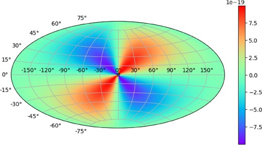
Spatial pattern of the bias factor in the sky for |$\dot{h}_+$| = |$10^{-18}\, {{\textsf {s}}}^{-1}$|. The GW source is placed at the center of the sky in equatorial coordinates and the polarization angle is set to θ = 0°. (Color online)
3 Pulsar catalogue
In this work, we obtain observed MSP data from the Australia Telescope National Facility (ATNF) Pulsar Catalogue (psrcat) version 1.62 (Manchester et al. 2005). It includes 274 MSPs with a measured period shorter than 30 |$\rm {ms}$| and a measured time derivative. We exclude 72 MSPs in globular clusters since they would be biased significantly by the gravitational potential and complicated dynamics inside the cluster. In addition, two MSPs are removed as outliers: one with a negative spin-down rate (|$\dot{P}_{\rm obs}/{P} = -10^{-20.2}\, [{\rm s}^{-1}]$|, J1801−3210) and one with an exceptionally large spin-down rate (|$\dot{P}_{\rm obs}/{P} = 10^{-11.5}\, [{\rm s}^{-1}]$|, J0537−6910). Thus, just 200 MSPs are used for our analysis below. However, it should be noted that our method based on the Mann–Whitney U statistic explained below is rather robust to the presence of outliers and the results should not be affected significantly by the removal.
Figure 2 shows the histogram of logarithmic spin-down rates (|$\dot{P}_{\rm obs}/{P}$|) of the 200 observed MSPs. The mean and standard-deviation of this distribution are −17.46 and 0.47, respectively. The positions of the 200 MSPs in the sky are shown in figure 3 in equatorial coordinates. The positions of the GC and M 87 are also shown.
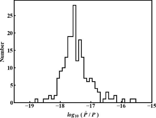
Histogram of logarithmic spin-down rates (|$\dot{P}_{\rm obs}/{P}$|) of the 200 MSPs considered.
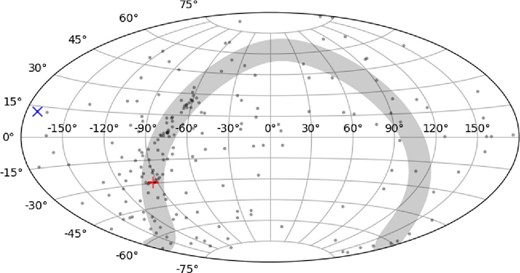
Positions of the 200 MSPs in the sky in equatorial coordinates. The red “+” and blue “×” show the positions of the GC and M 87, respectively. The gray shadowed region represents the Galactic plane. (Color online)
4 Mann–Whitney U test
5 Results
5.1 GW searching
As a demonstration, in figure 4 we show the z test statistic as a function of the polarization angle toward the GC and M 87, |${z}(\hat{\boldsymbol r}_{\rm GC},\theta )$| and |${z}(\hat{\boldsymbol r}_{\rm M87},\theta )$|. As can be seen, it rapidly varies with the polarization angle, and the maximum values are |${z}_{\rm max}(\hat{\boldsymbol r}_{\rm GC}) = 2.55$| and |${z}_{\rm max}(\hat{\boldsymbol r}_{\rm M87}) = 1.43$|, respectively. Figure 5 shows the distribution of |${z}_{\rm max}(\hat{\boldsymbol r})$| in the sky. Here, |${z}_{\rm max}(\hat{\boldsymbol r})$| is depicted for every 5° in RA and Dec, and |${z}(\hat{\boldsymbol r},\theta )$| was calculated for every 10° of the polarization angle to perform the maximization. There are several hot spots where the value of |${z}_{\rm max}(\hat{\boldsymbol r})$| is relatively large (>3), and the largest value is zMAX = 3.8. The directions of this maximum value and its antipode are (105°, −3°), away from both the GC and M 87.
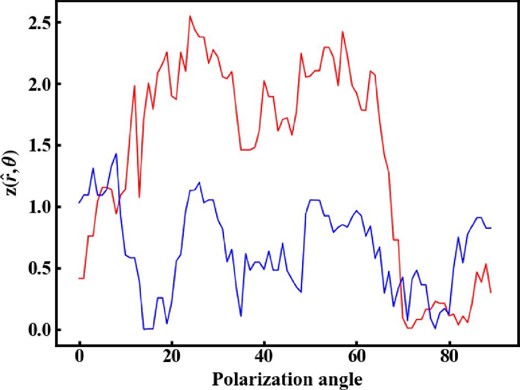
z test statistic as a function of polarization angle toward the GC (red) and M 87 (blue), |${z}(\hat{\boldsymbol r}_{\rm GC},\theta )$| and |${z}(\hat{\boldsymbol r}_{\rm M87},\theta )$|. The maximum values are |${z}_{\rm max}(\hat{\boldsymbol r}_{\rm GC}) = 2.55$| and |${z}_{\rm max}(\hat{\boldsymbol r}_{\rm M87}) = 1.43$|, respectively. (Color online)
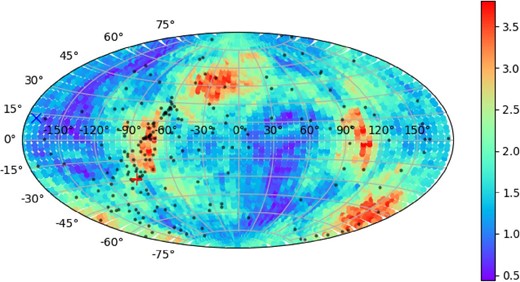
Distribution of |${z}_{\rm max}(\hat{\boldsymbol r})$| in the sky. The black points represent the positions of 200 MSPs. The red “+” and blue “×” show the positions of the GC and M 87, respectively. (Color online)
Here, the value of |${z}_{\rm max}(\hat{\boldsymbol r})$| itself does not directly represent the significance of the GW signal due to the anisotropy of pulsar distribution in the sky. To evaluate the statistical significance, we perform a series of Monte Carlo simulations. In this subsection we first test the significance of the maximum value over the entire sky, zMAX = 3.8, and then we test the significance and put constraints on GWs toward specific directions, GC and M 87, in subsection 5.3.
First, we make a mock data set of spin-down rates (|$\dot{P}_{\rm obs}/{P}$|) for 200 MSPs located at the same positions as those observed. Each MSP is given a value of logarithmic spin-down rate (|$\log {\dot{P}/P}$|) randomly following the Gaussian distribution with the same mean and standard deviation as the real data (−17.46 and 0.47, respectively). Then, we calculate the z test statistics in the same way as above. We perform this simulation 1000 times and obtain the probability distribution of zMAX.
Figure 6 shows the probability distribution of zMAX. The distribution extends from 2.0 to 4.5 and is peaked at around 3. The observed value of zMAX = 3.8, indicated by the vertical line, is slightly larger than the average but is consistent with no GW signal.
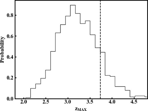
Probability distribution of zMAX obtained from 1000 realizations of a Monte Carlo simulation without GW injection. The vertical dashed line is zMAX = 3.8 obtained from the real data.
5.2 Angular resolution
In this subsection we discuss the effective angular resolution of the GW search in our method. As we saw in figure 5, although we plotted it for every 5°, the spatial pattern of |${z}_{\rm max}(\hat{\boldsymbol r})$| varies at a much larger scale of about 20°. This indicates that the values of |${z}_{\rm max}(\hat{\boldsymbol r})$| for adjacent pixels are not statistically independent. Thus, it is expected that the angular resolution for a GW source will be about the same order as the spatial pattern, if it is detected by our method.
The effective angular resolution can be evaluated by the statistical behavior of the z test statistic. First, we show the probability distribution of |${z}(\hat{\boldsymbol r},\theta )$| in figure 7. This is calculated using the z values of all positions in the sky and the polarization angles of the real data. The distribution is reproduced well by a truncated normal distribution, which is the distribution of an absolute value which follows a normal distribution. The mean and standard-deviation of the normal distribution (not the truncated normal distribution) are 0.0 and 1.08, respectively.
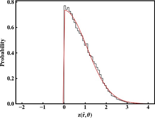
Probability distribution of |${z}(\hat{\boldsymbol r},\theta )$| calculated using the z values of all positions in the sky and polarization angles of the real data. The red curve is the truncated normal distribution. See the main text for the details. (Color online)
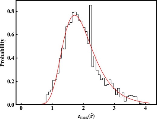
Histogram of |${z}_{\rm max}(\hat{\boldsymbol r})$| shown in figure 5. The red solid line represents the best-fitting Gumbel distribution with a location parameter of 1.72 and a scale parameter of 0.48. (Color online)
5.3 Constraints on the time derivative of GW amplitude
Finally, we derive constraints on the time derivative of the GW amplitude focusing on two specific potential GW source candidates: GC and M 87. As we saw in subsection 5.1, we had the maximized z test statistics toward these directions as |${z}_{\rm max}(\hat{\boldsymbol r}_{\rm GC}) = 2.55$| and |${z}_{\rm max}(\hat{\boldsymbol r}_{\rm M87}) = 1.43$|, respectively.
We evaluate the statistical significance of these values with Monte Carlo simulations similar to those described in subsection 5.1, but here we inject the GW signal in order to derive constraints on the time derivative of GW amplitude. Therefore, to obtain mock observed spin-down rates, |$\dot{P}_{\rm obs}/{P}$|, we need to add the bias factor, |$\alpha (\hat{\boldsymbol \Omega },\hat{\boldsymbol p},\theta )$|, to the mock intrinsic spin-down rates, |$\dot{P}_0/{P}$|, generated randomly from the normal distribution [see equation (12)].
Figure 9 shows the probability distribution of |${z}_{\rm max}(\hat{\boldsymbol r}_{\rm GC})$| and |${z}_{\rm max}(\hat{\boldsymbol r}_{\rm M87})$| obtained from 10000 realizations of simulations with and without the GW signal. As the GW signal get stronger, the probability distribution moves rightward. We regard a value of |$\dot{h}$| as an upper bound, when the probability that |${z}_{\rm max}(\hat{\boldsymbol r})$| is smaller than the observed value, indicated by the vertical line, is 2% with the assumed GW signal. We obtained upper bounds of |$\dot{h}_{\rm GC} < 8.9 \times 10^{-19}\, {\rm s}^{-1}$| for the GC and |$\dot{h}_{\rm M87} < 3.3 \times 10^{-19}\, {\rm s}^{-1}$| for M 87. We discuss the implications of these upper bounds in section 6.
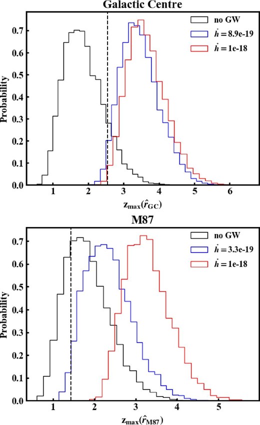
Probability distribution of the maximized z test statistics |${z}_{\rm max}(\hat{\boldsymbol r})$| without the GW signal (black) and with the GW signals (red and blue). The top panel is for the GC and the red and blue lines correspond to values of |$\dot{h}$| of 10−18 s−1 and 8.9 × 10⁻¹⁹ s−1, respectively. The bottom panel is for M 87, and the red and blue lines correspond to values of |$\dot{h}$| of 10−18 s−1 and 3.3 × 10⁻¹⁹ s−1, respectively. The vertical dashed lines are the observed values of |${z}_{\rm max}(\hat{\boldsymbol r})$|. (Color online)
6 Discussions
First, let us compare the results with our previous work. As mentioned in section 1, Kumamoto et al. (2019) placed constraints on the time derivative of the GW amplitude with the skewness difference as the indicator. In consequence, we obtained |$\dot{h}_{\rm GC} < 6.2 \times 10^{-18}\, {\rm s}^{-1}$| for GC and |$\dot{h}_{\rm M87} < 8.1 \times 10^{-18}\, {\rm s}^{-1}$| for M 87. Therefore, the current constraints are stronger by factors of 7 and 25 for GC and M 87, respectively.
In fact, in the current analysis we employed the ATNF pulsar catalogue version 1.62, which includes 50 more MSPs than the catalogue version 1.59 which was employed in Kumamoto et al. (2019). Thus, it is possible that the improvement of the constraints is due to the increased number of MSPs, rather than the change of methodology. To see this, we repeated the current analysis with MSPs from the catalogue version 1.59. As a result, we obtained maximum z statistics of |${z}_{\rm max}(\hat{\boldsymbol r}_{\rm GC}) = 2.27$| and |${z}_{\rm max}(\hat{\boldsymbol r}_{\rm M87}) = 2.02$|, and upper bounds of |$\dot{h}_{\rm GC} < 8.3 \times 10^{-19}\, {\rm s}^{-1}$| for the GC and |$\dot{h}_{\rm M87} < 9.0 \times 10^{-19}\, {\rm s}^{-1}$| for M 87. The constraint for the GC is comparable to the one from the fiducial analysis. On the other hand, constraints for M 87 is degraded by a factor of 3 but is still better than the constraint in Kumamoto et al. (2019) by a factor of 9. Thus, we conclude that the current method with the Mann–Whitney U test is more effective than the previous method with the skewness difference. The comparison of the constraints is summarized in table 1.
Comparison of the constraints on |$\dot{h}$|.
| Kumamoto et al. | U test with | ||
|---|---|---|---|
| GW source | This work | (2019) | catalogue ver. 1.59 |
| GC | 8.9 × 10⁻¹⁹ | 6.2 × 10⁻¹⁸ | 8.3 × 10⁻¹⁹ |
| M 87 | 3.3 × 10⁻¹⁹ | 8.1 × 10⁻¹⁸ | 9.0 × 10⁻¹⁹ |
| Kumamoto et al. | U test with | ||
|---|---|---|---|
| GW source | This work | (2019) | catalogue ver. 1.59 |
| GC | 8.9 × 10⁻¹⁹ | 6.2 × 10⁻¹⁸ | 8.3 × 10⁻¹⁹ |
| M 87 | 3.3 × 10⁻¹⁹ | 8.1 × 10⁻¹⁸ | 9.0 × 10⁻¹⁹ |
In the SKA era, we will have 3000 MSPs (Keane et al. 2015; Kramer & Stappers 2015) and the constraint on ultra-low-frequency GWs considered here will be improved accordingly. In fact, Hisano et al. (2019) estimated the future constraints with the skewness difference and obtained |$\dot{h} < 2 \times 10^{-19}\, {\rm s}^{-1}$| at fGW = 10−11 Hz for the GC, which is stronger than the constraint obtained in Kumamoto et al. (2019) by a factor of 30. It is possible that a future constraint based on the Mann–Whitney U test statistics will be improved by a similar factor, although detailed Monte Carlo simulations to confirm this are beyond the scope of the current paper. This possibility will be pursued elsewhere.
On the other hand, a longer observation time has indirect effects on upper limits. To determine the pulsar period and its derivative precisely, we need observations with a time span of O(1) yr. However, once we have sufficiently precise values on these parameters, an even longer observation time does not improve the upper limit any further.
7 Conclusions
We constrained the time derivative of GW amplitude with sub-nHz frequencies (10−11 Hz ≲ fGW ≲ 10−9 Hz) from the spatial distribution of the spin-down rates of MSPs. As suggested by Yonemaru et al. (2018), GWs from a single source induce a bias in the observed spin-down rates of pulsars depending on the relative direction between the GW source and the pulsar. Compared with our previous studies (Yonemaru et al. 2018; Hisano et al. 2019; Kumamoto et al. 2019), where the skewness difference in the spin-down rate distribution was considered to detect the bias, we adopted a more sophisticated statistical method called the Mann–Whitney U test.
Applying our method to the ATNF Pulsar Catalogue version 1.62, we first found that the maximized value of the z test statistic obtained from the current data set is consistent with no GW signal from any direction in the sky. Then, we estimated the effective angular resolution of our method to be (66 deg)2 by studying the probability distribution of the z test statistic. Finally, comparing simulated mock data sets with the real pulsar data, upper bounds on |$\dot{h}$| were derived as |$\dot{h}_{\rm GC} < 8.9 \times 10^{-19}\, {\rm s}^{-1}$| for the GC and |$\dot{h}_{\rm M87} < 3.3 \times 10^{-19}\, {\rm s}^{-1}$| for M 87, which are stronger than those obtained by Kumamoto et al. (2019) by factors of 7 and 25, respectively. These constraints would be improved significantly with the 3000 MSPs expected to be discovered by the SKA.
Acknowledgements
The Parkes telescope is part of the Australia Telescope National Facility which is funded by the Commonwealth of Australia for operation as a National Facility managed by CSIRO. The ATNF Pulsar Catalogue at 〈https://www.atnf.csiro.au/research/pulsar/psrcat/〉 was used for this work. KT is partially supported by JSPS KAKENHI Grant Numbers JP15H05896, JP16H05999, and JP17H01110, and Bilateral Joint Research Projects of JSPS. SH is supported by JSPS KAKENHI Grant Number JP20J20509.
