Particle–particle particle–tree code for planetary system formation with individual cut-off method: GPLUM

Ishigaki, Yota; Kominami, Junko; Makino, Junichiro; Fujimoto, Masaki; Iwasawa, Masaki

doi:10.1093/pasj/psab028

Abstract

In a standard theory of the formation of the planets in our Solar System, terrestrial planets and cores of gas giants are formed through accretion of kilometer-sized objects (planetesimals) in a protoplanetary disk. Gravitational N-body simulations of a disk system made up of numerous planetesimals are the most direct way to study the accretion process. However, the use of N-body simulations has been limited to idealized models (e.g., perfect accretion) and/or narrow spatial ranges in the radial direction, due to the limited number of simulation runs and particles available. We have developed new N-body simulation code equipped with a particle–particle particle–tree (P³T) scheme for studying the planetary system formation process: GPLUM. For each particle, GPLUM uses the fourth-order Hermite scheme to calculate gravitational interactions with particles within cut-off radii and the Barnes–Hut tree scheme for particles outside the cut-off radii. In existing implementations, P³T schemes use the same cut-off radius for all particles, making a simulation become slower when the mass range of the planetesimal population becomes wider. We have solved this problem by allowing each particle to have an appropriate cut-off radius depending on its mass, its distance from the central star, and the local velocity dispersion of planetesimals. In addition to achieving a significant speed-up, we have also improved the scalability of the code to reach a good strong-scaling performance up to 1024 cores in the case of N = 10⁶.

1 Introduction

In the standard model of planetary system formation, planets are considered to form from planetesimals. While how (and whether) planetesimals form in a protoplanetary disk is still under debate, a standard scenario assumes that a protoplanetary disk was initially filled with numerous planetesimals and the evolution of the system through gravitational interactions among planetesimals is considered to realize the scenario described below.

Planetesimals coagulate and form runaway bodies within about 10⁵ yr (e.g., Kokubo & Ida 1996). This is called the runaway phase, and is followed by the oligarchic phase (e.g., Kokubo & Ida 1998) in which the runaway bodies grow until they reach the isolation mass (e.g., Kokubo & Ida 2002). The isolation mass is the mass at which the runaway bodies consume the planetesimals in their neighborhood. The separation distance between runaway bodies is within 5–10 Hill radii. The isolation mass is ∼M_Mars in the terrestrial planet region. In the gas giant and ice giant regions, the isolation mass reaches several times ∼M_⊕. Once the mass of a runaway body reaches the critical value, which is about 10 times the Earth mass, runaway gas accretion starts to form a giant planet, with the runaway body constituting the core of the planet (Mizuno et al. 1978; Mizuno 1980; Ikoma et al. 1998).

One limitation of this scenario is that it is based on a rather limited set of N-body simulations, with a low mass resolution and a narrow radial range. For example, Kokubo and Ida (2002) used particles with a minimum mass of 10²³ g (corresponding to a ∼100 km-sized planetesimal), and a radial range of 0.5–1.5 au.

These limitations imply that our current understanding of the planetary system formation process is based on “local” physical models, in which we assume that the radial migration of seed planetesimals or protoplanets does not affect the formation process significantly. This assumption of locality is, however, clearly insufficient, especially when we recognize that some exoplanetary systems are clearly shaped by migration effects. Protoplanets and planets can shift their radial positions via at least three main mechanisms: Type I migration, planetesimal-driven migration, and interactions between planets. In order to model the planetesimal-driven migration of protoplanets, a mass resolution much higher than in previous N-body simulations is necessary (Minton & Levison 2014). When a protoplanet with a mass larger than typical planetesimals is formed, neighboring planetesimals are disturbed gravitationally. If the planetesimal population is not constructed with a good enough resolution, as in previous studies, the perturbation becomes random, making systematic radial migration artificially absent. To study the effects of migration, a simulation needs to involve a wide spatial range in the radial direction as well.

Both a high resolution and a large spatial extent are, however, computationally demanding. Almost all previous long-term (covering more than 10⁴ yr) simulations have been performed with high-accuracy direct methods (Kokubo & Ida 1996, 1998), and some with acceleration by GRAPE hardware (e.g., Sugimoto et al. 1990; Makino et al. 1993, 2003). Since the calculation cost of the direct method is O(N²), where N is the number of particles, using more than 10⁶ particles to realize a high resolution or a large spatial extent is impractical even with Japanese K computer or its successor, the Fugaku supercomputer, unless a new calculation scheme is introduced.

Oshino, Funato, and Makino (2011) developed a numerical algorithm which combines the fast Barnes–Hut tree method (Barnes & Hut 1986) and an accurate and efficient individual time step Hermite integrator (Aarseth 1963; Makino 1991) through Hamiltonian splitting. This algorithm is called the particle–particle–particle–tree, or P³T, algorithm.

Iwasawa et al. (2017) reported the implementation and performance of a parallel P³T algorithm developed using the FDPS framework (Iwasawa et al. 2016). FDPS is a general-purpose, high-performance library for particle simulations. Iwasawa et al. (2017) showed that P³T algorithm shows high performance even in simulations with large number of particle (N = 10⁶) and wide radial range (1–11 au). Its performance scales reasonably well for up to 512 cores for one million particles, but with one limitation. The cut-off length used to split the Hamiltonian is fixed and shared by all the particles. Thus, when the mass range of the particles becomes large through the runaway growth, the calculation efficiency is reduced substantially. If we take into account the collisional disruption of planetesimals, this problem becomes even more serious.

In this paper we report on the implementation and performance of the GPLUM code for large-scale N-body simulation of planetary system formation, based on a parallel P³T algorithm with individual mass-dependent cut-off length. We will show that the use of individual mass-dependent cut-off can speed up a calculation by a factor of 3–40.

In section 2 we describe the implementation of GPLUM. Section 3 is devoted to performance evaluation, and section 4 provides discussion and conclusion.

2 Numerical method

If the fourth-order Hermite scheme with individual time step (Aarseth 1963) is used, the order of the calculation cost becomes O(N²), where N is the number of particles. Hence, the cost of calculations increases significantly as N increases. Simulations using parallelized code on ther Japanese K computer (e.g., Kominami et al. 2016) could treat up to several times 10⁵ particles. They used the Ninja algorithm (Nitadori et al. 2006) for parallelization of the Hermite scheme. On the other hand, in order to increase the number of particles that can be treated, the tree method (Barnes & Hut 1986) has been used at the expense of numerical accuracy. In order to improve both accuracy and speed, a scheme which combines the Barnes–Hut tree scheme and the high-order Hermite scheme (P³T) with individual time step has been developed. We incorporate this P³T scheme into our code.

In this section we describe the concept and the implementation of our code, GPLUM.

2.1 Basic equations

2.1.1 The P³T scheme

The P³T scheme (Oshino et al. 2011) is a hybrid integrator based on the splitting of the Hamiltonian. In this scheme, the Hamiltonian of the system of particles is divided into two parts by the distances between particle pairs. They are called the soft part and the hard part. The Hamiltonian used in the P³T scheme is given by

$$\begin{eqnarray} H & = & H_{\rm Soft}+H_{\rm Hard}, \end{eqnarray}$$

(1)

$$\begin{eqnarray} H_{\rm Soft} & = & -\sum _{i}^{}\sum _{j>i}^{}\frac{Gm_{i}m_{j}}{r_{ij}}W(r_{ij};r_{\rm out}), \end{eqnarray}$$

(2)

$$\begin{eqnarray} H_{\rm Hard} &=& \sum _{i}^{}\left( \frac{|\boldsymbol {p}_{i}|^{2}}{2m_{i}}-\frac{GM_{*}m_{i}}{r_{i}} \right)\nonumber \\ && -\sum _{i}^{}\sum _{j>i}^{}\frac{Gm_{i}m_{j}}{r_{ij}}\left[ 1-W(r_{ij};r_{\rm out}) \right], \end{eqnarray}$$

(3)

$$\begin{eqnarray} \boldsymbol {r}_{ij} & = & \boldsymbol {r}_{i}-\boldsymbol {r}_{j}, \end{eqnarray}$$

(4)

where G is the gravitational constant, M_* is the mass of the central star, and m_i, |$\boldsymbol {p}_{i}$|⁠, and |$\boldsymbol {r}_{i}$| are the mass, the momentum, and the position of the ith particle, respectively. We did not include the indirect term. W(r_ij; r_out) is the changeover function for the Hamiltonian. Though the changeover function is determined by both outer and inner cut-off radii (see Oshino et al. 2011), we can express this function by the outer cut-off radius alone. This is because the inner cut-off radius is set as r_in = γr_out, where r_in and r_out are the inner and outer cut-off radii and γ is a constant parameter in the range of 0 to 1.

The forces derived from the Hamiltonian are given by

$$\begin{eqnarray} \boldsymbol {F}_{{\rm Soft},i}&=&-\frac{\partial H_{\rm Soft}}{\partial \boldsymbol {r}_{i}}\nonumber \\ &=&-\sum _{j\not=i}^{}\frac{Gm_{i}m_{j}}{{r_{ij}}^{3}}K(r_{ij};r_{\rm out})\boldsymbol {r}_{ij}, \end{eqnarray}$$

(5)

$$\begin{eqnarray} \boldsymbol {F}_{{\rm Hard},i}&=&-\frac{\partial H_{\rm Hard}}{\partial \boldsymbol {r}_{i}}\nonumber \\ &=&-\frac{GM_{*}m_{i}}{{r_{i}}^{3}}\boldsymbol {r}_{i}\nonumber \\ &&-\sum _{j\not=i}^{}\frac{Gm_{i}m_{j}}{{r_{ij}}^{3}}\left[ 1-K(r_{ij};r_{\rm out}) \right]\boldsymbol {r}_{ij}, \end{eqnarray}$$

(6)

where K(r_ij; r_out) is the changeover function for the force, defined by

$$\begin{eqnarray} W(r)=r\int _{r}^{\infty }\frac{K(\bar{r})}{\bar{r}^{2}}d\bar{r}. \end{eqnarray}$$

(7)

The changeover function K(r_ij; r_out) is determined so that it becomes zero when r_ij < r_in and unity when r_ij > r_out. In GPLUM, we use the same changeover functions as PENTACLE (Iwasawa et al. 2017), which is defined by

$$\begin{eqnarray} W(y;\gamma )=\left\lbrace \begin{array}{ll}\frac{7(\gamma ^6-9\gamma ^5+45\gamma ^4-60\gamma ^3\ln \gamma -45\gamma ^2+9\gamma -1)}{3(\gamma -1)^7}y & (y<\gamma ) , \\ f(y;\gamma )+\left[1-f(1;\gamma )\right]y&(\gamma \le y<1) , \\ 1&(1\le y) , \end{array}\right.\!\!\!\!\nonumber\\ \end{eqnarray}$$

(8)

where

$$\begin{eqnarray} f(y;\gamma )&=&\Bigl \lbrace -10/3y^7 + 14(\gamma +1)y^6 -21(\gamma ^2+3\gamma +1)y^5\nonumber \\ &&+\left[ 35(\gamma ^3+9\gamma ^2+9\gamma +1)/3 \right]y^4-70(\gamma ^3+3\gamma ^2\nonumber \\ &&+\gamma )y^3+210(\gamma ^3+\gamma ^2)y^2-140\gamma ^3y\ln y\nonumber \\ &&+(\gamma ^7-7\gamma ^6+21\gamma ^5-35\gamma ^4)\Bigr \rbrace/ (\gamma -1)^7. \end{eqnarray}$$

(9)

Since the changeover function becomes unity when r_ij > r_out, gravitational interactions of the hard part work only between particles within the outer cut-off radius. We call particles within the outer cut-off radius “neighbors.” Hence, to integrate the hard part, it is sufficient to consider clusters composed of neighboring particles, which we call “neighbor clusters.” We will explain the procedure of time integration and the definition of neighbors and neighbor clusters in subsection 2.2.

The Hamiltonian equation of motion is written as

$$\begin{eqnarray} \frac{{d}w}{{d}t}=\left\lbrace w,H\right\rbrace , \end{eqnarray}$$

(10)

where w is the canonical variable in the phase space and {, } denotes Poisson bracket. The general solution of equation (10) at time t + Δt from t is written as

$$\begin{eqnarray} w(t+\Delta t)=e^{\Delta t \left\lbrace ,H \right\rbrace }w(t) . \end{eqnarray}$$

(11)

In the P³T scheme, the general solution is approximated as

$$\begin{eqnarray} w(t+\Delta t)=e^{\Delta t/2 \left\lbrace ,H_{\rm Soft} \right\rbrace }e^{\Delta t \left\lbrace ,H_{\rm Hard} \right\rbrace }e^{\Delta t/2 \left\lbrace ,H_{\rm Soft} \right\rbrace }w(t). \end{eqnarray}$$

(12)

The P³T scheme adopts the concept of the leapfrog scheme. An image of the procedures of the P³T scheme is shown in figure 1. In the leapfrog scheme, the Hamiltonian is split into free motion and gravitational interactions. In the mixed variable symplectic (MVS) scheme, it is split into Kepler motion and interactions between particles. In the P³T scheme, it is split into the hard part and the soft part. The hard part consists of motion due to the central star and short-range interactions. The soft part consists of long-range interactions. Calculation of the gravitational interactions of the soft part is performed using the Barnes–Hut tree scheme (Barnes & Hut 1986) available in FDPS (Iwasawa et al. 2016). Time integration of the hard part is performed using the fourth-order Hermite scheme (Makino 1991) with the individual time step scheme (Aarseth 1963) for each neighbor cluster, or by solving the Kepler equation with Newton–Raphson iteration for particles without neighbors.

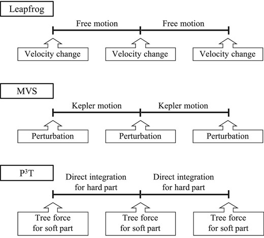
Procedures of the leapfrog (top), MVS (middle), and P3T schemes (bottom). Modified from figure 1 in Fujii et al. (2007).

Fig. 1.

Procedures of the leapfrog (top), MVS (middle), and P³T schemes (bottom). Modified from figure 1 in Fujii et al. (2007).

Open in new tab Download slide

Here we explain how we determine the (outer) cut-off radius r_out. First, we explain the method used to determine the cut-off radius in previous P³T implementations such as PENTACLE. Our new method is explained in sub-subsections 2.1.2 and 2.1.3.

The cut-off radius is determined based on the Hill radius of each particle, which is defined as r_{Hill, i} = [m_i/(3M_*)]^1/3a_i. Here, a_i is the orbital semi-major axis of the particle. The cut-off radius of the ith particle is given by

$$\begin{eqnarray} r_{{\rm out},i} = \tilde{R}_{{\rm cut},0}r_{{\rm Hill},i}, \end{eqnarray}$$

(13)

where |$\tilde{R}_{{\rm cut},0}$| is a parameter. If we use a fixed value for all gravitational interactions as the cut-off radius, the cut-off radius used in equations (2), (3), (5), and (6) can be written as

$$\begin{eqnarray} r_{\rm out} = \max _{k}\left( r_{{\rm out},k} \right). \end{eqnarray}$$

(14)

We call the use of equation (14) the “shared cut-off” method.

2.1.2 The P³T scheme with individual cut-off

Particles can have different cut-off radii. In our new scheme, these different values are actually used for different particles.

The cut-off radius for gravitational interactions between the ith and jth particles is given by

$$\begin{eqnarray} r_{{\rm out},ij} = \max \left( r_{{\rm out},i}, r_{{\rm out},j}\right). \end{eqnarray}$$

(15)

We call the use of equation (15) the “individual cut-off” method.

The parameter |$\tilde{R}_{{\rm cut},0}$| should satisfy |$\tilde{R}_{\rm cut} \ge 1$| if we have to ensure that gravitational interactions with particles closer than the distance of the Hill radius are included in the hard part, or |$\gamma \tilde{R}_{\rm cut} \ge 1$| if we have to ensure that the whole of the gravitational force exerted by particles closer than the Hill radius is calculated in the hard part. Using the individual cut-off method, we have made it possible to split gravitational interactions efficiently, and to make |$\tilde{R}_{{\rm cut},0}$| relatively large (⁠|$\tilde{R}_{{\rm cut},0}\gtrsim 1$|⁠) without reducing the simulation speed. This method requires some complex procedures when two particles with different cut-off radii collide and merge. We will explain the detail of this procedure in subsection 2.4.

2.1.3 The P³T scheme with Hill radius and random velocity dependent cut-off

The cut-off radius should be chosen so that it is sufficiently larger than v_ranΔt, where v_ran is the random velocity of particles and Δt is the time step for the soft part. The time step should be sufficiently shorter than the time for the particles to move a distance equivalent to their cut-off radii.

In GPLUM, instead of equation (13), the cut-off radius for each particle is set to be

$$\begin{eqnarray} r_{{\rm out},i} = \max \left(\tilde{R}_{{\rm cut},0}r_{{\rm Hill},i}, \tilde{R}_{{\rm cut},1}v_{{\rm ran},i}\Delta t\right) , \end{eqnarray}$$

(16)

where |$\tilde{R}_{{\rm cut},0}$| and |$\tilde{R}_{{\rm cut},1}$| are the parameters, and v_{ran, i} is the mean random velocity for particles around the ith particle, where “random velocity” means the difference between the velocity of the particle and the Kepler velocity. Here we call the method of equation (16) the “Hill radius and random velocity dependent cut-off” method.

The parameter R_{cut, 1} should be determined so that it satisfies R_{cut, 1} ≥ 1 in order to let the cut-off radius be sufficiently larger than the product of the random velocity and the time step. We usually use R_{cut, 1} = 8.

To summarize, in GPLUM, when we use both individual cut-off and Hill radius and random velocity dependent cut-off methods, the cut-off radius for gravitational interactions between the ith and jth particles is given by

$$\begin{eqnarray} r_{{\rm out},ij} = \max &&\Bigl (\tilde{R}_{{\rm cut},0}r_{{\rm Hill},i}, \tilde{R}_{{\rm cut},1}v_{{\rm ran},i}\Delta t,\nonumber \\ &&\,\,\,\,\tilde{R}_{{\rm cut},0}r_{{\rm Hill},j}, \tilde{R}_{{\rm cut},1}v_{{\rm ran},j}\Delta t \Bigr ). \end{eqnarray}$$

(17)

2.2 Data structure and time-integration procedure

In GPLUM, the data structure for particles, which we call for the soft part, is created using a function in FDPS. The simulation domain is divided into subdomains, each of which is assigned to one MPI process. Each MPI process stores the data of the particles which belong to its subdomain. We call this system of particles the soft system. A particle in the soft system is expressed in a C++ class, which contains as data the index number, mass, position, velocity, acceleration, jerk, time, time step for the hard part, and the number of neighbors. The acceleration of each particle is split into the soft and hard parts using equations (5) and (6) respectively. The jerk of each particle is calculated only for the acceleration of the hard part since jerk is not used in the soft part. Neighbors of the ith particle are defined as particles which exert hard-part force on the ith particle. The definition of neighbors and the process of creating a neighbor list are explained in subsection 2.3.

For each time step of the soft part, another set of particles is created for the time integration of the hard part. We call this secondary set of particles the hard system. The data of the particles are copied from the soft system to the hard system. A particle in the hard system has second- and third-order time derivatives of the acceleration and the neighbor list, in addition to the data copied from the soft system. These “hard particles” are split into smaller particle clusters, called “neighbor clusters.” Neighbor clusters are created so that, for any member of one cluster, all its neighbors are also members of that cluster. The definition of neighbor clusters and the process of creating neighbor clusters are explained in subsection 2.3. Time integration of the hard part can be performed for each neighbor cluster independently since each hard particle interacts only with particles in its neighbor cluster.

The simulation in GPLUM proceeds as follows (see figure 1):

The soft system is created. The index, mass, position, and velocity of each particle are set from the initial conditions.
Data of the soft system is sent to FDPS. FDPS calculates the gravitational interactions of the soft part, and returns the acceleration of the soft part, a_Soft. The neighbor list of each particle is created.
The first velocity kick for the soft part is given, which means that a_SoftΔt/2 is added to the velocity of each particle, where Δt is the time step of the soft part.
The neighbor clusters are created. If there are neighbor clusters of particles stored in multiple MPI processes, the data for particles contained by it are sent to one MPI process (see subsection 2.3). The data of particles are copied from the soft system to the hard system.
The time integration of the hard system is performed using OpenMP and MPI parallelization.
- The time integration of each neighbor cluster is performed using the fourth-order Hermite scheme. If a particle collision takes place, the procedure for the collision is carried out (see subsection 2.4).
- The time integration of each particle without neighbors is performed by solving the Kepler equation.
The data of particles are copied from the hard system to the soft system. If there are newly born fragments, they are added to the soft system.
The data of the soft system is sent to FDPS. FDPS returns the acceleration of the soft part, a_Soft, in the same way as in step 2. The neighbor list for each particle is created again.
The second velocity kick for the soft part is given in the same way as in step 3.
If collisions of particles take place in this time step, the colliding particles are merged and the cut-off radius and the acceleration of the soft part of all particles are recalculated.
Go back to step 3.

2.3 Neighbor cluster creation procedure

A neighbor list is a list of the indices defined for each particle so that the ith particle’s neighbor list contains the particle indices of the ith particle’s neighbors. Here, the ith particle’s neighbors are defined as the particles which are within the cut-off radius the ith particle during the time step of the soft part. Numerically, the ith particle’s neighbors are defined as the particles within the “search radius.”

Here we explain how we create the neighbor list of each particle in GPLUM. First, particles which are candidates for neighbors are listed for each particle by determining the search radius using an FDPS function,

$$\begin{eqnarray} r_{{\rm search},i} = \tilde{R}_{\rm search,0} r_{{\rm out},i} +\tilde{R}_{\rm search,1}v_{{\rm ran},i}\Delta t, \end{eqnarray}$$

(18)

where |$\tilde{R}_{\rm search,0}$| and |$\tilde{R}_{\rm search,1}$| are parameters. |$\tilde{R}_{\rm search,0}$| is set to unity or a value somewhat larger than unity. The second term of equation (18) is added to the search radius in order to include particles which might come into the region within the cut-off radius during the soft step. In GPLUM, in the case of the individual cut-off method, the search radius is also determined individually for each particle as well as the cut-off radius. The search radius concerning the interaction between ith and jth particles is set to the maximum of the search radii of all particles in the case of the shared cut-off method, or the larger of the search radii of the ith and jth particles in the case of the individual cut-off method.

Second, particles in the ith particle’s neighbor list which do not satisfy the following condition are excluded from the neighbor list:

$$\begin{eqnarray} \tilde{R}_{\rm search,2}{r_{{\rm out},ij}} < \left| \boldsymbol {r}_{ij}+\boldsymbol {v}_{ij}\Delta t_{\rm min} \right|, \end{eqnarray}$$

(19)

where |$\boldsymbol {r}_{ij}$| and |$\boldsymbol {v}_{ij}$| are the position and velocity of the ith particle relative to the jth particle, and Δt_min is chosen so that |$\left| \boldsymbol {r}_{ij}+\boldsymbol {v}_{ij}\Delta t_{\rm min} \right|$| takes a maximum (0 < Δt_min < Δt). It can be calculated as:

$$\begin{eqnarray} t_{\rm min}=\left\lbrace \begin{array}{ll}0 & (-\boldsymbol {r}_{ij}\cdot \boldsymbol {v}_{ij}/{{v}_{ij}}^2<0) , \\ -\boldsymbol {r}_{ij}\cdot \boldsymbol {v}_{ij}/{v_{ij}}^2 & (0\le -\boldsymbol {r}_{ij}\cdot \boldsymbol {v}_{ij}/{v_{ij}}^2<\Delta t) , \\ \Delta t & (\Delta t\le -\boldsymbol {r}_{ij}\cdot \boldsymbol {v}_{ij}/{v_{ij}}^2) . \end{array} \right. \end{eqnarray}$$

(20)

This condition means that if the minimum distance between the ith and jth particles is sufficiently greater than the cut-off radius, we exclude them from their neighbor lists. Because the minimum distance can be smaller than the cut-off radius if the relative acceleration is comparable to or greater than the relative velocity, the jth particles in the ith particle’s neighbor list which satisfy |$v_{ij} < \tilde{R}_{\rm search,3}a_{ij}\Delta t/2$| are not excluded from the neighbor list even if they satisfy the condition in equation (19), where a_ij is the acceleration of the ith particle relative to the jth particle and |$\tilde{R}_{\rm search,3}$| is a parameter larger than unity.

After the neighbor lists of all particles are created, the particles are divided into neighbor clusters so that for all particles in a cluster, all of its neighbors are in the same cluster.

In order to determine a neighbor cluster, a “cluster index” is set for each particle using the following steps:

Initially, the cluster index of each particle is set to be the index of the particle (i.e., i for the ith particle).
The cluster index of a particle is set to the minimum of the cluster indices of all its neighbors and itself.
Step ii is repeated until the cluster index of all neighbors and itself become equal.

Particles with the same cluster index belong to the same neighbor cluster.

If there are neighbor clusters with members from more than one MPI process (such as the clusters of blue, cyan, light green, and purple particles in figure 2), the data for particles which belong to such clusters have to be sent to one MPI process so that they can be integrated without the need for communication between MPI processes. Here we explain the procedure to determine the MPI process to which the particle data is sent for each neighbor cluster with members from more than one MPI process. Some particles have neighbors from an MPI process different from their own. Here we call neighbors stored in a different MPI process “exo-neighbors.” The set of rank numbers of MPI processes of neighbors including itself for the ith particle is R_i. For each particle with exo-neighbors, the procedure to construct the neighbor cluster is as follows:

For each particle with exo-neighbors, the cluster index and R_i are exchanged with exo-neighbors of that particle. Then, the cluster index number is set to be the minimum value of the cluster index numbers of all its exo-neighbors and itself, and R_i is updated to the union of R_j of all its exo-neighbors and its R_i.
Fig. 2.
Illustration of particle system and neighbor cluster. The dots represent particles and the lines connecting particles represent that the connected particles are neighbor pairs. Particles of the same color belong to the same neighbor cluster (except for the gray particles), and gray particles are isolated particles. Each divided area represents the area allocated to each MPI process for FDPS (left) and for time integration of the hard part (right). (Color online)
Open in new tab Download slide
Step A is repeated until the cluster index of all exo-neighbors and itself become equal, and the R_j of all its exo-neighbors and its R_i become equal.

After this procedure, for each neighbor cluster, the time integration will be done on the MPI process which has the minimum rank in R_i. Thus, particle data are sent to that MPI process.

Figures 2 and 3 illustrate these procedures. In the state shown in the left panel of figure 2, the neighbor clusters of blue, cyan, light green, and purple particles span over multiple MPI processes. In order to integrate the hard part of each neighbor cluster in one MPI process, the allocation of neighbor clusters to each MPI process should be like the right panel of figure 2. Consider the neighbor cluster of particles a to g in figure 2. Here we assume that a < b < c < d < e < f < g and i < j < k < l. In this case, after repeating step A three times, particles a to g all have a as their cluster index number and {i, j, k, l} as R_i. Therefore, data for particles c to g are sent to MPI process i, and MPI process i receives data from the rank j to k MPI processes.

Fig. 3.

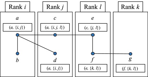
Illustration of neighbor clusters of particles a to g in figure 2 before step A. Here, a to g are the index numbers of each particle, assuming that a < b < c < d < e < f < g. The value in the square under the index number indicates (cluster index number, R_i) the number the particle has before step A. (Color online)

Open in new tab Download slide

Note that our procedure described above is designed to produce no single bottleneck and achieve reasonable load balancing between processes. The communication to construct the neighbor clusters is limited to point-to-point communications between neighboring processes (no global communication), and the time integration is also distributed to many MPI processes.

2.4 Treatment of collisions

2.4.1 Perfect accretion model

Here we explain the procedure for handling collisions for the case of the perfect accretion model.

The procedure for handling collisions is performed during the time integration of the hard part (step 5a, see subsection 2.2). Two particles, which we call the ith and jth particles, are considered to have collided when

$$\begin{eqnarray} r_{ij} < f (R_{{\rm p},i}+R_{{\rm p},j}), \end{eqnarray}$$

(21)

where R_{p, i} and R_{p, j} are the radii of the ith and jth particles respectively. The coefficient f is the enhancement factor of radius. If perfect accretion is assumed, these two particles are replaced by a new particle with mass m_i + m_j, where m_i and m_j are the respective masses of the ith and jth particles. The position and velocity of the new particle are set so that the position of the center of gravity and momentum are conserved:

$$\begin{eqnarray} \boldsymbol {r}_{\rm new} &=& \frac{m_i \boldsymbol {r}_{i}+m_j \boldsymbol {r}_{j}}{m_i+m_j}, \end{eqnarray}$$

(22)

$$\begin{eqnarray} \boldsymbol {v}_{\rm new} &=& \frac{m_i \boldsymbol {v}_{i}+m_j \boldsymbol {v}_{j}}{m_i+m_j}. \end{eqnarray}$$

(23)

The energy dissipation due to the collision is calculated as the summation of the dissipation of the relative kinetic energy and gravitational interaction of two particles, and the change in the interaction energy with others due to the change in position. Thus we have

$$\begin{eqnarray} E_{\rm disp, Hard}&=& \varepsilon _0+\varepsilon _1+\varepsilon _2+\varepsilon _3, \end{eqnarray}$$

(24)

$$\begin{eqnarray} \varepsilon _0&=& \frac{1}{2}\mu _{ij}|\boldsymbol {v}_{ij}|^2, \end{eqnarray}$$

(25)

$$\begin{eqnarray} \varepsilon _1&=&- \frac{Gm_im_j}{r_{ij}}W(r_{ij};r_{{\rm out},ij}), \end{eqnarray}$$

(26)

$$\begin{eqnarray} \varepsilon _2&=&- {GM_*}\left[\frac{m_i}{r_{i}}+\frac{m_j}{r_{j}}-\frac{m_i+m_j}{r_{\rm new}}\right], \end{eqnarray}$$

(27)

$$\begin{eqnarray} \varepsilon _3&=&-Gm_i\sum _{k\in N_i}m_k\left[\frac{W(r_{ik};r_{{\rm out},ik})}{r_{ik}}-\frac{W(r_{{\rm new}k};r_{{\rm out},ik})}{r_{{\rm new}k}}\right]\nonumber \\ &&\!\!- \ Gm_j\sum _{k\in N_j}m_k\left[\frac{W(r_{jk};r_{{\rm out},jk})}{r_{jk}}-\frac{W(r_{{\rm new}k};r_{{\rm out},jk})}{r_{{\rm new}k}}\!\right], \end{eqnarray}$$

(28)

where μ_ij = m_im_j/(m_i + m_j) is the reduced mass and N_i is the neighbor list of the ith particle, ϵ₀ represents the dissipation of the relative kinetic energy of two particles, ϵ₁ the dissipation of gravitational potential between two particles, ϵ₂ the change of gravitational potential with respect to the central star, and ϵ₃ the change of gravitational potential between the neighbors of the ith and jth particles. If the changeover functions in equations (25) to (28) are replaced by unity, the sum of ϵ₀ to ϵ₃ becomes the energy dissipation of the total of the soft and hard parts. Although the gravitational potentials of particles other than neighbors also change, they are ignored. The accuracy of the simulation can be checked by the error in the total energy, taking into account the dissipations mentioned above.

In the case of individual cut-off, the ith and jth particles usually have different cut-off radii. Therefore, the masses m_i and m_j in the new particle are subjected to different hard part forces calculated by the different cut-off radii of the ith and jth particles. However, the masses m_i and m_j should move together as one particle because they have merged. In GPLUM, the new particle (consisting of the ith and jth particles) is considered as composed of two particles. In other words, the ith and jth particles are not replaced by a new particle during the time integration of the hard part. The force on the new particle is calculated in the following steps. First, the hard part accelerations of the ith and jth particles, |$\boldsymbol {a}_ {{\rm Hard},i}$| and |$\boldsymbol {a}_{{\rm Hard},j}$|⁠, are calculated separately, except for the contribution of the interaction between these two particles; then, the hard part acceleration of the new particle is calculated by

$$\begin{eqnarray} \boldsymbol {a}_{{\rm Hard}} &=& \frac{m_i\boldsymbol {a}_{{\rm Hard},i}+m_j\boldsymbol {a}_{{\rm Hard},j}}{m_i+m_j}. \end{eqnarray}$$

(29)

These two particles are replaced by a new particle after the second velocity kick of the soft step (step 9 in subsection 2.2); since the ith and jth particles have different cut-off radii, they feel different soft forces. The acceleration for the soft velocity kick is their mass-weighted average. Thus, there is a small energy dissipation due to this averaging process, expressed as

$$\begin{eqnarray} E_{\rm disp, Soft} = \frac{1}{2}\mu _{ij}|\boldsymbol {v}_{ij}|^2, \end{eqnarray}$$

(30)

where |$\boldsymbol {v}_{ij}$| is the relative velocity of the ith and jth particles right after the velocity kick is given. In the soft part, potential energy dissipation is not present since the particle position does not change before and after merging. After the two particles are merged, the cut-off radius is recalculated. The soft and hard part acceleration and jerk of all particles are recalculated since the change of cut-off radius influences both hard and soft parts of the Hamiltonian.

2.4.2 Implementation of fragmentation

First, we describe how the fragmentation process is treated in the code. The procedure for particle collision with fragmentation is similar to the case of the perfect accretion. When a collision occurs, remnant and fragment particles are created. The number and masses of the remnant and fragments are determined using the fragmentation model.

In GPLUM, as in the case of perfect accretion, mass originating from the ith and jth particles is considered as separate particles until the end of the hard integration steps. We assume that the total mass of the fragments is smaller than the mass of the smaller of the two collision participants. Therefore, we assume that fragments adopt the cut-off radius of the smaller collision participants, and the remnant will be composed of the larger participant and the rest of the mass of the smaller participant.

2.4.3 Fragmentation models

In this section we describe the fragmentation models implemented in GPLUM. Currently, two models are available. One is a very simplified model, which has the advantage that we can study the effect of changing the collision product. The other is a model that can adjust the number of fragments by collision angle and relative velocity based on Chambers (2013), which determines the collision outcome using the result of smooth-particle hydrodynamic collision experimentation. In this model, the collision scenario, which includes accretion, fragmentation, and hit-and-run, is also determied by collision angle and relative velocity. Since the latter is given in Chambers (2013), in the following we describe the simple model only.

We first present the simple model. Here, the mass of the remnant is given by (1 − a)m_i + m_j, where a is a parameter in the range of 0 to 1, and m_i and m_j are the masses of two colliding particles (m_i ≤ m_j). The mass am_i goes to the fragments. The number of fragments, n_frag, is given by

$$\begin{eqnarray} n_{\rm frag} &=& \min \left( \left\lfloor \frac{am_{i}}{m_{\rm min}} \right\rfloor , N_{\rm frag}\right). \end{eqnarray}$$

(31)

Here, m_min is the minimum mass of the particles and N_frag is the maximum number of fragments for one collision. If n_frag = 1, we set it to 0 and apply the procedure for perfect accretion. The fragments all have the same mass,

$$\begin{eqnarray} m_{\rm frag} &=& \frac{am_{i}}{n_{\rm frag}}. \end{eqnarray}$$

(32)

The fragments are placed on a circle with center at the position of the remnant on the plane of the orbital angular momentum of the relative motion of the two particles. The velocities of the fragments relative to the remnant are set to be 1.05 times the escape velocity of the remnant.

The energy dissipation in the hard part due to the collision can be calculated in the same manner as for perfect accretion.

3 Result

3.1 Initial conditions and simulation parameters

In this section we present the initial models, parameters, and computing resources and parallelization method used.

For standard runs we use 10⁶ planetesimals with equal masses of 2 × 10²¹ g distributed in the region 0.9–1.1 au from the Sun. Therefore, the total mass of solid materials is 2 × 10²⁷ g. When we change the total number of particles, the surface mass density is kept unchanged. The solid mass is consistent with that of the minimum-mass Solar nebula (MMSN; Hayashi 1981). Initial orbital eccentricities and inclinations of planetesimals are given by Gaussian distribution with dispersion 〈e²〉^1/2 = 2〈i²〉^1/2 = 2h (Ida & Makino 1992), where h is the reduced Hill radius defined by h = r_Hill/a. The Hill radius r_Hill is given by

$$\begin{equation} r_{\rm Hill} = \left( \frac{m_{\rm p}}{3\, M_\odot }\right)^{1/3}a. \end{equation}$$

(33)

The particle density is set to be 2 g cm⁻³. In the wide-range simulations we use 10⁶ planetesimals with equal masses of 1.5 × 10²⁴ g distributed in the region 1.0–10 au from the Sun.

We use η = 0.01 for the accuracy parameter for the fourth-order Hermite scheme. For the initial step, and also for the first step after a collision, we use η₀ = 0.1η. We set |$\tilde{R}_{\rm search0}=1.1$|⁠, |$\tilde{R}_{\rm search1}=6$|⁠, |$\tilde{R}_{\rm search2}=2$|⁠, and |$\tilde{R}_{\rm search3}=2$| [see equations (17)]. For the accuracy parameter of the Barnes–Hut algorithm we use the opening angle of θ = 0.1 and 0.5. The system of units is that solar mass, the astronomical unit, and the gravitational constant are all unity. In these units, 1 yr corresponds to 2π time units.

The calculations in this paper were carried out on a Cray XC50 system at the Center for Computational Astrophysics (CfCA) of the National Astronomical Observatory of Japan (NAOJ). This system consists of 1005 computer nodes, and each node has Intel Xeon Skylake 6148 (40 cores, 2.4 GHz) processors. We used MPI over up to 208 processors. Unless otherwize noted, OpenMP over five threads and the AVX512 instruction set were used. Some of the calculations were done on on a Cray XC40 system at the Academic Center for Computing and Media Studies (ACCMS) of Kyoto University. This system consists of 1800 computer nodes, and each node has Intel Xeon Phi KNL (68 cores, 1.4 GHz) processors. We used MPI over 272 processes, OpenMP of four threads per process, and the AVX2 instruction set in this system.

We used FDPS version 5.0d (Iwasawa et al. 2016) with the performance enhancement for the exchange of the local essential tree (Iwasawa et al. 2019).

3.2 Accuracy and performance

In sub-subsection 3.2.1 we present the measured accuracy and performance for the case of equal-mass particles, and in sub-subsection 3.2.2 that for systems with a mass spectrum. Finally, in sub-subsection 3.2.3 we present the result of long-term calculations.

3.2.1 Equal-mass systems

In this sub-subsection we present the results of calculations with equal-mass initial models. We use the enhancement factor for particle radius of f = 1. Figure 4 shows the maximum energy error over 10 Keplerian orbits as a function of Δt and |$\Delta t/\tilde{R}_{\rm cut,0}$|⁠. The energy error here is the relative error of the total energy of the system, with corrections for dissipations due to accretion and gas drag when it is included. We have changed the opening angle θ and the cutoff radius |$\tilde{R}_{\rm cut,0}$|⁠. We used individual cut-off in the standard simulation in this section. In narrow-range simulations, the individual cut-off radii are almost the same as the shared cut-off radius since the particle masses are equal.

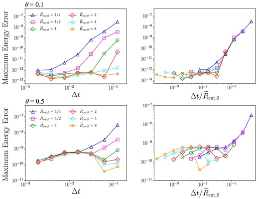
$Maximum energy error over 10 Keplerian orbits as functions of Δt (left) and $\Delta t/\tilde{R}_{\rm cut}$ (right) in the case of θ = 0.1 (top) and θ = 0.5 (bottom). (Color online)$

Fig. 4.

Maximum energy error over 10 Keplerian orbits as functions of Δt (left) and |$\Delta t/\tilde{R}_{\rm cut}$| (right) in the case of θ = 0.1 (top) and θ = 0.5 (bottom). (Color online)

Open in new tab Download slide

For the case of θ = 0.1, the energy error is determined by |$\Delta t/\tilde{R}_{\rm cut,0}$|⁠, and not by the actual value of Δt, as in Iwasawa et al. (2017). The rms value of the random velocity is 2h. Therefore, Δt must be smaller than |$\tilde{R}_{\rm cut,0}$| in order to resolve the changeover function, and that is the reason why the error is determined by |$\Delta t/\tilde{R}_{\rm cut,0}$|⁠. With |$\Delta t/\tilde{R}_{\rm cut,0}< 0.03$|⁠, the integration error reaches the round-off limit of 10⁻¹².

In the case of a larger opening angle, θ = 0.5, the limiting error is around 10⁻¹⁰. This is simply because the acceleration error of the soft part is larger than that for θ = 0.1. Since the cut-off radius and the change of distance due to the relative motion between particles in one step are approximately proportional to |$\tilde{R}_{\rm cut,0}$| and Δt, respectively, it is considered that the energy error is determined by |$\Delta t/\tilde{R}_{\rm cut,0}$|⁠. The reason why the energy error becomes small as |$\tilde{R}_{\rm cut,0}$| and Δt are large when |$\Delta t/\tilde{R}_{\rm cut,0}$| is small could be because the cut-off radius becomes large with |$\tilde{R}_{\rm cut,0}$| and Δt.

Figure 5 shows the maximum energy error over 10 Keplerian orbits as a function of Δt and |$\Delta t/\tilde{R}_{\rm cut,0}$| in a wide-range simulation. The Keperian orbit in this simulation means that of the inner edge. Only the points where the calculation was completed within 30 min are plotted. It shows that the energy error in the case of individual cut-off in a wide-range simulation is not too different from the case of shared cut-off if we use |$\Delta t/\tilde{R}_{\rm cut,0}\lesssim 0.1$|⁠.

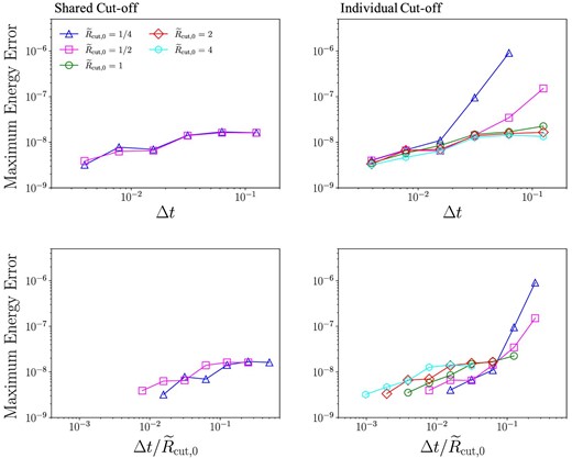
$Maximum energy error over 10 Keplerian orbits as functions of Δt (left) and $\Delta t/\tilde{R}_{\rm cut}$ (right) in the case of θ = 0.5, shared cut-off (left), and individual cut-off (right) in a wide-range simulation. (Color online)$

Fig. 5.

Maximum energy error over 10 Keplerian orbits as functions of Δt (left) and |$\Delta t/\tilde{R}_{\rm cut}$| (right) in the case of θ = 0.5, shared cut-off (left), and individual cut-off (right) in a wide-range simulation. (Color online)

Open in new tab Download slide

Figure 6 shows the wallclock time for the integration over one Kepler time and its breakdown as a function of the number of CPU cores for the case of θ = 0.5, Δt = 1/64, and |$\tilde{R}_{\rm cut,0}=2$|⁠. We used five cores per MPI process. The wallclock time is the average over ten Kepler times. We can see that the parallel performance speed-up is reasonable for up to 320 cores (N = 1.25 × 10⁵) and more than 1040 cores (N = 10⁶).

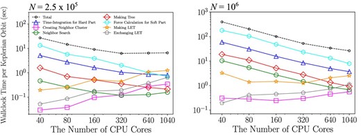
$Wallclock time taken for each procedure per Keplerian orbit as a function of the number of CPU cores in the cases of 1.25 × 105 (left) and 106 (right) particles. We used θ = 0.5, Δt = 1/64, and $\tilde{R}_{\rm cut}=2$. We used five-thread parallelization (i.e., the number of MPI processes is 1/5 of the number of CPU cores). (Color online)$

Fig. 6.

Wallclock time taken for each procedure per Keplerian orbit as a function of the number of CPU cores in the cases of 1.25 × 10⁵ (left) and 10⁶ (right) particles. We used θ = 0.5, Δt = 1/64, and |$\tilde{R}_{\rm cut}=2$|⁠. We used five-thread parallelization (i.e., the number of MPI processes is 1/5 of the number of CPU cores). (Color online)

Open in new tab Download slide

We can see that the times for the soft force calculation, hard part integration, and tree construction all decrease as we increase the number of cores, for both N = 1.25 × 10⁵ and 10⁶. On the other hand, the times for LET construction, LET communication (exchanging LET), and creation of the neighbor clusters increase as we increase the number of cores, and the time for LET construction currently limits the parallel speedup. LET means local essential tree in FDPS, defined by Iwasawa et al. (2016). This increase in the cost of LET construction occurs because the domain decomposition scheme used in FDPS can result in suboptimal domains for the case of rings; a simple solution for this problem is to use cylindrical coordinates (Iwasawa et al. 2019) when the ring is relatively narrow. On the other hand, When the radial range is very wide, the simple strategy used in Iwasawa et al. (2019) cannot be used. We will need some better solution for this problem.

Figure 7 shows the wallclock time for 640 cores, but with different numbers of threads per MPI process. The other parameters are the same as in figure 6. We can see that the total time is a minimum for four threads per process for the case of N = 1.25 × 10⁵, but at one thread per process for N = 10⁶. This difference again comes from the costs of the construction and communication of LETs. With the current domain decomposition scheme, these costs contain terms proportional to the number of MPI processes, and thus for small N and large numbers of MPI processes these costs can dominate the total cost. Thus, for small N, a combination of OpenMP and MPI tends to give better performance compared to flat MPI.

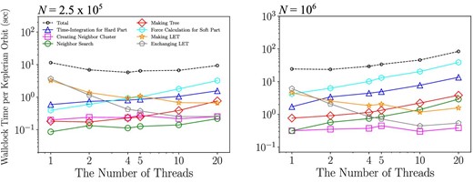
$Wallclock time taken for each procedure per Keplerian orbit as a function of the number of MPI processes per node in the cases of 1.25 × 105 (left) and 106 (right) particles. We used θ = 0.5, Δt = 1/64, $\tilde{R}_{\rm cut}=2$, and 640 CPU cores (i.e., the number of MPI processes is 640 divided by the number of threads). (Color online)$

Fig. 7.

Wallclock time taken for each procedure per Keplerian orbit as a function of the number of MPI processes per node in the cases of 1.25 × 10⁵ (left) and 10⁶ (right) particles. We used θ = 0.5, Δt = 1/64, |$\tilde{R}_{\rm cut}=2$|⁠, and 640 CPU cores (i.e., the number of MPI processes is 640 divided by the number of threads). (Color online)

Open in new tab Download slide

3.2.2 Systems with mass spectrum

In this section we present the results of calculations with particles with a mass spectrum in order to evaluate the behavior of GPLUM at the late stage of planetary formation. As the initial model we used the output snapshot at 9998 years of integration from the initial model described in the previous section. The minimum, average, and maximum masses are 2.00 × 10²¹, 5.30 × 10²¹, and 8.46 × 10²⁴ g, respectively. The number of particles is 377740. We used the enhancement factor for particle radius of f = 1.

Figure 8 shows the maximum energy error over 10 Kepler times as a function of |$\Delta t/\tilde{R}_{\rm cut,0}$| and Δt in the case of shared, individual, and individual and random velocity cut-off schemes. Here, θ = 0.1. If we compare the values of |$\Delta t/\tilde{R}_{\rm cut,0}$| itself, it seems the individual cut-off scheme requires a rather small value of Δt, but when the term for the random velocity is included, we can see that the energy error is essentially independent of |$\tilde{R}_{\rm cut,0}$|⁠. Since the energy error, which depends on |$\Delta t/\tilde{R}_{\rm cut,0}$| when |$\Delta t/\tilde{R}_{\rm cut,0}\gtrsim 10^{-2}$| in the shared and individual cut-off schemes, does not appear when the random velocity cut-off scheme is used, this error seems to cause the cut-off radius to not be set sufficiently larger than v_ranΔt. The energy error almost does not depend on Δt and |$\tilde{R}_{\rm cut,0}$| in the case of the random velocity cut-off scheme. Therefore, we can use larger Δt and smaller |$\tilde{R}_{\rm cut,0}$| to reduce the time of simulation while maintaining accuracy.

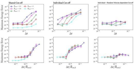
$Maximum energy error over five Keplerian orbits as a function of $\Delta t/\tilde{R}_{\rm cut,0}$ (top) and Δt (bottom) in the case of θ = 0.1, shared cut-off (left), individual cut-off (center), and individual and random velocity-dependent cut-off (right). (Color online)$

Fig. 8.

Maximum energy error over five Keplerian orbits as a function of |$\Delta t/\tilde{R}_{\rm cut,0}$| (top) and Δt (bottom) in the case of θ = 0.1, shared cut-off (left), individual cut-off (center), and individual and random velocity-dependent cut-off (right). (Color online)

Open in new tab Download slide

Figure 9 shows the wallclock time for the integration over one Kepler time and its breakdown as a function of |$\tilde{R}_{\rm cut,0}$| in the case of θ = 0.5, Δt = 1/64. In the case of the shared cut-off scheme, the calculation cost increases quickly as we increase |$\tilde{R}_{\rm cut,0}$|⁠. On the other hand, from figure 8 we can see that for Δt = 1/64, we need |$\tilde{R}_{\rm cut,0} \ge 1$| in the case of the shared cut-off scheme to achieve reasonable accuracy.

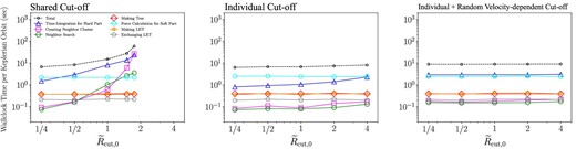
$Wallclock time taken for simulations per Keplerian orbit as functions of $\tilde{R}_{\rm cut}$ in the case of θ = 0.5, Δt = 1/64, shared cut-off (left), individual cut-off (center), and individual and random velocity-dependent cut-off (right). (Color online)$

Fig. 9.

Wallclock time taken for simulations per Keplerian orbit as functions of |$\tilde{R}_{\rm cut}$| in the case of θ = 0.5, Δt = 1/64, shared cut-off (left), individual cut-off (center), and individual and random velocity-dependent cut-off (right). (Color online)

Open in new tab Download slide

For individual cut-off schemes with and without the random velocity term, the total calculation cost is almost independent of |$\tilde{R}_{\rm cut,0}$|⁠, and in the case of the scheme with the random velocity term, the total energy error is also well conserved for all values of |$\tilde{R}_{\rm cut,0}$|⁠. Thus, we can see that individual cut-off schemes with a random velocity term are more efficient compared to the shared cut-off schemes for realistic distribution of particle mass and random velocity.

Figure 10 shows the average number of neighbors, 〈n_b〉, and the number of particles in the largest neighbor cluster, n_{b, max}, as functions of |$\tilde{R}_{\rm cut,0}$| in the case of θ = 0.5, Δt = 1/64. The average number of neighbors is roughly proportional to |$\tilde{R}_{\rm cut,0}^3$|⁠, while almost independent of |$\tilde{R}_{\rm cut,0}^3$| for the case of the individual cut-off with random velocity term. This, of course, means that for most particles their neighbor is determined by the random velocity term, and only the neighbors of the most massive particles are affected by the individual term. This effect on the neighbors of the most massive particles is very important in maintaining high accuracy and high efficiency.

$Average number of neighbors for each particle, 〈nb〉, (left) and the number of particles in the largest neighbor cluster, nb, max, (right) as functions of $\tilde{R}_{\rm cut}$ in the case of θ = 0.5, Δt = 1/64. The dotted line in the left panel represents the slope of $\langle n_b\rangle \propto \tilde{R}_{\rm cut,0}^3$. (Color online)$

Fig. 10.

Average number of neighbors for each particle, 〈n_b〉, (left) and the number of particles in the largest neighbor cluster, n_{b, max}, (right) as functions of |$\tilde{R}_{\rm cut}$| in the case of θ = 0.5, Δt = 1/64. The dotted line in the left panel represents the slope of |$\langle n_b\rangle \propto \tilde{R}_{\rm cut,0}^3$|⁠. (Color online)

Open in new tab Download slide

3.2.3 Long-term simulations

In this section we present the result of long-term integration of up to 20000 yr. We included the gas drag according to the model in Adachi, Hayashi, and Nakazawa (1976) for the MMSN model, and we used the simple fragmentation model with a = 0.3, b = 0.1 in the case of the individual cut-off with random velocity term. We used parameters of θ = 0.5, Δt = 1/64, |$\tilde{R}_{\rm cut,0}=3$|⁠, and f = 3. We had to stop the simulation with the shared time step since it had become too slow.

Figure 11 shows the energy error as a function of time. We can see that for the first 1000 yr all the schemes show similar behavior. However, the error of the run with the shared cut-off scheme starts to grow by 2000 yr, and then the calculation becomes too slow. The error of the run with the individual cut-off without the random velocity term also starts to grow by 6000 yr. When the random velocity term is included, the error remains small even after 20000 yr. In the case of shared cut-off, it is considered that the energy error due to random velocity appears earlier since the cut-off radius is larger.

Fig. 11.

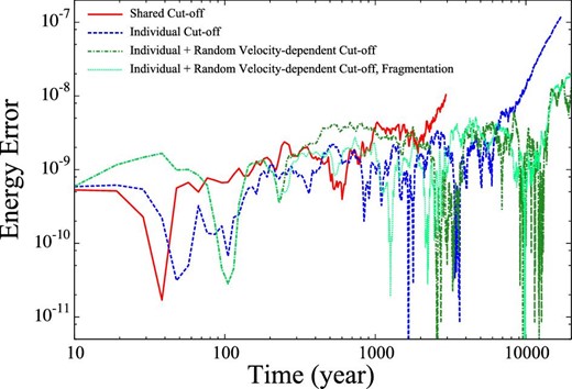
Evolution of energy error for long-term simulations in the case of θ = 0.5, Δt = 1/64, shared cut-off with perfect accretion (solid red), individual cut-off with perfect accretion (solid blue), individual and random velocity-dependent cut-off with perfect accretion (solid green), and individual and random velocity-dependent cut-off with fragmentation (dashed light green). (Color online)

Open in new tab Download slide

Note that this result is for one particular choice of the accuracy parameters and it is possible to improve the error of, for example, the shared cut-off scheme by reducing the soft time step. On the other hand, the individual cut-off scheme with the random velocity term can keep the error small even after the most massive particle grows by three orders of magnitude in mass (see figure 13). Thus, we conclude that the the individual cut-off scheme with the random velocity term can be reliably used for long-term simulations.

Figure 12 shows the wallclock time as a function of simulation time. The increase of the calculation time of the shared cut-off scheme is faster than linear, while that of the individual cut-off schemes is slower, because of the decrease in the number of particles. At the time of the first snapshot (10 yr), because the mass of the largest body already reaches about nine times the initial mass, the mean cut-off radius in the case of shared cut-off is about twice as large as for individual cut-off. This is the reason why the calculation speed in the case of shared cut-off is slower than the individual case from the beginning of the simulation.

Fig. 12.

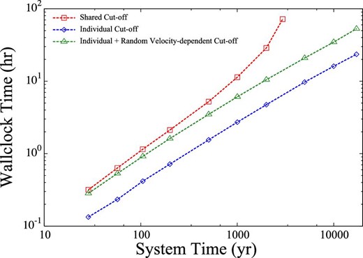
Wallclock time taken for long-term simulations until time t as a function of t in the case of shared cut-off (red) and individual cut-off (blue). (Color online)

Open in new tab Download slide

Figure 13 shows the evolution of the number of particles and the mass of the most massive particle. We can see that the time evolutions obtained using different cut-off schemes are practically identical.

Fig. 13.

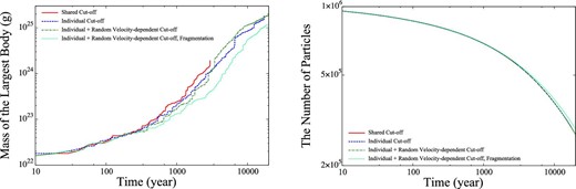
Evolution of number of particles (left) and mass of the largest body (right) for long-term simulations in the case of θ = 0.5, Δt = 1/64, shared cut-off with perfect accretion (solid red), individual cut-off with perfect accretion (solid blue), individual and random velocity-dependent cut-off with perfect accretion (solid green), and individual and random velocity-dependent cut-off with fragmentation (dashed light green). (Color online)

Open in new tab Download slide

Figures 14 and 15 show the mass distributions and rms random velocities of particles at years 1499 and 2502. The result does not depend on the choice of the cut-off scheme. Thus, we can conclude that the choice of the cut-off scheme does not affect the dynamics of the system.

Fig. 14.

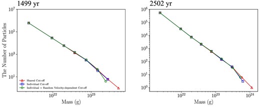
Mass distributions of particles in the case of shared cut-off (red) and individual cut-off (blue) with perfect accretion at 1499 yr (left) and 2502 yr (right). We plot the distribution at 2435 yr in the case of shared cut-off instead of at 2502 yr since the simulation was not performed until 2502 yr in that case. (Color online)

Open in new tab Download slide

Fig. 15.

Distribution of rms of orbital eccentricities (top) and inclinations (bottom) of particles as a function of mass in the case of shared cut-off (red), individual cut-off (blue), and individual and random velocity-dependent cut-off with perfect accretion (green) with perfect accretion at 1499 yr (left) and 2502 yr (right). We plot the distribution at 2435 yr in the case of shared cut-off instead of 2502 yr since the simulation was not performed until 2502 yr in that case. The error bars show 70% confidence intervals.

Open in new tab Download slide

Figure 16 shows the average number of neighbors, 〈n_b〉, and the number of particles in the largest neighbor cluster, |$n_{b,\rm max}$|⁠. Because the mass of the largest body already reaches about nine times the initial mass at 10 yr, the average number of neighbors in the case of shared cut-off is larger than in the case of individual cut-off from the beginning of the simulation. The average number of neighbors 〈n_b〉 for the shared cut-off scheme increases with time, since the shared cut-off radius is determined by the mass of the most massive particle. On the other hand, that for individual cut-off, with and without the random velocity term, initially decreases partly because the total number of particles decreases due to collisions, and partly because of the increase in the inclination of particles. However, after around 5000 yr, 〈n_b〉 for the scheme with random velocity term starts to increase due to the increase in the random velocity. This increase does not result in a notable increase in the calculation time, as can be seen in figure 12. This is simply because 〈n_b〉 is still very small.

Fig. 16.

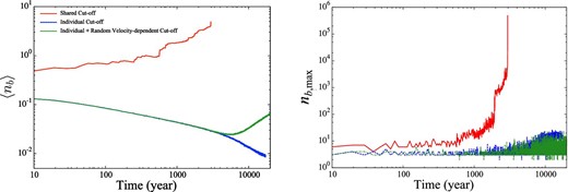
Evolution of the average number of neighbors for each particle, 〈n_b〉, (left) and the number of particles in the largest neighbor cluster, n_{b, max}, (right) in the case of shared cut-off (red), individual cut-off (blue), and individual and random velocity-dependent cut-off with perfect accretion (green).

Open in new tab Download slide

In the case of the shared cut-off scheme, |$n_{b,\rm max}$| approached the total number of particles when the calculation was halted. This increase in the size of the cluster is of course the reason why the calculation became very slow. This means that the neighbor cluster showed percolation, which is expected to occur if 〈n_b〉 is larger than the critical value of order unity. When percolation of the neighbor cluster occurs, our current implementation falls back to the O(N²) direct Hermite scheme on a single MPI process. Thus, it is necessary to avoid percolation, and that means we should keep 〈n_b〉 ≪ 1.

4 Discussion and conclusion

We have presented the implementation and performance of GPLUM, parallel N-body simulation code based on the |$\rm P^3T$| scheme. The main difference from the previous implementation of the parallel |$\rm P^3T$| scheme (Iwasawa et al. 2017) is that we introduced an individual cut-off radius which depends both on the particle mass and the local velocity dispersion. The dependence on the mass is necessary to handle systems with a wide range of mass spectrum, and the the local velocity dispersion dependence is necessary to maintain accuracy when the velocity dispersion becomes high. With this new treatment of the cut-off radius, GPLUM can follow a planetary formation process in which the masses of the planetesimals grow by many orders of magnitude without a significant increase in the calculation time.

We have confirmed that the use of the individual cut-off has no effect on the result, and that accuracy is improved and the calculation time is shortened compared to the shared cut-off scheme.

The parallel performance of GPLUM is reasonable for up to 1000 cores. On the other hand, there are systems with much larger numbers of cores. In particular, the Fugaku supercompuer, which is currently the fastest computer in the world, has around eight million cores. In order to make efficient use of such machines, the scalability of GPLUM should be further improved.

Due to both the distribution of calculation and the increase of communication due to parallelization, there are optimum values for the numbers of parallel MPI and OpenMP. It should be noted that the optimum values differ depending on the system.

As discussed in sub-subsection 3.2.1, currently the limiting factor for the parallel performance is the time for LET construction, which can be reduced by several methods (Iwasawa et al. 2019). We plan to apply such methods and improve the parallel performance.

GPLUM is freely available for all those who are interested in particle simulations. The source code is hosted on the GitHub platform and can be downloaded from their site;¹ it has the MIT license.

Acknowledgements

This work was supported by MEXT as “Program for Promoting Researches on the Supercomputer Fugaku” (Toward a unified view of the universe: from large scale structures to planets). This work uses HPCI shared computational resources hp190060 and hp180183. The simulations in this paper were carried out on a Cray XC50 system at the Centre for Computational Astrophysics (CfCA) of the National Astronomical Observatory of Japan (NAOJ) and a Cray XC40 system at the Academic Center for Computing and Media Studies (ACCMS) of Kyoto University. Test simulations were also carried out on Shoubu ZettaScaler-1.6 at the Institute of Physical and Chemical Research (RIKEN). We acknowledge the contribution of Akihisa Yamakawa, who developed an early version of the parallel |$\rm P^3T$| code.

Footnotes

1

https://github.com/YotaIshigaki/GPLUM.

References

Aarseth

S. F.

1963

,

MNRAS

,

126

,

223

Crossref

Search ADS

Adachi

I.

,

Hayashi

C.

,

Nakazawa

K.

1976

,

Prog. Theor. Phys.

,

56

,

1756

Crossref

Search ADS

Barnes

J.

,

Hut

P.

1986

,

Nature

,

324

,

446

Crossref

Search ADS

Chambers

J. E.

2013

,

Icarus

,

224

,

43

Crossref

Search ADS

Fujii

M.

,

Iwasawa

M.

,

Funato

Y.

,

Makino

J.

2007

,

PASJ

,

59

,

1095

Crossref

Search ADS

Hayashi

C.

1981

,

Prog. Theor. Phys. Suppl.

,

70

,

35

Crossref

Search ADS

Ida

S.

,

Makino

J.

1992

,

Icarus

,

96

,

107

Crossref

Search ADS

Ikoma

M.

,

Emori

H.

,

Nakazawa

K.

1998

,

J. Phys. Cond. Matt.

,

10

,

11537

Crossref

Search ADS

Iwasawa

M.

et al.

2019

,

arXiv:1907.02289

Iwasawa

M.

,

Oshino

S.

,

Fujii

M. S.

,

Hori

Y.

2017

,

PASJ

,

69

,

81

Crossref

Search ADS

Iwasawa

M.

,

Tanikawa

A.

,

Hosono

N.

,

Nitadori

K.

,

Muranushi

T.

,

Makino

J.

2016

,

PASJ

,

68

,

54

Crossref

Search ADS

Kokubo

E.

,

Ida

S.

1996

,

Icarus

,

123

,

180

Crossref

Search ADS

Kokubo

E.

,

Ida

S.

1998

,

Icarus

,

131

,

171

Crossref

Search ADS

Kokubo

E.

,

Ida

S.

2002

,

ApJ

,

581

,

666

Kominami

J.

,

Daisaka

H.

,

Makino

J.

,

Fujimoto

M.

2016

,

ApJ

,

819

,

30

Crossref

Search ADS

Makino

J.

1991

,

ApJ

,

369

,

200

Crossref

Search ADS

Makino

J.

,

Fukushige

T.

,

Koga

M.

,

Namura

K.

2003

,

PASJ

,

55

,

1163

Crossref

Search ADS

Makino

J.

,

Kokubo

E.

,

Taiji

M.

1993

,

PASJ

,

45

,

349

Minton

D. A.

,

Levison

H. F.

2014

,

Icarus

,

232

,

118

Crossref

Search ADS

Mizuno

H.

1980

,

Prog. Theor. Phys.

,

64

,

544

Crossref

Search ADS

Mizuno

H.

,

Nakazawa

K.

,

Hayashi

C.

1978

,

Prog. Theor. Phys.

,

60

,

699

Crossref

Search ADS

Nitadori

K.

,

Makino

J.

,

Abe

G.

2006

,

arXiv:astro-ph/0606105

Oshino

S.

,

Funato

Y.

,

Makino

J.

2011

,

PASJ

,

63

,

881

Crossref

Search ADS

Sugimoto

D.

,

Chikada

Y.

,

Makino

J.

,

Ito

T.

,

Ebisuzaki

T.

,

Umemura

M.

1990

,

Nature

,

345

,

33

Crossref

Search ADS

This article is published and distributed under the terms of the Oxford University Press, Standard Journals Publication Model (https://dbpia.nl.go.kr/journals/pages/open_access/funder_policies/chorus/standard_publication_model)

Download all slides

Month:	Total Views:
May 2021	29
June 2021	6
July 2021	12
August 2021	3
October 2021	8
November 2021	1
December 2021	3
January 2022	1
February 2022	2
March 2022	3
April 2022	2
May 2022	12
June 2022	4
July 2022	7
August 2022	5
October 2022	1
November 2022	1
December 2022	4
March 2023	3
April 2023	5
May 2023	20
June 2023	13
July 2023	25
August 2023	25
September 2023	23
October 2023	19
November 2023	8
December 2023	13
January 2024	30
February 2024	25
March 2024	20
April 2024	10
May 2024	10
June 2024	6
July 2024	34
August 2024	10
September 2024	13
October 2024	19
November 2024	7
December 2024	6
January 2025	7
February 2025	13
March 2025	18
April 2025	11
May 2025	4

Article Contents

Particle–particle particle–tree code for planetary system formation with individual cut-off method: GPLUM

Abstract

1 Introduction

2 Numerical method

2.1 Basic equations

2.1.1 The P³T scheme

2.1.2 The P³T scheme with individual cut-off

2.1.3 The P³T scheme with Hill radius and random velocity dependent cut-off

2.2 Data structure and time-integration procedure

2.3 Neighbor cluster creation procedure

2.4 Treatment of collisions

2.4.1 Perfect accretion model

2.4.2 Implementation of fragmentation

2.4.3 Fragmentation models

3 Result

3.1 Initial conditions and simulation parameters

3.2 Accuracy and performance

3.2.1 Equal-mass systems

3.2.2 Systems with mass spectrum

3.2.3 Long-term simulations

4 Discussion and conclusion

Acknowledgements

Footnotes

References

Citations

Views

Altmetric

Email alerts

Astrophysics Data System

Citing articles via

Latest

Most Read

Most Cited

Article Contents

Particle–particle particle–tree code for planetary system formation with individual cut-off method: GPLUM

Abstract

1 Introduction

2 Numerical method

2.1 Basic equations

2.1.1 The P3T scheme

2.1.2 The P3T scheme with individual cut-off

2.1.3 The P3T scheme with Hill radius and random velocity dependent cut-off

2.2 Data structure and time-integration procedure

2.3 Neighbor cluster creation procedure

2.4 Treatment of collisions

2.4.1 Perfect accretion model

2.4.2 Implementation of fragmentation

2.4.3 Fragmentation models

3 Result

3.1 Initial conditions and simulation parameters

3.2 Accuracy and performance

3.2.1 Equal-mass systems

3.2.2 Systems with mass spectrum

3.2.3 Long-term simulations

4 Discussion and conclusion

Acknowledgements

Footnotes

References

Citations

Views

Altmetric

Email alerts

Astrophysics Data System

Citing articles via

Latest

Most Read

Most Cited

This Feature Is Available To Subscribers Only

2.1.1 The P³T scheme

2.1.2 The P³T scheme with individual cut-off

2.1.3 The P³T scheme with Hill radius and random velocity dependent cut-off