


Abstract
The radio nebula W 50 is a unique object interacting with the jets of the microquasar SS 433. The SS 433/W 50 system is a good target for investigating the energy of cosmic-ray particles accelerated by galactic jets. We report observations of the radio nebula W 50 conducted with the National Science Foundation’s Karl G. Jansky Very Large Array in the L band (1.0–2.0 GHz). We investigate the secular change of W 50 on the basis of the observations in 1984, 1996, and 2017, and find that most of its structures were stable for 33 yr. We revise the upper-limit velocity of the eastern terminal filament by half to 0.023 c, assuming a distance of 5.5 kpc. We also analyze observational data from the Arecibo Observatory 305 m telescope and identify the H i cavity around W 50 in the velocity range 33.77–55.85 km s−1. From this result, we estimate the maximum energy of the cosmic-ray protons accelerated by the jet terminal region to be above 1015.5 eV. We also use the luminosity of the gamma-rays in the range 0.5–10 GeV to estimate the total energy of accelerated protons below 5.2 × 1048 erg.
1 Introduction
The microquasar SS 433 is one of the most famous jet sources in our galaxy. Its outstanding feature is ejection of two-sided precessing jets. The jet velocity is 0.26 c and the precession period is 162 d (Abell & Margon 1979; Margon 1984; Margon & Anderson 1989; Davydov et al. 2008). The half-opening angle of the precessing jets is 20° (Margon 1984). The helical shape of the jets is believed to be broken down within the subparsec scale, and the hollow jets proceed for dozens of parsecs (Brinkmann et al. 2007; Monceau-Baroux et al. 2015; Panferov 2017).
SS 433 is located at the geometric center of the large radio nebula W 50. The nebula consists of one spherical shell and two elongated structures called “wings” (Geldzahler et al. 1980; Downes et al. 1981a, 1981b, 1986; Dubner et al. 1998). Because the jet axis is well aligned with the direction of the wings, the jet and nebula are considered to have some physical association. Elston and Baum (1987) first observed W 50 with the historical Very Large Array (VLA) with a high resolution of 60″, and suggested that the wings were formed by the ram pressure of the SS 433 jet on the W 50 shell. Dubner et al. (1998) carried out high-sensitivity mosaic observation of W 50 with the VLA at 1.4 GHz and succeeded in resolving the complex structures with a high dynamic range. In recent years, wide-band and high-sensitivity full-Stokes observation has enabled detailed polarization analysis (Farnes et al. 2017). Farnes et al. (2017) identified a large-scale rotation measure gradient across the spherical shell in the east–west direction and across the eastern edge of the wing in the north–south direction using Australia Telescope Compact Array (ATCA) data at 1.1–3.1 GHz. Sakemi et al. (2018) focused on the eastern edge of the wing and identified the helical magnetic fields coiling around the eastern wing. The latest radio continuum observation was reported by Broderick et al. (2018). They observed W 50 with the Low-Frequency Array (LOFAR) over the frequency range 115–189 MHz. The morphology of W 50 observed at low frequency showed agreement with the high-frequency observation. They found that only the flux of the eastern wing was lower than the value predicted by the power-law spectrum, probably because of the foreground free–free absorption.
One of the outstanding issues of the SS 433/W 50 system is the origin of the spherical shell of W 50. Two major models are (i) a wind bubble from a binary companion of SS 433, a progenitor star, or an accretion disk with a mass accretion rate exceeding the Eddington limit (Konigl 1983; Asahina et al. 2014), and (ii) a supernova remnant (SNR) originating from SS 433 (Downes et al. 1986). A combination of these models is also possible (Ciotti & D’Ercole 1989; Tenorio-Tagle et al. 1991; Rozyczka et al. 1993). However, both scenarios have the same difficulty: although it takes a long time for the shell radius to increase by about 50 pc, the shell is still bright. Furthermore, the mechanism of formation of the wings by the jets has not yet been determined. Goodall, Blundell, and Bell Burnell (2011b) estimated the upper velocity of the eastern terminal region of the jet as 0.0405 c (12142 km s−1) using radio observation datasets for the 12 years between 1984 and 1996. They concluded that a continuous, non-multi-episodic jet could not be decelerated to a velocity below this upper limit because the surrounding interstellar medium (ISM) has a low density of 0.1–1 particles cm−3, and intermittent jets are required for the morphology of W 50, including the wings (Goodall et al. 2011a). However, Panferov (2017) suggested that a continuous jet could be decelerated by ambient matter considering viscosity, which means that a continuous jet could construct the wing structures.
Recently, another formation scenario for W 50 has been proposed: only jets from SS 433 can produce the whole morphology of W 50 (Ohmura et al. 2021). Some active galactic nuclei (AGNs) show a shell-like structure with wings (Roberts et al. 2015), and some numerical simulations have succeeded in reproducing this unique morphology (Gaibler et al. 2009; Hodges-Kluck & Reynolds 2011; Rossi et al. 2017). A similar model can be applied to galactic X-ray binary jets considering this scaling law. Ohmura et al. (2021) suggested that the morphology of W 50 could be reproduced by low-density and continuous jets on the basis of magnetohydrodynamic simulation. Their results imply that we should introduce a new hypothesis for the origin of the SS 433/W 50 system.
In recent decades, microquasar jets have been considered as candidates for accelerators of high-energy cosmic-ray particles above 1015 eV (Romero & Vila 2008; Pepe et al. 2015; Cooper et al. 2020; Sudoh et al. 2020). The SS 433/W 50 system is an appropriate target for observing cosmic-ray particle acceleration by galactic jets. X-ray observations have identified emission from the SS 433 jet (Kotani et al. 1996; Brinkmann et al. 1996, 2007; Safi-Harb & Ögelman 1997; Safi-Harb & Petre 1999). The X-ray hotspot is located near the border between the spherical shell and the eastern wing, and it has both thermal and non-thermal components. TeV-scale gamma-ray emission has been identified at the same position by Abeysekara et al. (2018), who suggested that the origin of the emission was the interaction between cosmic microwave background photons and accelerated electrons through inverse Compton scattering; this is called the leptonic scenario. Sudoh, Inoue, and Khangulyan (2020) also supported the leptonic scenario theoretically. However, Kimura, Murase, and Mészáros (2020) suggested the hadronic scenario, whereby interaction between cosmic-ray protons and interstellar protons can also explain the TeV gamma-ray emission.
GeV-scale gamma-ray emission has also been detected by analyzing Fermi-LAT data over 10 years, and there is still debate on whether it has the same origin as TeV gamma-ray emission. Sun et al. (2019) suggested that the position of the GeV gamma-ray emission is different from that of the TeV gamma-rays and is located in the northern area of the spherical shell of W 50. They considered the origin of this emission to be the interaction between the spherical shell and the surrounding ISM (hadronic scenario). Li et al. (2020) also analyzed the Fermi-LAT data while considering the influence of the nearby pulsar PSR J1907+0602, and they detected a GeV gamma-ray excess in the northeast area of the spherical shell. They found a periodic variation of this emission with the precession period of the SS 433 jet. However, Fang, Charles, and Blandford (2020) suggested that the position of the GeV gamma-ray emission is the same as that of the TeV gamma-rays, and that these emissions are induced by the SS 433 jet. Identifying the origin of the GeV gamma-ray emission is necessary for understanding the cosmic-ray particle acceleration by the SS 433/W 50 system.
The SS 433/W 50 system also has another candidate for inducing cosmic-ray particle acceleration at the eastern edge of W 50. This candidate is a filamentary structure that is bright in the radio and X-ray bands and perpendicular to the SS 433 jet axis (Elston & Baum 1987; Brinkmann et al. 2007). In this paper, we call this filamentary structure the “eastern terminal filament” (ETF). Because the SS 433 jet is believed to reach the position of the ETF, a terminal shock should form in this region. This makes it possible for cosmic-ray particles to be accelerated by the terminal shock. Although no gamma-ray emission has ever been observed here, a future high-sensitivity telescope like the Cherenkov Telescope Array (CTA) may detect it. Verifying cosmic-ray particle acceleration in this region is essential for comprehensively understanding acceleration by galactic jets.
It is difficult to determine the distance of the SS 433/W 50 system from us. The distance has been estimated at 5.5 kpc on the basis of a kinematic model derived from optical line observation and radio images of the precessing jet (Eikenberry et al. 2001; Blundell & Bowler 2004; Blundell et al. 2018). This is different from the distance of ∼4.6 kpc estimated from parallax observation of the binary companion star with Gaia Data Release 2 (Gaia Collaboration 2018). Recently, the distance has been newly estimated as 8.5 kpc using Gaia Early Data Release 3 (EDR3) (Gaia Collaboration 2020). Therefore, there is a large uncertainty in the distance of SS 433 and W 50. Because EDR3 still has some calibration issues, we do not consider its value for the distance in this paper (Maíz Apellániz et al. 2021).
The other method for estimating the distance is to identify the ISM interacting with W 50. If we assume the velocity field of our galaxy, we can investigate ISM distances on the basis of their line-of-sight velocities. Many studies in recent decades have suggested a relation between W 50 and the ISM. Dubner et al. (1998) found the surrounding H i gas at the systematic radial velocity vLSR = 42 km s−1. The H i gas in their observation seemed to have a cavity-like structure surrounding W 50; however, a spatial coincidence with W 50 was hard to ascertain owing to a low angular resolution of 21′. Furthermore, while the velocity center of the H i cavity was revealed, the velocity range of the cavity was still unknown. Lockman, Blundell, and Goss (2007) detected the H i absorption line of SS 433 at a velocity of 75 km s−1 and identified the H i emission at the same velocity, which shows good spatial coincidence with the western wing. Molecular clouds were also detected around W 50. For example, Yamamoto et al. (2008) found molecular clouds whose velocity range was 42–56 km s−1. These clouds are well aligned close to the SS 433 jet axis. Liu et al. (2020) observed a few clouds detected by Yamamoto et al. (2008) and suggested that one of them was within the western wing of W 50. Su et al. (2018) found other clouds near the western wing and a straight extension of the eastern wing in the velocity range 73–84 km s−1. Thus, the intrinsic velocity range of the ISM interacting with W 50 has not yet been identified. Because of the velocity variation of the candidate ISM, it is difficult to determine the distance of W 50 more precisely than as being between 3.0 and 5.5 kpc. Determining the intrinsic velocity is also important for identifying the origin of the gamma-ray emission induced by the interaction with cosmic-ray protons and estimating their total energy.
In this paper, our purpose is to investigate the influence of the SS 433 jet on the morphology of W 50. We further aim to specify the velocity range of the interacting ISM. Therefore, we compare the radio continuum images over 33 yr, including the latest observation with the NSF’s Karl G. Jansky Very Large Array (VLA) in the L band (1.0–2.0 GHz) in 2017. We also determine the distribution of the H i gas around W 50 using archived survey data. From these results, we estimate the maximum energy of accelerated cosmic-ray particles in the SS 433 jet terminal. Finally, we estimate the total energy of cosmic-ray protons associated with the GeV gamma-ray emission, assuming interaction with the H i gas. The paper is structured as follows: In section 2, we describe the observational data and the method of calibration; in section 3, we show the results of our analysis; in section 4, we provide a discussion; and in section 5 we provide our conclusion.
2 Observation and calibration
2.1 Radio continuum
2.1.1 Observation in 2017
W 50 was observed with the VLA in the L band on 2017 April 25 (project code: 17A-291; PI: G. M. Dubner). The array was in the D configuration during the observations. W 50 extends over 1° × 2° in size; however, the primary beam size is only 28′ at 1.5 GHz. Then, a 58-pointing mosaic was used to cover all of the structures. The pointing separation was 15′. The pointings satisfied Nyquist sampling at 1.4 GHz. Each pointing was observed twice in snapshots of 152 s.
The data were calibrated and imaged using the Common Astronomy Software Applications (casa) package following standard procedures. J1331+3030 and J1859+1259 are the flux density calibrator and the phase calibrator, respectively. L-band observations are severely affected by radio frequency interference (RFI). We checked the frequency channel affected by RFI and flagged the data below 1.327 GHz, between 1.520 and 1.711 GHz, and above 1.904 GHz.
Diffuse emission from W 50 is hidden by significant artifacts because some bright sources such as SS 433 exist within the observation field. To reduce the sidelobe level, we first carried out clean deconvolution of the image using the tclean task while masking only 15 bright point sources, including SS 433. We repeated tclean until all the peak fluxes reached five times the rms noise level. The artifacts seemed improved at this stage. After tclean was performed on the bright point sources, we performed tclean for other radio sources in the target field including W 50. Because W 50 has extended structures, we applied the multi-scale, multi-term multi-frequency synthesis algorithm, setting nterms = 1 (Rau & Cornwell 2011). The phase center was at |${19^{\rm h}12^{\rm m}17^{\rm s}}$|, |${4^{\circ}58^{\prime }00^{\prime \prime }}$|. Images were made using Briggs weighting with robust = 0.5. We also set a low loop gain, 0.005, in order not to miss diffuse and faint emission. Finally, the image had a resolution of 53″ × 43″ with a position angle of −47|${{_{.}^{\circ}}}$|9 (0.8 pc × 0.6 pc at a distance of 3.0 kpc and 1.4 pc × 1.1 pc at a distance of 5.5 kpc).
In addition to the full-frequency image, we made an image whose frequency range accords with the observations in 1984 and 1996 to compare the structures in detail. The image was constructed through the same process as for the full-frequency image. We smoothed the final image with a beam size of 60″ × 60″ (0.9 pc at a distance of 3.0 kpc and 1.6 pc at a distance of 5.5 kpc) using the imsmooth task to equalize the beam size between all observation periods.
2.1.2 Calibration and imaging of past observation datasets
To examine variations of structures of W 50 over 33 yr, we also calibrated and imaged the observation data in 1984 and 1996. W 50 was observed with the VLA at 1.465 GHz on 1984 August 12 and 13 (Elston & Baum 1987). The array configuration was also D, and nine pointings were used. W 50 was also observed with the VLA at 1.465 GHz on 1996 August 19 (Dubner et al. 1998). The array configuration was also D, and mosaicking was carried out with 58 pointings. We calibrated this dataset with casa, following standard procedures. The image was constructed through the same process as for the full-frequency image of the 2017 observation. We smoothed the final images with a convolved beam size of 60″ × 60″ using the imsmooth task.
2.2 The GALFA-H i survey
To search the interstellar medium associated with W 50, we used the Galactic Arecibo L-band Feed Array H i (GALFA-H i) survey data (Peek et al. 2011). The survey was carried out with the Arecibo Observatory 305 m telescope. Its angular resolution was 4′, and the velocity resolution was 0.18 km s−1. The velocity coverage was −700 km s−1 < VLSR < +700 km s−1. Its typical noise level was 80 mK rms in an integrated 1 km s−1 channel.
3 Results
3.1 Comparison of the structures of W 50 over 33 yr
3.1.1 Astrometric error
To discuss detailed motions using multiple-period observations, it is important to determine the astrometric error. We used the alignment accuracy of point sources that did not relocate during the observation interval. We first checked offsets in the position of the flux calibrator 3C 286 by comparing the reference position that the observatory offers. 3C 286 was imaged using the casa task tclean. After tclean, we smoothed with a convolved beam size of 60″ × 60″ using ther imsmooth task. We fitted a Gaussian function to determine the position of 3C 286. Finally, we obtained the offset values by determining the difference from the reference position. The results are listed in table 1. The position accuracy in 1984 is poor compared with the 1996 and 2017 observations, and the cause might be the weather or imperfect correction of the antenna position.
Position offset of the flux calibrator.*
| Year | Right ascension (″) | Declination (″) |
|---|---|---|
| 1984 | +8.74524 | −7.55885 |
| 1996 | −0.01476 | −0.01885 |
| 2017 | −0.01476 | +0.00115 |
| Year | Right ascension (″) | Declination (″) |
|---|---|---|
| 1984 | +8.74524 | −7.55885 |
| 1996 | −0.01476 | −0.01885 |
| 2017 | −0.01476 | +0.00115 |
Comparison with the position of 3C 286 on the list of VLA calibrators. The position is RA (J2000.0) = |${13^{\rm h}31^{\rm m}08{_{.}^{\rm s}}287984}$|, Dec (J2000.0) = +30°|${30^{\prime }32^{^{\prime\prime}_{.}}958850}$|.
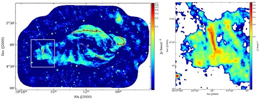
We also checked the positions of bright radio sources in the target field. The sources are shown in the left panel of figure 1 with cyan boxes. We calculated the position offsets of these sources between 2017 and 1996 (red), 1996 and 1984 (blue), and 2017 and 1984 (green; right panel of figure 1). Most sources have no offset; however, the positions of some bright sources are slightly different between observation periods. The numbers in the plot correspond to the source numbers in the left panel. Their offset values coincide with the pixel size of the total intensity maps, ∼8″.
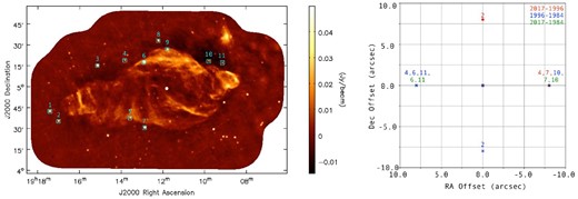
(Left) Total intensity map of W 50 observed in 2017. The cyan boxes show the positions of bright radio sources used to assess the accuracy of position determination. (Right) Offsets of the positions of bright radio sources between observation periods. Comparisons between 2017 and 1996, 1996 and 1984, and 2017 and 1984 are represented with a red circle, blue cross, and green plus, respectively. We label only the sources that have offsets.
Discussing the motion of a radio component on a small scale requires caution and sometimes causes misunderstanding. Therefore, we adopt the largest offset of 3C 286 in 1984, |${8{^{\prime \prime}_{.}}74524}$|, as the astrometric error.
3.1.2 Comparison of total intensity distributions
To determine whether the morphology of W 50 changed over 33 yr, we compared the observations in 1984, 1996, and 2017. We made the total intensity map of each observation period using the same tclean setup: phase reference, map size, grid size, and weighting (figures 2, 3, and 4). Furthermore, we equalized the beam size to be 60″ × 60″. After that, we found the peak positions of the bright filaments.
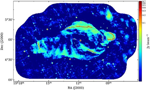
Positions of the filamentary structures observed in 2017. The back image is a total intensity map at 1.440–1.490 GHz. The beam size is 60″ × 60″.
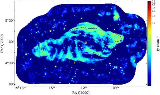
Similar to figure 2, but for the observation in 1996.
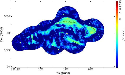
Similar to figure 2, but for the observation in 1984.
The green, blue, and red curves in figure 5 represent the peak positions of the characteristic filaments observed in 1984, 1996, and 2017, respectively. The bright filaments do not show significant motions above the astrometric error during the 33 yr. Remarkably, the filament perpendicular to the jet axis, the ETF, seems to remain stationary even though it should be influenced by the SS 433 jets (right panel of figure 5). We can use this observation to estimate the speed of the ETF (see subsection 4.1).
(Left) Comparison of the peak positions of the bright filaments associated with W 50. The green, blue, and red lines represent the peak positions of the filaments observed in 1984, 1996, and 2017, respectively. The background image shows the total intensity distribution between 1.440 and 1.490 GHz observed in 2017. The beam size is 60″ × 60″. The white box shows the position of the ETF (right panel).
3.2 Neutral hydrogen around W 50
Figure 6 shows a channel map of H i emission surrounding W 50. The velocity range is from 24.75 to 86.58 km s−1, and the channel bin is 5.15 km s−1. The H i cavity found in the velocity range from 35.06 to 50.52 km s−1 appears to coincide spatially with W 50 and was identified by Dubner et al. (1998). Furthermore, in the velocity range of 35.06 to 40.21 km s−1, a dense cloud is at the bent structure of the eastern wing. The H i cloud at the bent structure goes out above 45.36 km s−1, and emission associated with the Galactic plane gradually departs from W 50. Above 71.13 km s−1, the H i cloud associated with the Galactic plane is parallel to the edge of the western wing. Su et al. (2018) detected a molecular cloud in this area, and the velocity range also coincided well.
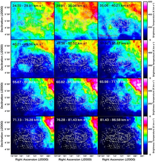
Channel map of H i line emission observed with the GALFA-H i survey. The velocity range is from 24.75 to 86.58 km s−1 with a velocity bin of 5.15 km s−1. The angular resolution is 4′. The gray contours show the total intensity between 1.440 and 1.490 GHz observed with the VLA in 2017. The magenta box in the top-left panel indicates the region referred to in figure 4.
Both panels of figure 7 are position–velocity diagrams. The dashed magenta box in the upper-left panel of figure 6 shows the integrated area of these position–velocity diagrams. A cavity-like structure appears in both diagrams centered on the velocity 44 km s−1 with a range between 33 and 55 km s−1. These trends correspond to the cavity surrounding W 50 shown in figure 6. A similar structure is seen in SNRs (Sano et al. 2017, 2019). An SNR sweeps up surrounding H i clouds, and a cavity appears in an intensity map and a position–velocity diagram. Cavity structures can also be observed around AGNs as a result of interaction between outflows and the surrounding medium (Panagoulia et al. 2014). This means that W 50 can form a cavity regardless of the origin of the spherical shell of W 50, whether an SNR or jets from SS 433. Therefore, the H i cavity is evidence of the interaction between W 50 and the interstellar medium. Assuming the velocity field of our galaxy, we can derive the distance of W 50 using the velocity information of the related H i gas (Brand & Blitz 1993). The distance of W 50 is estimated as 3.0 kpc using the center velocity of the cavity, 44 km s−1. As mentioned in section 1, this distance is different from values obtained with other methods. The distance of W 50 is still under discussion, and it is difficult to conclude from our analysis. We mention the distance of the SS 433/W 50 system again in subsection 4.2.
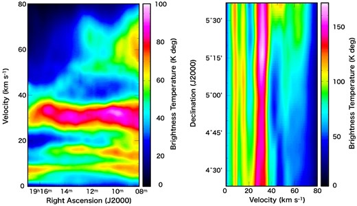
Position–velocity diagrams around W 50. The integrated region is shown in figure 6. The left panel is the velocity distribution in the direction of right ascension. The right panel is a similar map for the direction of declination.
4 Discussion
In this section, we estimate the velocity of the ETF (Filament 5 in figure 11 in the Appendix). We also construct a jet model and discuss the deceleration of the jet. Using the velocity estimate, we derive the maximum energy of cosmic-ray particles accelerated at the jet terminal. Finally, we consider the GeV gamma-ray emission scenario of interaction with the H i cavity and the total energy of protons accelerated by W 50.
4.1 Velocity of the eastern terminal filament
Goodall, Blundell, and Bell Burnell (2011b) derived the upper-limit velocity of the ETF as 0.0405 c. This means that for a propagation velocity of 0.0405 c, the filament observed in 2017 should shift eastward by 15″ from the position in 1984, assuming a distance of 5.5 kpc. If we assume a distance of 3.0 kpc, the upper-limit velocity becomes 0.0221 c, and the filament also moves about 15″. The expected shift is larger than the astrometric error. We compared the positions of the ETF between 1984 and 2017 as follows.
First, we examined the right ascension offsets between SS 433 and the peak positions of the filament in each observation period. After that, we subtracted the offsets of the 1984 observation from those of the 2017 observation. The result is shown in figure 8. None of the peak positions of the ETF has an offset exceeding the astrometric error of ∼|${8{^{\prime \prime}_{.}}74524}$|. This means that the ETF was stable for 33 yr and did not move with the upper-limit velocity estimated by Goodall, Blundell, and Bell Burnell (2011b).
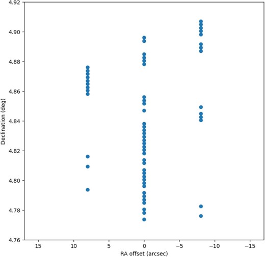
Right ascension offsets of the peak positions along the ETF from SS 433 between 2017 and 1984.
4.2 Comparison between observation and energy conservation jet model
Goodall, Blundell, and Bell Burnell (2011b) suggested that a continuous, non-multi-episodic jet cannot be decelerated below the upper-limit velocity 0.0405 c by interaction with the surrounding ISM. However, Panferov (2017) suggested that the jet could be decelerated by viscosity between the jet and its surroundings. They also estimated that the jet velocity decreases by ∼60% within the spherical shell of W 50, although the value is still higher than the upper-limit velocity estimated in subsection 4.1.
Here, we use a one-dimensional model of the velocity of the terminal of the continuous jet, assuming kinetic energy flux conservation (Zaninetti 2016), with and without the initial spherical shell of W 50. On the basis of the result, we determine whether the continuous jet can be decelerated below the upper-limit velocity at the current position of the eastern jet terminal. We also discuss the formation scenario of W 50 considering the formation timescale and the propagation distance of the western jet.
Figure 9 (left) shows the relation between the velocity of the terminal of the eastern jet and distance from SS 433 in Model A, equations (10) and (11), assuming a distance of 5.5 kpc for SS 433. In this case, the shell radius is |x1| = 48 pc and the terminal of the eastern jet propagates about x = xt = 100 pc, where xt is the distance of the eastern terminal from SS 433. At position xt, the velocities of the terminal decrease to 0.0016 c (480 km s−1), 0.00073 c (219 km s−1), and 0.00034 c (102 km s−1) for ζ = 10, 100, and 1000, respectively. These values are all below the estimated upper-limit velocity of 0.023 c (6895 km s−1). If we assume a distance of 3.0 kpc for SS 433, |x1| = 26 pc, and x = xt = 55 pc, the velocities of the terminal region are 0.0012 c (360 km s−1), 0.00057 c (171 km s−1), and 0.00026 c (77.9 km s−1) for ζ = 10, 100, and 1000, respectively. These results seem consistent with the observation. Figure 9 (right) shows the relation between the time and distance from SS 433. The solid and dashed lines correspond to the eastern and western jets, respectively. Because the distance of the terminal of the eastern jet is about xt = 100 pc from SS 433, it takes 133140 yr, 257192 yr, and 524454 yr to reach the current position for ζ = 10, 100, and 1000, respectively. These times are too long to maintain the continued jet. In addition, the western terminal propagates about 69 pc in all cases assuming a distance of 5.5 kpc, which is larger than the observed value of 56 pc by about 23%. Thus, it is difficult to explain the formation of W 50 with Model A.
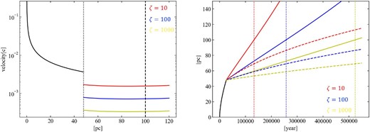
(Left) Relation between the distance from SS 433 and velocity of the eastern terminal in Model A. The distance of SS 433 is assumed to be 5.5 kpc. The black solid line shows the relation within the spherical shell, whose radius is marked with a black dotted line (|x1| = 48 pc). The red, blue, and yellow solid lines correspond to the relation outside the shell for ζ = 10, 100, and 1000, respectively. The black dashed line shows the recent position of the eastern terminal of the jet (xt = 100 pc). (Right) Relation between the time and distance of the eastern and western terminals in Model A. The solid and dashed lines correspond to the eastern and western terminals, respectively. The dotted lines show the time when the eastern terminal region reaches the current position.
Figure 10 shows the corresponding results for Model B, equation (13). When the eastern jet propagates to the distance xt = 100 pc, the terminal velocity is 0.0049 c (1469 km s−1), and it takes 54660 yr to reach the current position. At that time, the terminal of the western jet propagates about 62 pc. Considering the propagation time scale and the distance ratio between the eastern and western wings, Model B is slightly better than Model A for a distance of 5.5 kpc. The 10% difference in the propagation scale of the western terminal between Model B and observation is still larger than the astrometric error. This could be explained by the local distribution of the surrounding ISM. Although we cannot conclude that Model B is more appropriate than Model A, the result implies that the SS 433 jets might be able to construct the morphology of W 50 without an initial wind-bubble shell or SNR, as suggested by Ohmura et al. (2021).
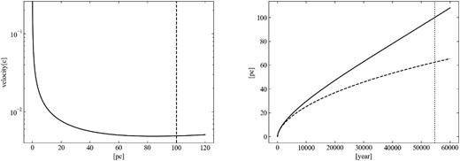
Similar to figure 9, but for Model B.
However, if we assume the distance of SS 433 to be 3.0 kpc with Model B, the eastern terminal velocity is 0.0032 c (959 km s−1), and it takes 39392 yr to reach the current position. At that time, the western terminal region propagates about 41 pc in this model. This is longer than the observed value of 31 pc. This result might imply that the distance of 3.0 kpc derived from the velocity of the H i cavity surrounding W 50 is doubtful; however, we suggest that the H i cavity is still correlated with W 50. Observational and numerical studies have revealed that the peculiar motions of gases, stars, and star-forming regions induced by localized turbulence could yield systematic errors in kinematic distances of a few kpc (see Baba et al. 2009; Ramón-Fox & Bonnell 2018, and references therein). Then, the central velocity of the H i cavity may reflect the influence of the peculiar motion of H i gas interacting with the SS 433/W 50 system.
4.3 Maximum energy of accelerated protons at the jet terminal region
Our estimation implies that the SS 433 jet can accelerate cosmic-ray particles above the energy of 1015.5 eV, although we need to investigate the appropriate value of ηB by additional observations. This result is consistent with recent theoretical and numerical studies (Cooper et al. 2020). Future high-sensitivity gamma-ray observation by the CTA might detect emission induced by the interaction between cosmic-ray protons and the surrounding ISM protons.
4.4 Total energy of accelerated protons
Recently, GeV and TeV gamma-rays have been detected around W 50 (Bordas et al. 2015; Abeysekara et al. 2018; Sun et al. 2019; Li et al. 2020; Fang et al. 2020). As mentioned in section 1, although Sun et al. (2019), Li et al. (2020), and Fang Charles, and Blandford (2020) used almost the same Fermi-LAT dataset, they suggested different positions and processes for the GeV gamma-ray excess. Wherever gamma-ray emission is induced, cosmic-ray protons should interact with the surrounding ISM protons in the hadronic scenario. Moreover, the H i cavity mentioned in subsection 3.2 is most likely the origin of the gamma-ray emission. In this section, we estimate the total energy of cosmic-ray protons accelerated by the SS 433/W 50 system in the hadronic scenario without strictly considering the accelerating position, i.e., whether it is the spherical shell or the SS 433 jet.
5 Conclusions
In this paper, we provided a new continuum image of W 50 in the L band. We compared the result with the observations in 1984 and 1996 and found that W 50 did not experience any shape change for 33 yr. There are many H i clouds around W 50 within a broad velocity range. We focused on the clouds in the velocity range from 33.77 to 55.85 km s−1 because of the cavity structure, which seems to coincide well with the shape of W 50. We estimated the upper-limit velocity of the ETF at 0.013 c and 0.023 c, assuming distances of 3.0 and 5.5 kpc. We considered two energy-conservation jet models, with and without the initial spherical shell, and the observationally estimated upper-limit velocities satisfy the presumed velocity based on these jet models. Furthermore, our analysis implies that the non-initial-spherical-shell scenario assuming a distance of 5.5 kpc better explains the formation of W 50, although we cannot still reject the initial-spherical-shell scenario. Using the estimated upper-limit velocity, we predicted the maximum energy of cosmic-ray particles accelerated by the jet terminal above the energy of 1015.5 eV. Finally, we estimated the total energy of the accelerated cosmic-ray protons using the luminosity of the GeV gamma-ray emission. We assumed the H i cavity was interacting with W 50 and estimated its density in both optically thin and thick H i gases. The estimated energies are in the range 6.2 × 1047–5.2 × 1048 erg, depending on the density of the H i cavity and the distance of W 50. These values are lower than for typical middle-aged SNRs, which implies that the GeV gamma-ray emission originates in the SS 433 jet.
Acknowledgements
We are grateful to Drs. K. Tachihara, H. Yamamoto, H. Sano, R. A. Perley, T. Tsutsumi, A. J. Mioduszewski, and V. Dhawan for useful discussion. This work was supported by JSPS KAKENHI Grant Numbers HS: 20J13339, TO: 20J12591, and MM: 19K03916 20H01941. Data analysis was partly carried out on the Multi-wavelength Data Analysis System operated by the Astronomy Data Center (ADC) at the National Astronomical Observatory of Japan. This work was supported by the Japan Foundation for Promotion of Astronomy. The National Radio Astronomy Observatory is a facility of the National Science Foundation (NSF) operated under a cooperative agreement by Associated Universities, Inc. This publication uses data from the Galactic ALFA H i (GALFA H i) survey conducted with the Arecibo L-band Feed Array (ALFA) on the Arecibo 305 m telescope. The Arecibo Observatory is operated by SRI International under a cooperative agreement with the National Science Foundation (AST-1100968), and in alliance with Ana G. Méndez-Universidad Metropolitana and the Universities Space Research Association. The GALFA H i surveys were funded by the NSF through grants to Columbia University, the University of Wisconsin, and the University of California. SAOImageDS9 development was made possible by funding from the Chandra X-ray Science Center (CXC), the High Energy Astrophysics Science Archive Center (HEASARC), and the JWST Mission office at the Space Telescope Science Institute (Joye & Mandel 2003). This research used Astropy 〈http://www.astropy.org〉, a community-developed core Python package for astronomy (Astropy Collaboration 2013, 2018). Mark Kurban from Edanz Group 〈https://en-author-services.edanz.com/ac〉 edited a draft of this manuscript.
Appendix. Summary of the radio continuum image in 2017
Figure 11 shows a total intensity image of W 50 observed in 2017. For clarity, we name characteristic structures and indicate them with arrows. The frequency coverage is from 1.340 to 1.902 GHz, except for frequencies between 1.507 and 1.726 GHz. Although there are artifacts around W 50, they have less influence on image quality. There is also a negative bowl northwest of W 50 due to a lack of the shortest UV-spacings.
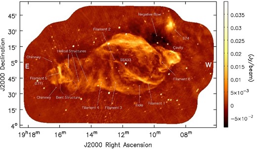
Total intensity map of SS 433/W 50. The frequency coverage is from 1.340 to 1.902 GHz. Note that the frequencies between 1.507 and 1.726 GHz are excluded owing to radio frequency interference. This image consists of 58 pointings. The ellipse at the bottom-left corner shows the beam size of 53″ × 43″. The rms noise level is 0.49 mJy beam−1. Beside SS 433/W 50, there are many sources in this field of view, including bright extragalactic sources and the H ii region S74 in the northwest. “E” and “W” indicate the east and west directions, respectively.
We succeeded in resolving many characteristic structures of W 50. The bright filament near SS 433 is resolved and curves southwest (Filament 1). Filament 1 seems to be branched near SS 433. Below Filament 1, there is a dark hole identified by the Low Frequency Array (LOFAR) observation at 150 MHz (Broderick et al. 2018). Another faint filament is northeast of SS 433 (Filament 2). It spatially coincides with the predicted rim of the helical jet, which has an opening angle of about 20° (Margon 1984). The northern region of the central shell is especially bright and extends in the east–west direction. Some filaments seem to overlap in this region. The bright region has been suggested as resulting from interaction between the spherical shell and surrounding ISM. Because the southern shell is far from the Galactic disk, it is dimmer than the northern shell. Finally, two diffuse filaments extend from the southeast rim of the shell towards the north direction (Filaments 3 and 4). Filament 3 (the longer one) seems to consist of two overlapping filaments.
The eastern wing has a uniquely undulated shape and has several characteristic structures. The most noticeable one is a bright filament extending along the north–south direction at the eastern edge (Filament 5). We call Filament 5 the eastern terminal filament (ETF). The bright part extends to the north; however, the southern region becomes dimmer and branches off. Previous studies have resolved a faint structure called a “chimney” extending to the northeast region of the ETF (Dubner et al. 1998; Farnes et al. 2017; Broderick et al. 2018). Although it is very faint, we can find the chimney in a region about 7′ in size. The difference from previous observations (Farnes et al. 2017; Broderick et al. 2018) is that the southern chimney is clearly identified. There is a bent structure on the western side of the southern chimney, and the diameter of the eastern wing seems to change at this point. We also find unique helical structures that coil around the eastern wing. While the helical structures are similar to Filaments 3 and 4, they differ in the curve direction.
The western wing is shorter than the eastern one because the western side of W 50 is near the Galactic disk, and the jet interacts with a denser medium. There is a faint filament perpendicular to the jet axis (Filament 6) at the base of the wing. The boundary area of the western wing seems very bright; however, the inner region is a cavity. A molecular cloud is located at the cavity, and Liu et al. (2020) suggested that the molecular cloud detected by Yamamoto et al. (2008) is in the western wing.
The background emission of the western area has an uneven structure owing to the Galactic disk. The H ii region S74 can be seen clearly in the northwest direction from W 50. There are many point sources in the entire image, which are believed to be extragalactic sources except for SS 433.
Footnotes
ngVLA Memo Series No. 17, 〈http://library.nrao.edu/ngvla.shtml〉.
