


Abstract
We have developed a new method for detecting near-Earth objects (NEOs) based on a Field Programmable Gate-Array (FPGA). Unlike conventional methods, our technique uses 30–40 frames to detect faint NEOs that are almost invisible on a single frame. To reduce analysis time, image binarization and an FPGA-implemented algorithm were used. This method has aided in the discovery of 11 NEOs by analyzing frames captured with 20 cm class telescopes. This new method will contribute to discovering new NEOs that approach the Earth closely.
1 Introduction
Near-Earth objects (NEOs) are a global threat. The well-known Tunguska meteor was an NEO a few dozen meters across. It struck Siberia in 1908 (Chyba et al. 1993), and incinerated the forest for 30–50 km around. The Chelyabinsk meteor was a 20 m NEO that damaged more than 7300 buildings and injured 1500 people. NEOs of this size range cause such severe local damage that discovering them early in their approach is a top priority.
The distribution of small main belt asteroid (MBA) bodies larger than 300 meters is known (Yoshida et al. 2003; Yoshida & Nakamura 2007; Mainzer et al. 2011), but the distribution of a few dozen meters MBAs remains unclear. Determining the distribution of their size would help us to understand how to move the original materials throughout the solar system and when organic substances which became the origin of life were created. NEOs have an increasing chance of being detected as they approach the Earth. However, the many NEO survey groups miss most NEOs of this small size.1–3
Large-format optical cameras like the Hyper Suprime-Cam (Miyazaki et al. 2018) and Tomo-e Gozen (Sako et al. 2016) have provided a huge amount of sky data. Processing the large data sets needs high-speed analyses. Using an FPGA (Field Programmable Gate-Array) and/or a GPU (Graphics Processing Unit) is two solutions. Our new method employs a new NEO detection algorithm that utilizes an FPGA.
Most NEO survey groups use the conventional blink method to detect NEOs (Copândean et al. 2018). In the blink method, moving objects are searched using several frames in which they are visible. Our method uses 30–40 frames to detect faint NEOs that are almost invisible on a single frame.
Our method is far more computationally intensive than the blink method, but image binarization and implementing the algorithm on an FPGA board increases the speed in analysis dramatically. We detected 11 NEOs of a few dozen meters across using 20 cm class telescopes by our method. This means the method will help us to discover NEOs of the undiscovered size range using very small telescopes. Section 2 describes the algorithm in detail, while sections 3 and 4 explain the analysis procedure and the NEO survey observation using the method, respectively.
2 New NEO detection method
2.1 The basic algorithm
We developed an algorithm that enables us to detect faint moving objects in the sky automatically (Yanagisawa et al. 2005). The algorithm has three parts: (1) preparing multiple frames of the same field of view; (2) cropping each frame to follow the track of a possible NEO (indicated by a shifted value of image pixels); and (3) combining the cropped frames through a median filter. This sequence is repeated for the various shifted values. Processing a cropped frame with a median filter enhances its signal-to-noise ratio significantly and reduces the incidence of high-value noise events such as hot pixels and cosmic-ray strikes. A similar process was developed by Shao et al. (2014), but they used the sum filtering instead of the median filter processing. Figures 1 and 2 summarize the algorithm and show an example of asteroid detection. Figure 2a is a raw frame and figure 2b is the final image, processed by the algorithm over 40 frames. The object in figure 2b is an asteroid moving within the frames; it must be within the circle of figure 2a. Figure 2 shows the great advantage of the algorithm.
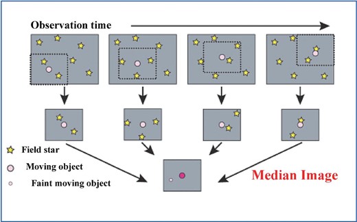
Automatic detection original algorithm. (Color online)
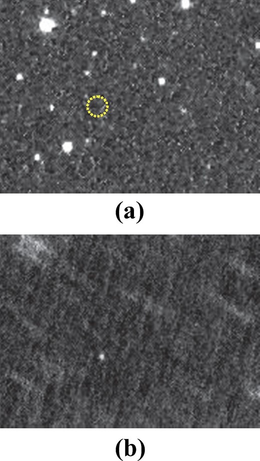
Apparition of an asteroid detected by the original algorithm. (Color online)
2.2 Implementing the new algorithm in an FPGA
Although the algorithm described above is useful for detecting faint objects well, the median filtering of dozens of frames and the calculation for various motions take enormous time. For example, a conventional PC takes about 280 hr to calculate 65536 motions for 32 1 K × 1 K frames involving a search for objects by the motion of 256 × 256 pixels in 32 frames. Since capturing 32 images takes only 15 min in our NEO survey observations, the 280 hr that the algorithm takes is not practical.
The solution is creating binarized images using a proper threshold and then calculating the sum of the binarized images. This gives almost the same result as the basic algorithm, but it reduces the analysis time to almost one percent (Yanagisawa & Kurosaki 2014).
Figure 3 shows the difference between the images generated by the original algorithm and by the new one. The upper panels show the original image sequence, and the lower panels show the new image one. The white regions in the lower panels have values higher than one proper threshold (the first threshold), while the black ones have lower values. The assignment of values 1 and 0 to the white and black regions, respectively, is called image binarization. The right-hand lower panel is the final image produced by the new algorithm. The image is created by summing the binarized frames created using the first threshold following the track of a moving object, and by binarizing the resulting frame using a second threshold. The first threshold is set according to the faintness of the detected object. If a low threshold is set, most of the white regions are back-ground noise or field stars. The second threshold is set based on how many frames contain the object of interest; a high second threshold indicates that the object is likely to be real and not an accidentally well matched noise.
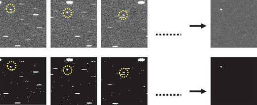
Comparison between detections by the original algorithm using median (upper panels) and the modified one using binarization (lower panels). (Color online)
Therefore, the selection of the first and second thresholds is very important in detecting faint objects; in particular, setting a wrong threshold value can generate a lot of noise detections or detections of only bright objects. The correct threshold values are determined by checking the number of false detections by analyzing randomly shuffled frames according to the observation time given for an instrument and telescope.
Figure 4 shows the number of false detections for various first and second threshold values in the case of 65536 calculations for 32 1 K × 1 K frames. The x-axis is the second threshold value, each line represents a first threshold value, and the y-axis is the number of false detections. As one can see, setting lower values for the first- and second-threshold values results in many false detections. The new algorithm is so simple that we can implement it in an FPGA board. Figure 5 shows the FPGA board, an Expresso A5, manufactured by Soliton Systems. The board can calculate 65536 processes of 32 2 K × 2 K)not 1 K × 1 K(within 40 s, which enables us to analyze real-time NEO observation data (32 2 K × 2 K frames taken every 15 min). The more frames are used, the fainter objects can be while still being detectable. However, many computational resources are required for analyzing many frames. Thirty–forty frames are adequate, considering the current FPGA and PC performances used in our system.
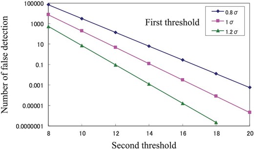
Number of false detections for various first and second thresholds. The x-axis is the second threshold, each line represents a first threshold, and the y-axis is the number of false detections. (Color online)
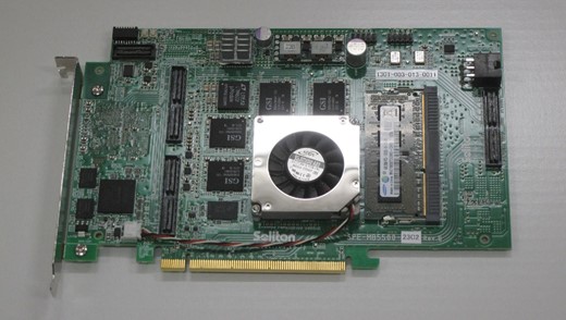
FPGA board, Expresso A5, manufactured by Soliton Systems.co., LTD. (Color online)
The possible apparent velocities (proper motion) of the expected moving objects depend on the pixel sizes of the sensors and the exposure time for one frame. To be detected with the algorithm, the objects must move more than 3 pixels during the 15 min interval. Considering the typical pixel size of |$6.\!^{{\rm{^{\prime\prime}}}}2$| per pixel and the typical exposure time of 24 s for our observation equipment, the minimum apparent velocity is |$1.\!^{{\rm{^{\prime\prime}}}}26$| per min. Although objects that are faster than this are detectable, the detection ability decreases after the motion of the objects during the exposure time exceeds the pixel size, which is |$13.\!^{{\rm{^{\prime\prime}}}}2$| per min. The optimum exposure time should be set considering the velocity range of the targeted moving objects (MBAs, NEOs, space objects in the geostationary orbit, or those in the low Earth orbit).
2.3 Modification of the new algorithm
We discovered two NEOs (2017 BK and 2017 BN92) using the algorithm described in subsection 2.2 (Yanagisawa et al. 2017). The apparent magnitudes of these NEOs are 17.5 (2017 BK) and 17.1 (2017 BN92) in the V band, respectively. Observations were made at JAXA’s Mt. Nyukasa Observational Facility in Nagano, Japan. The equipment included two 18 cm telescopes (from Takahashi; an ϵ180ED), a commercial CCD camera (from FLI, an ML23042), and a CMOS camera (from Canon, Inc.) for a 1000 deg2 survey over four nights. The pixel sizes for the two sensors are |$6.\!^{{\rm{^{\prime\prime}}}}2$| per pixel (ML23042) and |$7.\!^{{\rm{^{\prime\prime}}}}8$| per pixel, respectively. The typical seeing value at the facility is about |$3.\!^{{\rm{^{\prime\prime}}}}5$|. Discovering NEOs using very small telescopes and the algorithm like this represents a novel method. The NEOs had absolute magnitudes of 24.0 and 25.6 (about 70 m and 30 m in size, assuming an albedo of 0.1.), which are quite faint and difficult to find even with current big surveys. The effectiveness of the algorithm contributed to these discoveries and we proved that the algorithm is a powerful tool in finding NEOs that come very close to the Earth.
However, the algorithm can be further improved. As figure 4 shows, lowering the first threshold leads to excessive false detections that are caused by the many pixels with a value of 1. Using the threshold for image binarization causes many invalid value-1 areas (flares) around bright field stars and moving objects. This makes it necessary to use higher thresholds to detect real objects. This problem can be partially solved by defining an object candidate. The object candidate pixel(s) must have a higher value than the set threshold value, and must be higher than those of the surrounding eight pixels. Figure 6 shows how the object candidates work. Figure 6a is a part of the original image. Figures 6b and 6c show the binarized images using a threshold and the object candidate, respectively. As one can see, the value-1 areas of the binarized image using the object candidate are much smaller than that using a threshold. This enables the algorithm to lower the threshold.
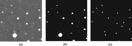
Difference of the two image binarizations. (a) Original image. (b), (c) Binarized images using a threshold and the object candidate, respectively.
As observed frames are cut off on a pixel basis to follow the presumed motion, one pixel for the object candidate may not match exactly to the same coordinate of the cut-off frames in the algorithm. To cope with the situation, three neighboring pixels that show the maximum total value among four cases described in figure 7, are selected. The left-hand image in figure 7 shows the pixel values around the pixel of the object candidate. The middle panel shows the top view of the left-hand image. The value of each 2 × 2 set (shown in dotted lines) is calculated. The four pixels with the maximum total value (the image on the right) are set to 1. The moving object has a high probability of residing in the 4 pixels. The 3 pixels instead of the surrounding 8 pixels are used to reduce the value-1 areas in the frames. Figure 6c shows the result of the modification—less flare and an improved chance of detecting objects of fainter magnitude. The number of object candidates is adjusted to detect real objects. The number is defined in the same way that the first threshold is determined in subsection 2.2. This modification improves the detection sensitivity by 1.0 mag.

Three pixels selection process. Left: The pixel values around the pixel of the object candidate. Middle: The top view of the left-hand image. The sum value of each 2 × 2 set (shown in dotted lines) is calculated. The four pixels with the maximum total value (the right-most image) are set to 1. (Color online)
3 The analysis processes of the NEO detections
Figure 8 is a detailed flow chart of the NEO detection process. The system continues taking 32 2 K × 2 K-frames of 24 s exposures during 15 min intervals. Six 20 cm class telescopes equipped with the large optical sensors change their observing areas every 15 min to survey a large region of the sky. The details of this system are described in section 4.
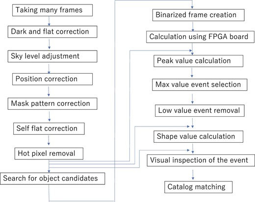
Flow chart of the NEO detection process. (Color online)
After dark-frame subtraction and flat-fielding, the sky level adjustment is made. First, the sky level of each frame is calculated using the sigma clipping technique. Then, all 32 frames are adjusted (leveled) to the median of the 32 sky levels.
The position correction removes small shifts in the field of view caused by sidereal tracking error. The brightest pixel of one field star around the central region of the first frame is selected as its marker. The maximum valued pixel in the next frame around the small region (|$11\,\, \times 11\,\,{\rm{pixels}})$| near the pixel of the first frame is searched for, and this process is repeated through the last frame. The shift-removed common regions are created using the pixel coordinates on each frame.
The mask pattern correction is one of the most important processes and is adapted from Yanagisawa's paper (Yanagisawa et al. 2005). Figure 4 in their paper gives an overview of the process. The mask pattern correction can remove most of the field-star features and sky-level gradient caused by insufficient flat-fielding or observation of low elevations.
As we search the object candidates, the flatness of the frames is very important. The flat-fielding and mask pattern correction do not suffice since the sky level pattern sometimes changes by the second with atmospheric turbulence. The self-flat image is created by sigma clipping and smoothing each mask pattern corrected frame. By dividing the mask pattern corrected frame with the self-flat image, a perfectly flat frame is obtained.
Hot pixels with higher values than the surrounding pixels are replaced with the median value of the surrounding eight pixels. The frames after the hot pixel removal are used for the processing in the search for object candidates, peak value calculations, shape value calculation, and visual inspection of the event.
As described in subsection 2.3, the object candidates are searched in the 32 frames after the hot pixel removal. If the threshold is low, the number of candidates is high. In order to avoid false detections, the threshold is adjusted to pick 160000 candidates in each frame. In this process, the three pixels described in subsection 2.3 and shown in figure 7 are also selected.
Setting the value to 1 for the object candidates and the neighboring three pixels and setting the value to 0 for the other pixels creates 32 binarized frames. These binarized frames are input to the FPGA board, which consists of the Intel Arria V GZ FPGA chip and four banks of DDR3 SDRAM.
The FPGA board calculates the sum of the 32 binarized frames considering the shifted values described in the subsection 2.1 for dx and dy from |$- 255$| to 255 pixels, respectively. There are a total of 261121 calculations, which are required to be completed by the FPGA board within 160 s. The second threshold described in subsection 2.2 is set to 21 in our case. The FPGA board returns the coordinates of x and y, and the shifted values of dx and dy that satisfy the threshold condition.
Moving objects usually satisfy the threshold condition at various combinations of the coordinates and the shift values that are close to each other as the objects spread to a few pixels. To find their true values, the peak value is investigated by creating the median of 32 small portions of the hot-pixel-removal frames that match the combination of the coordinates and the shifted value. In the group of the combinations showing close values of the coordinates and the shifted values, the combination that has the maximum peak value is considered a true event.
The combinations that have a lower peak value than the threshold are considered as noise and removed.
The shape value is defined as the sum of the values of the |$3\,\, \times 3\,\,{\rm{pixel\,\,}}$| group divided by the central value. The values are checked for all combinations after low-value event removal by calculating the median of the 32 small portions of the hot-pixel-removal frames. A shape value close to 1 indicates that the central pixel is extremely high and may be noise.
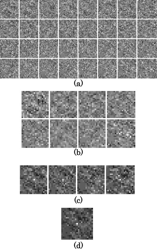
The observer checks the result file containing the shifted values (dx, dy) representing total motion in pixel during the 15-min interval, the coordinates (x, y) representing the position in pixel at the first image, the peak value, and the shape value as described in table 1. Although an observer can tell which objects are really moving objects based on the peak values (for example, higher than 20.0) and the shape values (for example, higher than 3.0), visual inspections are carried out for the final check using the 32 small portions of the hot-pixel-removal frames that match the combination of the coordinate and the shifted value. Figure 9 shows the images of the real event that was visually inspected. The 32 images in figure 9a represent the individual frames, after shifting the cropped small region in which a nearly invisible NEO is located (in the center of all these images). Figures 9b–9d represent the combined images of the 4, 8, and 32 images with median filer, respectively. One can see the signal of the object increased as the number of the image is increased. Figure 10 shows the case of noise. An observer can easily discriminate a real event from noise by checking these images. In the future, this process will be replaced by a machine-learning algorithm to reduce the burden on the observer.

Visual inspection images of a real event. (a) Thirty-two images of the individual frames, after shifting the cropped small region in which a nearly invisible NEO is located (in the center of all these images). (b), (c), (d) Combined images of the 4, 8, and 32 images with median filer, respectively.
Visual inspection images of a noise event. (a) Thirty-two images of the individual frames, after shifting the small cropped region. (b), (c), (d) Combined images of the 4, 8, and 32 images with median filter, respectively.
Sample of the result file for one field.*
| dx | dy | x | y | Peak | Shape |
|---|---|---|---|---|---|
| –88 | 13 | 971 | 1359 | 64.86 | 4.01 |
| –49 | –83 | 169 | 414 | 25.92 | 4.29 |
| –188 | –106 | 327 | 536 | 19.32 | 1.67 |
| –103 | 11 | 1972 | 1851 | 17.27 | 1.82 |
| –5 | –30 | 1985 | 157 | 15.96 | 2.97 |
| –47 | 101 | 1770 | 1579 | 15.78 | 3.32 |
| –25 | –35 | 1200 | 510 | 15.39 | 1.46 |
| 138 | –74 | 212 | 891 | 15.01 | 1.92 |
| … | … | … | … | … | … |
The result file contains the shifted values (dx, dy) representing total motion in pixel during the 15 min interval, the coordinates (x, y) representing the position in pixels at the first image, the peak values, and the shape values of the event candidates.
Finally, catalogue matching is done by comparing the Hubble guide star catalogue ACT with the coordinates of background stars to extract the celestial coordinates of the moving objects. By using the shifted values (dx, dy) and the coordinates (x, y) of the moving objects described in the result files (like table 1), the celestial coordinates on the first and last images are extracted. These two celestial coordinates are used for reporting the discovery of NEOs to the Minor Planet Center.4 The codes for all these processes are written in C++.
4 NEO survey at Australia's Siding Spring Observatory
Besides the Mt. Nyukasa Observational Facility, JAXA operates a remote observation site at Siding Spring Observatory in Australia. Figure 11 shows the three equatorial mounts that are set in a sliding roof. The first mount is a fork-type equatorial mount (from Mathis Instruments, an MI-500) that holds four 18 cm telescopes (from Takahashi, ϵ180ED); there are two CMOS sensors (from Bitran, BH-60M-KAI), a CMOS sensor (from FLI, a KL4040), and a CCD camera (also from FLI, a ML23042) mounted on the four telescopes. The second and the third mounts are both fork-type equatorial mounts (from Celestron, CPC800DX). A 25 cm telescope (from Tanaka Koukagaku Kougyou, a K.K.BSC250C-II) and an 18 cm telescope (from Takahashi, an ϵ180ED) are installed on the two mounts, and two CCD cameras (from FLI, ML4240 and ML23042) are attached to these two telescopes. The typical pixel size is |$6.\!^{{\rm{^{\prime\prime}}}}2$| per pixel and the typical seeing value at the site is about |$2.\!^{{\rm{^{\prime\prime}}}}5$|.
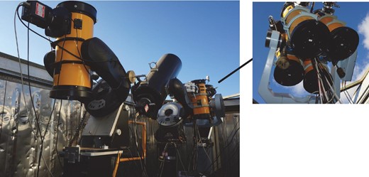
JAXA’s remote observation site at Siding Spring Observatory in Australia. Left: Three equatorial mounts. Right: The first mount (seen on the furthest right in the left-hand panel) holding four 18 cm telescopes. (Color online)
We have run the NEO survey there using the algorithm and processes described in sections 2 and 3 since 2018 January. Six telescopes observed different sky regions every 15 min covering 2764 deg2 per night. One night's data is about 52 GB. An observer programs each pairing of a telescope and a camera remotely at the beginning of the night. All the data from the six sensors are stored at the NAS system and analysed automatically by an FPGA machine, which contains the two FPGA boards described in section 3, and a 40-core PC, (a HPC5000-XBW216TS-Silent) that performs other duties than FPGA processing. The observer only checks the result files (see table 1) after the shape value calculations. After the visual inspection of an event, catalogue matching is done to extract the two celestial coordinates of the event. These coordinates are used for checking if the event is a known object according to the Minor Planet Center website. If the event is an unknown object, this may be a new NEO. The observer then stops the survey operation of the second or third mount and points its telescope at the event, and follows up the event assuming the event has a uniform linear motion. The processes of the follow-up observation and data analysis are the same as those for the survey observation. After extracting the two celestial coordinates of the event from the follow-up observation data, all four celestial coordinates (including the two extracted in the survey observation) are reported to the Minor Planet Center by email. The details of the reported event will be given on the Center's website, including the temporal orbital elements and the ephemerides, so that other observers can follow up the event to determine the precise orbit of the object. The equatorial mount goes back to making the survey observations when it finishes the follow-up.
We have discovered nine NEOs in Australia so far, covering a total of about 140000 deg2, observed during about 50 nights of new moon seasons. Table 2 and figure 12 show the details of 11 NEOs discovered using the method and their current positions. As shown in table 2, the method can detect 10 m NEOs, which are quite difficult to discover using current NEO survey programs such as Pan-Starrs, CSS, and Atlas. All the NEOs were discovered close to the Earth, which means that their apparent velocities were very high, as shown in table 2. These NEOs might have been missed by conventional NEO survey programs. Expanding the observational and data analysis systems of the method would be relatively easy and more cost-effective than establishing a conventional NEO survey program using a large telescope and a large sensor.
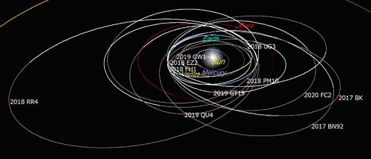
Current positions of the 11 NEOs discovered by the method. (Color online)
Details of the 11 NEOs discovered using the method.
| ID | Discovery date | Brightness (V) | Velocity (arcmin d-1) | Family | e | a (au) | i (°) | RAAN (°) | Absolute magnitude | Size (m) |
|---|---|---|---|---|---|---|---|---|---|---|
| 2017 BK | 2017.1.17 | 17.5 | 315 | Apollo | 0.489 | 1.909 | 6.6359 | 110.89 | 24 | 67 |
| 2017 BN92 | 2017.1.31 | 17.1 | 621 | Apollo | 0.483 | 1.921 | 1.0734 | 324.06 | 25.6 | 32 |
| 2018 EZ2 | 2018.3.12 | 18.2 | 279 | Apollo | 0.51 | 1.951 | 4.9718 | 173.92 | 26.6 | 20 |
| 2018 FH1 | 2018.3.18 | 18.7 | 733 | Aten | 0.177 | 0.938 | 3.5468 | 181.41 | 26.6 | 20 |
| 2018 PM10 | 2018.8.9 | 18.3 | 1285 | Amor | 0.427 | 1.78 | 9.2065 | 317.51 | 27 | 17 |
| 2018 RR4 | 2018.9.11 | 18 | 1418 | Apollo | 0.621 | 2.637 | 3.1793 | 351.37 | 27.1 | 16 |
| 2018 UG3 | 2018.10.31 | 19.4 | 510 | Apollo | 0.423 | 1.662 | 6.1673 | 47.27 | 24.5 | 53 |
| 2019 GW1 | 2019.4.4 | 17.5 | 1638 | Aten | 0.114 | 0.934 | 13.2945 | 194.67 | 26.1 | 25 |
| 2019 GT19 | 2019.4.12 | 18.2 | 1018 | Apollo | 0.37 | 1.273 | 7.7488 | 202.69 | 27.5 | 13 |
| 2019 QU4 | 2019.8.28 | 18.1 | 688 | Apollo | 0.332 | 1.426 | 10.1313 | 333.97 | 24.8 | 46 |
| 2020 FC2 | 2020.3.17 | 18.5 | 1870 | Apollo | 0.398 | 1.644 | 6.8153 | 357.15 | 28 | 11 |
5 Conclusions
We developed a new NEO detection method using an FPGA board. The system uses 30 to 40 frames to detect faint moving objects that are invisible on a single frame and enables us to detect NEOs that come close to the Earth with very small telescopes. Using the data taken by 20 cm class telescopes and analysing the data with the method, 11 NEOs were discovered. The telescopes, the sensors, the FPGA board, and the PC used in this work are all commercial-grade equipment, making the system relatively easy and cost-effective to implement. This will contribute to expanding the scale of NEO survey program to find NEOs that are a few dozen meters across.
Footnotes
Acknowledgements
A part of this work was supported by the Innovative Science and Technology Initiative for Security (Grant Number JPJ004596), Acquisition, Technology and Logistics Agency (ATLA), Japan and KAKENHI (16K05546).
