


Abstract
X-ray emission generated through solar-wind charge exchange (SWCX) is known to contaminate X-ray observation data, the amount of which is often significant or even dominant, particularly in the soft X-ray band, when the main target consists of comparatively weak diffuse sources, depending on the space weather during the observation. In particular, SWCX events caused by interplanetary coronal mass ejections (ICMEs) tend to be spectrally rich and to provide critical information about the metal abundance in the ICME plasma. We analyzed the SN1006 background data observed with Suzaku on 2005 September 11 shortly after an X6-class solar flare, signatures of which were separately detected together with an associated ICME. We found that the data include emission lines from a variety of highly ionized ions generated through SWCX. The relative abundances of the detected ions were found to be consistent with those in past ICME-driven SWCX events. Thus, we conclude that this event was ICME driven. In addition, we detected a sulfur xvi line for the first time as one from an SWCX emission, which suggests that it is the most spectrally rich SWCX event ever observed. We suggest that observations of ICME-driven SWCX events can provide a unique probe to study the population of highly ionized ions in the plasma, which is difficult to measure in currently available in situ observations.
1 Introduction
Coronal mass ejections (CMEs) are the most energetic eruptive phenomena in our solar system. The occurrence rate of CMEs depends on the solar activity. Notably, there is a linear correlation between the occurrence rate and sunspot number (Webb & Howard 1994). A CME transfers a large amount of plasma (typically 1015–1016 g) from the low corona to the solar system (Colaninno & Vourlidas 2009). CMEs directed toward the Earth are called “halo CMEs,” named after their coronagraph images. The ejected plasma of a halo CME tends to hit the Earth and is often observed as a disturbance of the solar wind (interplanetary CME, called ICME). While a variety of properties of CMEs and ICMEs have been identified (reviewed, e.g., by Chen 2011; Webb & Howard 2012), the precise mechanisms of their initiation and energy-release procedure are not fully understood.
Since the first detection of a CME in 1971 (Tousey 1973), thousands of CMEs have been detected, mainly in coronagraph observations. In addition to imaging observations, including coronagraph ones, recently developed ultraviolet spectrometers have enabled us to see new characteristics of CMEs, providing essential diagnostic information about the plasma components. Alternatively, information on ICMEs can be obtained in situ by spacecraft. The arrival of an ICME appears as various forms of observable signatures (see the review by Zurbuchen & Richardson 2006). In some cases, ICMEs have enhanced magnetic structures (termed “magnetic cloud” in Burlaga et al. 1981). These magnetic clouds have low proton temperatures and plasma beta (the ratio of the plasma pressure to the magnetic pressure), which are also indicators of the arrival of ICMEs.
ICMEs have also drawn significant attention in X-ray astronomy observations because propagating plasma causes geomagnetic storms, which affect observations with X-ray satellites. In addition to geomagnetic storms, highly ionized ions in the plasma are sources of additional X-rays during observations of celestial objects. These additional X-rays are ascribed to so-called solar wind charge exchange (SWCX), a phenomenon whereby an electron in a neutral atom is transferred to a highly ionized ion in the solar wind during their collisions. When an electron in an excited state falls back to the ground state, the energy is released as one or more photons in the extreme ultraviolet to soft X-ray range. This mechanism was first suggested by Cravens (1997) to explain the line emission spectrum discovered in observations of C/Hyakutake 1996 B2 (Lisse et al. 1996). Freyberg (1998) and Cox (1998) suggested that solar wind could produce X-rays in the exosphere of the Earth (geocoronal SWCX) and in the heliosphere (heliospheric SWCX), and that the mysterious X-ray time variation detected during the ROSAT All-Sky Survey, which was reported by Snowden et al. (1994) and dubbed “long-term enhancement” (LTE), might have originated in the SWCX. Since solar wind, which continually blows into the heliosphere, always interacts to some extent with neutral atoms in the solar system, SWCX is now recognized as a persistent background component in observations of X-ray diffuse sources.
To date, numerous SWCX detections with Chandra, XMM-Newton, and Suzaku have been reported (e.g., Wargelin et al. 2004; Snowden et al. 2004; Fujimoto et al. 2007; for more details see Kuntz 2019). Systematic studies of the time variations of the soft X-ray flux have been conducted with large archival datasets of XMM-Newton and Suzaku (Carter & Sembay 2008; Carter et al. 2011; Ishi et al. 2017). Roughly a hundred observational datasets in each of the XMM-Newton and Suzaku archives have been found to show time variations caused by geocoronal SWCX. This implies that data that contain time-variable SWCX components are not rare, hence the significance of the study of SWCX in order to handle X-ray observational data correctly. While an increasing number of samples of SWCX are now available, it still remains difficult to construct a comprehensive theoretical model that describes the observed properties of SWCX observations, such as time series and overall flux levels, for arbitrary spacecraft look-directions and epochs (Kuntz 2019). One of the major difficulties stems from the fact that the properties of ions in solar wind vary with both solar cycle and solar latitude; the intensity and fluctuation of SWCX emission are highly dependent on the viewing point. However, the global structure of the solar wind, especially at a high solar latitude, cannot be clarified with current in situ measurements. Further X-ray observation in a variety of directions is the only way to refine the entire model, including at high solar latitudes.
In addition to the evaluation of the SWCX model, SWCX events associated with ICMEs also provide us with ionic information on the plasma from various emission lines. The most spectrally rich case of SWCX events reported so far was by Carter, Sembay, and Read (2010), whose systematic study, using the XMM-Newton archive, made unequivocal detections of lines from various ions, including highly ionized neon, magnesium, and silicon. That work is a good precedent that the components of ICME plasma can be identified indirectly with X-ray observations. One of the notable characteristics of the event is that the source ICME was accompanied by an X-class flare. Reinard (2005) suggested a positive correlation between solar flare magnitude and the ionization state of the CME plasma. Providing this correlation is correct, ICMEs associated with large flares should yield spectrally rich SWCX events, which have plenty of information about the ICME plasma. However, the opportunities to detect such spectrally rich events rarely arise because X-class flares are rare in the first place and because not all X-class flares are associated with CMEs. Thus, SWCX events caused by ICMEs associated with X-class flares are valuable samples.
In this paper we report on a newly discovered SWCX emission from the SN1006 background data observed by Suzaku, which is likely to be associated with an ICME accompanied by an X-class flare. This event could not be observed with XMM-Newton, unfortunately, due to the intense solar activity. Conventionally, SWCX emission can be simply identified as a temporal excess from the stable component in the observed X-ray light curve. However, this simple method is not applicable to datasets like the one studied here, where no X-ray time variation is observed within the observation period. Our strategy is to compare the data with other data obtained in the same region at a different observation epoch to subtract the stable component and identify the potential excess. We summarize the observations and our data analysis flow in sections 2 and 3, respectively. Discussion about the correlation with a CME and the significance of this detection is given in section 4.
2 Observations
2.1 SN1006 background
We used the Suzaku data from the region “SN1006 background,” located at (α, δ)J2000.0 = (224|${_{.}^{\circ}}$|65, −42|${_{.}^{\circ}}$|40). The primary purpose of the original observations was to take a dataset to serve as the background for the nearby main target SN1006. This region was observed twice by Suzaku, on 2005 September 11 and 2006 January 26. The average normalized pointing vectors in geocentric solar ecliptic (GSE) coordinates were (0.7704, 0.8259, −0.4117) and (0.2789, −0.8676, −0.4117) in the first and second observations, respectively. Figure 1 shows the spacecraft pointing direction, along with calculated models of the magnetopause (Shue et al. 1998) and the bow shock (Merka et al. 2005) for the epochs corresponding to the ends of the observational periods.
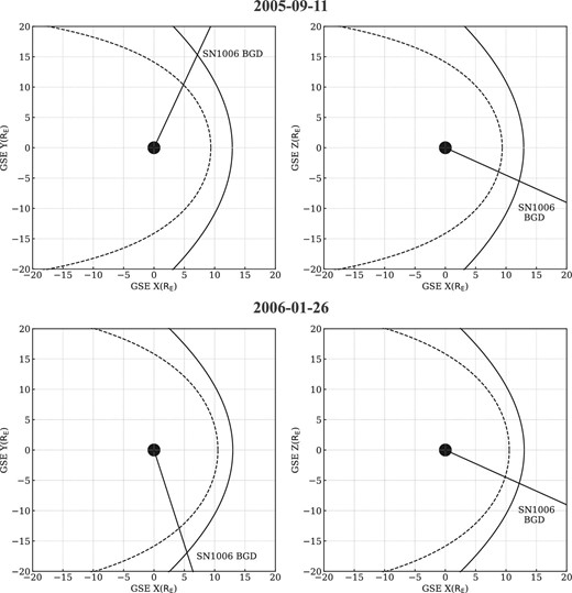
Line-of-sight directions in the GSE X–Y and X–Z planes during each Suzaku observation. The dashed and solid curves show the positions of the magnetopause and the bow shock at the ends of each observational period, respectively.
Suzaku (Mitsuda et al. 2007), the fifth Japanese X-ray satellite, has two types of main instruments: the X-ray Imaging Spectrometer (XIS; Koyama et al. 2007) and the Hard X-ray Detector (HXD; Takahashi et al. 2007). Suzaku has four XISs, each of which is an X-ray charge-coupled device (CCD) and works as the focal-plane detector of the X-Ray Telescope (XRT; Serlemitsos et al. 2007) for each. Three of the four XISs are front-illuminated CCDs (FI CCDs: XIS 0, XIS 2, XIS 3), whereas the other is a back-illuminated CCD (BI CCD: XIS 1). These X-ray CCDs have a relatively low and stable background level, owing to the low Earth orbit at 550 km altitude, and thus are suitable to detect SWCX emission. The observational parameters are summarized in table 1.
Summary of the observational parameters.
| Target name | SN 1006 SW BG | |
| Observation ID | 100019040 | 100019060 |
| Observation start (UT) | 2005-09-11 23:59 | 2006-01-26 17:16 |
| Effective exposure (ks) | 25.2 | 17.0 |
| Target coordinates (α, δ) (J2000.0) | (224|${_{.}^{\circ}}$|6550, −42|${_{.}^{\circ}}$|4005) | (224|${_{.}^{\circ}}$|6468, −42|${_{.}^{\circ}}$|4025) |
2.2 Solar activity and the geomagnetic field
Shortly before the first observation (i.e., in early September 2005), several successive X-class solar flares occurred even though it was close to solar-cycle minimum. In particular, a solar flare on 2005 September 7 was huge, classified as X17. Subsequently, X6- and X2-class flares erupted on September 9 and 10. These X-class flares entailed CMEs, as reported by Wang et al. (2006). We plot the time series of some selected parameters of the solar wind during the Suzaku observations in figure 2: the solar X-ray flux in the 0.1–0.8 nm band observed by the Geostationary Operational Environmental Satellite (GOES), the solar proton flux, the interplanetary magnetic field (IMF), the proton temperature, the plasma beta measured by WIND,1 and the Dst Index provided by the World Data Center for Geomagnetism, Kyoto, Japan. The gray points in the fourth panel of figure 2 indicate the temperature Texp expected from the solar wind velocity, calculated with the empirical formula in Lopez (1987).

From the top panel: solar X-ray light curve (0.1–0.8 nm), solar proton flux, IMF, proton temperature, plasma beta, and Dst Index. The gray points in the fourth panel indicate the temperature Texp expected from the solar wind velocity, calculated with the empirical formula in Lopez (1987). The orange areas indicate the periods of the Suzaku observations. The points plotted in the first and other panels are the average values over 5 min and 1 hour periods. The red shaded region shows the period of a lower plasma beta, starting on DOY 254 in 2005. (Color online)
At the beginning of day of year (DOY) 254 in 2005, the plasma beta decreased and the measured proton temperature dropped below Texp for a while, which followed discontinuous rises of the proton flux and proton temperature on DOY 254.0 (indicated by the red shaded region in figure 2). This phenomenon of a sudden drop in the plasma beta is a well-known indicator of an ICME front passing the observer’s location; the enhancements of the proton flux and temperature are due to a CME-driven front shock, whereas the low proton temperature and low plasma beta are caused by a magnetic cloud. This CME event was suspected to be caused by the X6 flare on September 9, which propagated from the Sun to the L1 point (where the GOES and WIND satellites reside) with a velocity of ∼1400 km s−1 (Wang et al. 2006). The mass of the CME was ∼1.6 × 10¹⁷ g, which makes it the most massive halo CME in the SOHO LASCO CME catalog (Gopalswamy et al. 2009).2 From these facts, we conclude that the Suzaku observation on 2005 September 11 was affected by the CME, whereas that on 2006 January 26 was not. Hereafter, we refer to the first and second Suzaku observation periods as the active and stable periods, respectively.
3 Analysis
We analyzed the data obtained with the XISs in both the active and stable periods. In our data reduction and analysis, we utilized the software included in the HEAsoft package version 6.25. We used the 3 × 3 and 5 × 5 editing modes for each of the XIS cleaned event data (filtered with the standard screening process;3 the processing script version was 3.0.22.43). Hereafter, quoted errors refer to 90% uncertainties unless otherwise noted.
3.1 XIS 1 images
We examined the data of the BI CCD (XIS 1), which is more sensitive than the FI CCDs (XIS 0, 2, and 3) in the soft (<1 keV) X-ray band, in which SWCX emission was mainly observed. Figure 3 shows XIS 1 images in the 0.4–2.0 keV band, without any background subtraction. The X-ray image of the active period was found to be clearly brighter than that of the stable period. Therefore, some additional X-ray emission must exist in the active period. We extracted the X-ray events from a circular region with a radius of |${8{^{\prime }_{.}}5}$|, excluding regions encompassing a few point sources (the hatched regions in figure 3). We confirmed the same X-ray enhancements in the FI CCDs (XIS 0, XIS 2, and XIS 3). Hence, the X-ray enhancement was not instrumental.
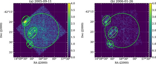
XIS 1 0.4–2.0 keV images in the active and stable periods. The color scale represents counts per pixel on a linear scale. The green circles show the region where we extracted the X-ray events (we excluded the hatched regions to remove the few point sources). (Color online)
3.2 Light curve
We extracted 480 s-bin light curves in the 0.4–2.0 keV and 2.0–10.0 keV bands for each XIS individually, and plot those of XIS 1 in figure 4. The 2.0–10.0 keV light curves of any of the XISs showed a distinctive X-ray enhancement between DOYs 255.35 and 255.40 (indicated by the orange-shaded area in figure 4). The timing coincided with a known M6-class solar flare (we can confirm the flare in the top panel of figure 2). Thus, we excluded the data in this time region in the following analyses. The 2.0–10.0 keV light curves of XIS 1 and 2 also showed a couple of sharp spikes with a shorter time scale than that of typical solar flares. However, the spikes did not appear in the XIS 0 or XIS 3 light curves. The inconsistency among the detectors implied that the spikes originated in something instrumental. To identify quantitatively the time regions of the instrumental spikes, we calculated the average and the standard deviation of the count rate in the 2.0–10.0 keV band, excluding the above-mentioned solar-flare period. Then, we selected the time bins in the light curves whose count rates were outside the 90% confidence interval as anomaly bins and excluded them in the following analyses. The excluded time bins are indicated with gray-shaded areas in figure 4.
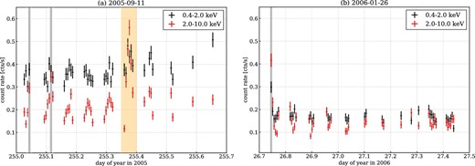
XIS 1 480 s-bin light curves in the (a) active and (b) stable periods in the (black) 0.4–2.0 keV and (red) 2.0–10.0 keV bands. The orange and gray shaded regions show the “flare” and a few rapid-rise periods, respectively, the data from which are excluded in the analyses. (Color online)
We found that the average count rate of the 0.4–2.0 keV light curves in the active period was apparently nearly twice as high as in the stable period (figure 4). We can also confirm the slight increase in the count rate of the 2.0–10.0 keV light curves, even excluding the solar-flare period (a possible origin of the increase is described in subsection 3.3).
3.3 Spectral fitting
We extracted the X-ray events from the data for each XIS and made BI (XIS 1) and FI (XIS 0 + XIS 2 + XIS 3) spectra in each observation period. The FI and BI spectra are binned with minima of 50 and 30 counts, respectively. Then we subtracted from each of the FI and BI spectra a simulated non-X-ray background (NXB) spectrum, which was created with xisnxbgen (Tawa et al. 2008). We made redistribution matrix files (RMFs) using xisrmfgen, and auxiliary response files (ARFs) using xissimarfgen (Ishisaki et al. 2007), under the assumption that the emission region is a circular region with a radius of 20′, given that the X-ray emission from the SN1006 background area appeared uniform. For the spectral fitting in this work, we used the XSPEC package (version 12.10.1).
3.3.1 Stable period
We analyzed the BI and FI spectra in the stable period with model fitting. In general, the NXB-subtracted X-ray spectrum of blank sky consists mainly of three components: the Galactic Halo (GH), the Local Hot Bubble (LHB), and the cosmic X-ray background (CXB; see, e.g., Kushino et al. 2002). The GH and LHB are thin thermal plasma (with typical temperatures of kT ∼ 0.3 keV and ∼0.1 keV, respectively). The CXB is now understood as the collective emission from unresolved active galactic nuclei (AGNs), and its emission is well approximated by a power law with a photon index of 1.41 (Kushino et al. 2002; De Luca & Molendi 2004).
Considering the composition, we first fitted the 2.0–5.0 keV band in the spectra, which is likely to be dominated by the CXB, with a power law with photon index fixed at 1.41. The normalization of the power law was determined to be 10.1 photons s−1 cm−2 keV−1 str−1 at 1 keV, which is consistent with the past result obtained with ASCA (Kushino et al. 2002). Then, we extended the energy ranges to 0.3–5.0 keV and 0.4–5.0 keV for the BI and FI spectra, respectively, for further analysis. We adopted two thin-thermal models and a power law (phabs*(vapec+powerlaw)+vapec in XSPEC). The parameters for the power-law component were fixed to the best-fitting values of the result described above in the model fitting. We note that the CXB and GH are affected by the Galactic hydrogen absorption, while the LHB is not. In our observed regions, the Galactic absorption column density was nH = 7.58 × 1020 cm−2 according to nh in the HEASoft package, which we adopted. We adopted the solar abundance table given by Anders and Grevesse (1989); the abundances of carbon, nitrogen, neon, and iron were set to be free, while those of the other elements were fixed to unity in our model fitting. All the abundance parameters were linked between the two thermal plasma models. Figure 5 shows the spectra and resultant best-fitting models, and table 2 summarizes the fitting results. The fitting was satisfactory with a reduced chi-squared of 1.06.
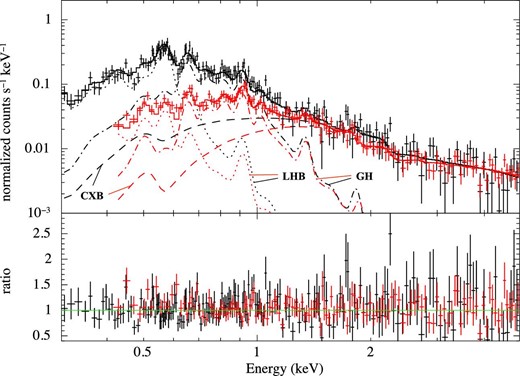
Spectra obtained with the (black) BI CCD and (red) FI CCDs in the stable period. The solid lines show the best-fitting models of the (dashed-dotted lines) GH, (dotted lines) LHB, and (dashed lines) CXB components. (Color online)
Results of the model fitting to the stable-period spectra.
| Model | Parameters | ||
|---|---|---|---|
| CXB (power law) | |$N_\mathrm{H}\ \mathrm{[10^{22} \, {\rm cm}^{-2}]}$| | 0.0758 (frozen) | |
| Photon index Γ | 1.41 (frozen) | ||
| Normalization* | 10.1 (frozen) | ||
| GH (vapec) | |$N_\mathrm{H}\ \mathrm{[10^{22} \, {\rm cm}^{-2}]}$| | 0.0758 (frozen) | |
| kT [keV] | |$0.297^{+0.013}_{-0.012}$| | ||
| Abundance† | C | |$1.26^{+0.76}_{-0.51}$| | |
| N | |$2.70^{+0.43}_{-0.40}$| | ||
| O | 1.00 (frozen) | ||
| Ne | |$1.26^{+0.20}_{-0.18}$| | ||
| Fe | |$0.45^{+0.10}_{-0.08}$| | ||
| Normalization‡ | |$32.2^{+3.5}_{-6.5}$| | ||
| LHB (vapec)§ | kT [keV] | |$0.130^{+0.016}_{-0.010}$| | |
| Normalization‡ | |$45.9^{+12.2}_{-8.9}$| | ||
| χ2/d.o.f. | 325.02 / 308 |
In units of photons s−1 cm−2 keV−1 str−1 at 1 keV.
These values are abundances with respect to the solar abundance.
In units of |$(4\pi )^{-1} D_{\mathrm{A}}^{-2} (1+z)^{-2} 10^{-14} \int n_{\mathrm{e}} n_{\mathrm{H}} dV$| steradian−1, where DA is the angular size distance to the source (cm), and ne and nH are the electron and hydrogen densities (cm−3), respectively.
Each abundance parameter is linked to that of the GH model.
3.3.2 Active period
We then analyzed the spectra in the active period to quantitatively evaluate the difference from the spectra in the stable period (hereafter, the spectra and best-fitting model of the latter are referred to as the 2006 spectra and model, respectively). Since these event data were extracted from an identical celestial region, we can remove the ambiguity due to the difference in the observational directions in the GSE coordinates. Following the method for the model fitting of the 2006 spectra, we first fitted the spectra of the active period in the 2.0–5.0 keV band only with a power law whose parameters were fixed to those of the 2006 model. We found that whereas the best-fitting parameters were consistent with those of the 2006 model with the FI-CCD spectrum, those of the BI-CCD spectrum showed an excess over the 2006 model. A similar excess in the BI-CCD spectrum was also reported in past SWCX studies with Suzaku (e.g., Fujimoto et al. 2007; Ezoe et al. 2011). Since the excess is only seen in the BI spectrum, it is probably due to particle backgrounds such as soft protons, as discussed by Ezoe et al. (2011). Regarding spectral fitting, Fujimoto et al. (2007) dealt with this feature by adding an unabsorbed power law to the blank-sky model. Accordingly, we added an unabsorbed power law to the 2006 model in order to address the discrepancy. Figure 6 shows the BI- and FI-CCD spectra and the 2006 model, plus the additional power law. Many Gaussian-like residuals, mainly below 2 keV, are still clearly visible, after including the additional power-law component.
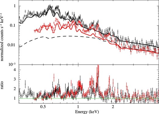
Spectra of the (black) BI CCD and (red) FI CCDs in the active period. The solid lines show the 2006 model and, for the BI-CCD spectrum only, an unabsorbed power law (dashed line). (Color online)
Then, we added Gaussian models one by one to the spectral model to eliminate the significant residuals and repeated the model fitting. In the fittings, the center energy and normalization of each Gaussian were allowed to vary but were set to be common (i.e., linked) between the BI- and FI-CCD spectra. Consequently, we obtained an acceptable fit by adding 17 Gaussian models. Figure 7 shows the best-fitting model with individual components. The residuals that are still seen in figure 7 may be due to systematic uncertainties of the line profiles. The parameters of the additional power law and Gaussians are summarized in tables 3 and 4. It should be noted that the additional power-law component is response-folded in our analysis. On the other hand, the soft proton contamination in the XMM-Newton observations can be approximated by a broken power-law model which is not folded through the detector response (Kuntz & Snowden 2008). We also confirm that our results shown in table 4 remain almost unchanged (even for the C lines, the decrease of the normalization is less than 30%), even if we substitute the response-unfolded power law for the response-folded one. The center energy of many of the Gaussians was found to be consistent with the energies of the characteristic X-rays from H-like or He-like ions of one of the relatively abundant elements. Notably, we identified the 459 eV line (C vi 4p to 1s), which is one of the main features of the SWCX (Fujimoto et al. 2007). Therefore, we concluded that the residuals in the fitting with the 2006 model were attributed to the SWCX emission.
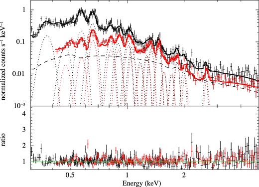
As figure 6, but the model contains an additional 17 Gaussians (dotted lines). The slight offsets between the Gaussians for the BI- and FI-CCD spectra are due to the difference in energy gain. (Color online)
Results of the model fitting to the active-period spectra.
| Model | Parameters | |
|---|---|---|
| 2006 model | Described in table 2 | |
| Additional power law | Photon index Γ | |$1.47^{+0.20}_{-0.21}$| |
| Normalization* | |$8.26^{+1.29}_{-1.00}$| | |
| Additional 17 Gaussians | Described in table 4 | |
| χ2/d.o.f. | 524.60 / 369 |
| Model | Parameters | |
|---|---|---|
| 2006 model | Described in table 2 | |
| Additional power law | Photon index Γ | |$1.47^{+0.20}_{-0.21}$| |
| Normalization* | |$8.26^{+1.29}_{-1.00}$| | |
| Additional 17 Gaussians | Described in table 4 | |
| χ2/d.o.f. | 524.60 / 369 |
In units of photons cm−2 s−1 keV−1 str−1 at 1 keV.
Best-fitting parameters of the Gaussians and identification of the lines.
| Gaussian* | Center energy [eV] | Normalization† | fX‡ | Line identification |
|---|---|---|---|---|
| 1 | |$374^{+7}_{-10}$| | |$11.6^{+2.8}_{-3.1}$| | |$7.42^{+1.79}_{1.96}$| | C vi 2p to 1s (368 eV) |
| 2 | |$468^{+10}_{-10}$| | |$2.73^{+1.00}_{-1.00}$| | |$2.18^{+0.80}_{-0.80}$| | C vi 4p to 1s (459 eV) |
| 3 | |$571^{+6}_{-5}$| | |$7.81^{+1.58}_{-1.48}$| | |$7.59^{+1.54}_{-1.44}$| | O vii |
| 4 | |$656^{+2}_{-6}$| | |$9.86^{+0.86}_{-0.95}$| | |$11.0^{+1.0}_{-1.1}$| | O viii 2p to 1s (653 eV) |
| 5 | |$814^{+7}_{-6}$| | |$2.20^{+0.38}_{-0.36}$| | |$3.05^{+0.53}_{-0.50}$| | O viii or Fe xvii |
| 6 | |$895^{+8}_{-10}$| | |$1.78^{+0.32}_{-0.33}$| | |$2.71^{+0.48}_{-0.50}$| | Ne ix or Fe xviii |
| 7 | |$1008^{+11}_{-4}$| | |$2.01^{+0.30}_{-1.02}$| | |$3.45^{+0.51}_{-1.76}$| | Ne x 2p to 1s (1022 eV) |
| 8 | |$1060^{+18}_{-8}$| | |$1.21^{+0.62}_{-0.68}$| | |$2.19^{+1.11}_{-1.23}$| | Ne ix ? |
| 9 | |$1172^{+18}_{-19}$| | |$0.42^{+0.13}_{-0.14}$| | |$0.83^{+0.27}_{-0.27}$| | — |
| 10 | |$1270^{+10}_{-14}$| | |$0.72^{+0.15}_{-0.14}$| | |$1.55^{+0.32}_{-0.30}$| | — |
| 11 | |$1339^{+7}_{-7}$| | |$1.04^{+0.16}_{-0.16}$| | |$2.37^{+0.36}_{-0.37}$| | Mg xi |
| 12 | |$1468^{+5}_{-5}$| | |$1.26^{+0.15}_{-0.14}$| | |$3.15^{+0.37}_{-0.36}$| | Mg xii 2p to 1s (1473 eV) |
| 13 | |$1564^{+20}_{-17}$| | |$0.28^{+0.12}_{-0.12}$| | |$0.75^{+0.33}_{-0.32}$| | Mg xi |
| 14 | |$1722^{+22}_{-25}$| | |$0.23^{+0.12}_{-0.10}$| | |$0.69^{+0.35}_{-0.29}$| | Mg xii 3p to 1s (1745 eV) |
| 15 | |$1836^{+3}_{-4}$| | |$0.55^{+0.09}_{-0.12}$| | |$1.72^{+0.29}_{-0.38}$| | Si xiii |
| 16 | |$2006^{+27}_{-27}$| | |$0.31^{+0.11}_{-0.11}$| | |$1.04^{+0.39}_{-0.39}$| | Si xiv 2p to 1s (2006 eV) |
| 17 | |$2616^{+23}_{-23}$| | |$0.33^{+0.12}_{-0.12}$| | |$1.46^{+0.54}_{-0.53}$| | S xvi 2p to 1s (2623 eV) |
The width of the lines are fixed to 0.
In units of photons cm−2 s−1 str−1.
fX is energy flux in units of 10−13 erg s−1 cm−2.
4 Discussion
4.1 Significance of the sulfur line
In section 3, we evaluated the SWCX lines from several ions with 17 Gaussian models. Notably, we found a line at around 2.62 keV, the energy of which coincides with the S xvi Lyα line. No previous studies have reported a positive detection of a S xvi line from SWCX emission. Our detection is a significant discovery if it is genuinely a S xvi line. Here we discuss how plausible this might be.
SWCX emission is known to contain not only Heα and Lyα lines but also various lines caused by other transitions. In case of the 2.62 keV line, there is a possibility that this line is attributed to Si xiv Lyζ and Lyη, whose energies are at around 2.62 keV. In order to evaluate the contribution of the characteristic cascades, we incorporated a set of AtomDB Charge Exchange (ACX) models (Smith et al. 2014)4 instead of a set of simple Gaussians and fitted the spectra with the model to see how the residuals in figure 6 might be explained. The residuals in figure 6 can be mostly attributed to the characteristic lines from the seven elements carbon, oxygen, neon, magnesium, silicon, sulfur, and iron (table 4). Accordingly, our new model consists of, in addition to the continuum of the 2006 model and an additional power law, seven vacx models (the variable abundance version of the ACX model), each of which represents the charge exchange emission from a separate element (note that we set the other abundances to a fixed value of 0). Since we have no way to measure the absolute hydrogen abundance in the plasma (the vacx model has no continuum), only the relative abundances can be obtained in principle. Therefore, we linked the normalizations of all the vacx components and fixed the oxygen abundance to unity in the fitting. We performed model fitting of the spectra in the active period and obtained the relative abundances of the six elements to the oxygen and ion population Tz, which indicates the ion population as though it were in collisional ionization equilibrium created by electrons at temperature Tz. These ion populations derived by SWCX do not necessarily coincide with the real ion population; our observation in the X-ray band is only sensitive to highly charged ions.
Table 5 lists the fitting results, and figure 8 shows the best-fitting model. The relative abundances of the elements to oxygen are found to be close to the solar abundances, except for carbon, which is significantly higher (carbon-rich) than the solar abundance. We conjecture that the apparent high carbon abundance is probably due to an effect of contamination from the heliospheric SWCX emission. We also note that the tendency for low abundances of silicon and sulfur are consistent with another observational result of the same solar flare with Suzaku, using Earth’s X-ray albedo (Katsuda et al. 2020). This result, where the X-rays from the Si xiv line are fully taken into account, implies that the ACX model of sulfur is needed to explain the observed spectra at a confidence level of more than 3 σ. Hence, we conclude that the detected 2.62 keV line is S xvi Lyα, which is the first detection of the line from SWCX emission.
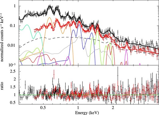
As figure 7, but the model has seven ACX models instead of Gaussians (only those for the BI spectrum are depicted). The line color distinguishes the element of each ACX model: (green) C, (orange) O, (gray) Fe, (blue) Ne, (lime green) Mg, (red) Si, and (magenta) S. (Color online)
Best-fitting parameters with the 2006 model plus additional power law and seven ACX models.
| Model | Parameters | ||
|---|---|---|---|
| 2006 model | Described in table 2 | ||
| Photon index Γ | Normalization* | ||
| Additional power law | |$1.21_{-0.36}^{{+0.35}}$| | |$6.33_{-1.72}^{{+1.74}}$| | |
| Abundance† | Ion population Tz [keV] | ||
| vacx | C | >4.89 | |$0.075_{-0.005}^{+0.008}$| |
| O | 1 (fixed) | |$0.210_{-0.009}^{+0.010}$| | |
| Ne | |$1.22_{-0.24}^{+0.28}$| | |$0.526_{-0.033}^{+0.046}$| | |
| Mg | |$1.67_{-0.33}^{+0.41}$| | |$0.988_{-0.098}^{+0.146}$| | |
| Si | |$0.729_{-0.300}^{+0.371}$| | |$1.18_{-0.20}^{+0.39}$| | |
| S | |$0.619_{-0.320}^{+0.362}$| | >2.35 | |
| Fe | |$1.39_{-0.49}^{+0.61}$| | |$1.16_{-0.07}^{+0.12}$| | |
| χ2/d.o.f. | 595.56/389 | ||
In units of photons cm−2 s−1 keV−1 str−1 at 1 keV.
These values are abundances with respect to solar.
4.2 Correlation with the CME
We have shown that Suzaku detected various kinds of SWCX lines during the active period. Given that indicators of an ICME were observed by in situ measurements at the same time, this SWCX emission is likely to be associated with the ICME. Some past similar studies examined the correlation between the observed X-ray light curves and arrival of an ICME to establish their association (e.g., Ezoe et al. 2010; Ishi et al. 2019). However, since the observed X-rays during the observation in the active period did not show much time fluctuation, the method would yield nothing significant in our case. Instead, we evaluated the plasma metal abundance in the same way as in a previous study of spectrally rich ICME-driven SWCX emission (Carter et al. 2010), which took account of 33 emission lines from carbon, nitrogen, and oxygen, of which the emission cross-sections are listed in table 2 of Bodewits et al. (2007). The normalization of the line with the largest cross-section in each ion species was set as a free parameter in the fitting, while those of the other lines were determined according to the relative emission cross-sections. In our case, we adopted the cross-section at the solar wind speed of 1000 km s−1, which is close to the average speed during our observation period (915 km s−1). As for the other line parameters, we added Gaussians for the ions at the fixed transition energies which were detected by Carter, Sembay, and Read (2010) and for S xvi at 2.62 keV. Then, we fitted the spectra in the active period with the model. Table 6 summarizes the fitting result, and figure 9 shows the best-fitting spectra. We find that this model can also explain the observed spectra.
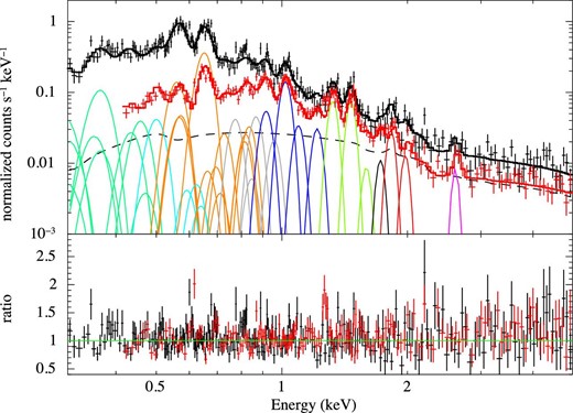
As figure 6, but the model additionally contains the same SWCX model as Carter, Sembay, and Read (2010) and the S xvi line (only those for the BI spectrum are depicted). The center energy of each Gaussian is fixed to the transition energy of each ion. The line color shows the type of the element species: (green) C, (cyan) N, (orange) O, (gray) Fe, (blue) Ne, (lime green) Mg, (black) Al, (red) Si, and (magenta) S. (Color online)
Best-fitting parameters in model fitting with the fixed-center-energy Gaussians.
| Gaussian* | Center energy [eV] | Normalization† | Line identification |
|---|---|---|---|
| 1 | 299 | |$33.6^{+20.0}_{-20.0}$| | C v |
| 2 | 367 | |$8.71^{+2.87}_{-2.89}$| | C vi |
| 3 | 420 | — | N vi |
| 4 | 500 | |$1.30^{+0.86}_{-0.87}$| | N vii |
| 5 | 561 | |$5.15^{+1.03}_{-1.04}$| | O vii |
| 6 | 653 | |$9.57^{+0.93}_{-0.93}$| | O viii |
| 7 | 730 | |$0.60^{+0.47}_{-0.47}$| | Fe xvii |
| 8 | 820 | |$0.52^{+0.43}_{-0.43}$| | Fe xvii |
| 9 | 870 | |$0.90^{+0.38}_{-0.38}$| | Fe xviii |
| 10 | 920 | |$1.04^{+0.39}_{-0.39}$| | Ne ix |
| 11 | 960 | |$0.39^{+0.29}_{-0.29}$| | Fe xx |
| 12 | 1022 | |$2.53^{+0.26}_{-0.26}$| | Ne x |
| 13 | 1100 | |$0.60^{+0.16}_{-0.16}$| | Ne ix |
| 14 | 1220 | |$0.56^{+0.14}_{-0.14}$| | Ne x |
| 15 | 1330 | |$1.32^{+0.15}_{-0.15}$| | Mg xi |
| 16 | 1470 | |$1.31^{+0.15}_{-0.15}$| | Mg xii |
| 17 | 1600 | |$0.20^{+0.11}_{-0.11}$| | Mg xi |
| 18 | 1730 | |$0.26^{+0.11}_{-0.11}$| | Al xiii |
| 19 | 1850 | |$0.69^{+0.15}_{-0.15}$| | Si xiii |
| 20 | 2000 | |$0.30^{+0.12}_{-0.12}$| | Si xiv |
| 21 | 2623 | |$0.32^{+0.12}_{-0.12}$| | S xvi |
The width of the lines are fixed to 0.
In units of photons cm−2 s−1 str−1.
From the fitting result, we calculate the energy flux of each ion species and plot the energy flux ratios of the lines to the O viii line (654 eV) in figure 10. In the figure, we also plot for reference the results by Carter, Sembay, and Read (2010) and the calculated energy flux ratio for the heliospheric SWCX, where the same cross-sections and slow equatorial solar wind abundance as given by Schwadron and Cravens (2000) are assumed. Our result is found to roughly agree with that of the ICME-driven case (Carter et al. 2010) except for carbon, nitrogen, and oxygen. We conjecture that the discrepancies with regard to carbon, nitrogen, and oxygen are due to a potential increase of the heliospheric SWCX component, given that the intensities of the heliospheric SWCX can be different between the stable and active periods. The detection of the lines from Fe xvii, Fe xviii, and Fe xx indicates the existence of highly ionized iron; it is consistent with the characteristic of the iron state in ICMEs (summarized in Zurbuchen & Richardson 2006), whereas the stable slow solar wind barely has such ions. These features also support that this event is ICME driven.
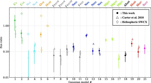
Energy flux ratio of the line to the O viii line (654 eV). The circles and triangles indicate our results and those by Carter, Sembay, and Read (2010), respectively. The diamonds indicate the heliospheric SWCX case calculated with the slow solar wind abundance given by Schwadron and Cravens (2000). (Color online)
The first detection of the emission line from S xvi suggests this to be the most spectrally rich SWCX event ever reported (note that there is a possibility that the energy range above 2 keV was not fully investigated in some of the SWCX studies and that line features were overlooked). The flare which triggered the ICME associated with the event is of the X6 class, which is one of the most intense flares in the ICME-driven SWCX samples. This fact may suggest that the solar flare magnitude is related to the ionization states in the ICME, as pointed out by Reinard (2005).
4.3 SWCX as a new tool to detect highly ionized ions in the solar wind
From the eruption at the low corona to propagation to interplanetary space, a CME evolves and its properties change. In particular, the CME plasma in the early phase of the evolution (up to a few R⊙) undergoes a continuous heating process; signs of heating have been observed by the Ultraviolet Coronagraph Spectrometer (UVCS) onboard SOHO, which provides valuable information to constrain the heating model (e.g., Akmal et al. 2001; Landi et al. 2010). Even though the evolution of CMEs has been studied extensively with observations and simulations for a few decades, the heating mechanism still remains an open question.
The ionic charge state distribution in an ICME is also an effective tool to diagnose its plasma state. As CME ejecta are adiabatically expanding toward the outer region, the density of the ejecta gradually decreases. Once the density has dropped sufficiently low, the ejecta become collisionless and then the ionization state of each ion is fixed at the specific distance from which no ionization or recombination takes place (the so-called “freeze-in height”) while it is transferred away to the heliosphere. Hence, the ionization state of ions in an ICME preserves its post-heating plasma information at the freeze-in height. This implies that in situ measurements of these ions can also constrain the evolution history of CMEs, as discussed by, e.g., Gruesbeck et al. (2011) and Rivera et al. (2019).
The ionic charge state distribution in ICMEs has been repeatedly observed with the Solar Wind Ion Composition Spectrometer (SWICS) onboard the Advanced Composition Explorer (Gloeckler et al. 1998). The SWICS can obtain information on the plasma composition using three observable parameters for each ion count (energy per charge, time of flight, and residual energy). The SWICS data are publicly distributed and serve as the standard dataset in this field, containing information on several ions (the gray regions in figure 11). Although the SWICS is able to detect a wide range of energy, some ion species are deliberately excluded from the public standard dataset due to the complexity of the data analyses. Gilbert et al. (2012) reported that they detected low-charged ions in ICMEs with a new analysis method, extending the observed parameter space of the ion species in ICMEs (the black hatched regions in figure 11). However, it is still difficult for the SWICS to observe some H-like or He-like ions due to poor statistics.
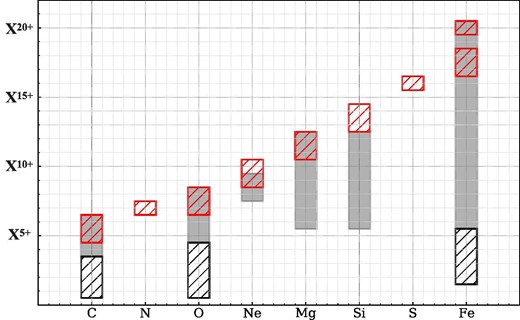
Detectable charge states of C, N, O, Ne, Mg, Si, S, and Fe with the currently available observations. The gray shaded areas show the available charge state distributions in the SWICS standard dataset. The red and black hatched areas show the ranges obtained in our SWCX observation and Gilbert et al. (2012), respectively. (Color online)
The SWCX emission from a variety of highly charged ions provides information on the plasma composition (see section 1). In particular, some ICME-driven SWCX events have emission lines from ions that are hardly detected by SWICS but can be detected with data similar to those used in this work. Although there is a downside in our method that an accurate cross-section of the SWCX is required to obtain the absolute flux of each ion, we suggest that ICME-driven SWCXs can provide a unique opportunity to detect these highly charged ions in ICMEs. So far, in situ measurements have been the only way to obtain the physical parameters useful in studying the plasma state at the freeze-in point. The data and method used in this work serve as a new and complementary method for this.
Though Suzaku and XMM-Newton have made great contributions to SWCX research, the energy resolutions of the spectroscopic imagers onboard these satellites are not sufficiently high to resolve complex line structures, especially below 1 keV. Some of the planned future X-ray astronomical satellites are expected to address this issue much better. The X-Ray Imaging and Spectroscopy Mission (XRISM), scheduled to be launched in Japanese fiscal year 2022, has a non-dispersive soft X-ray spectrometer with a high spectral resolution (full width at half maximum <7 eV at 6 keV) over the 0.3–12.0 keV band-pass (Tashiro et al. 2020). Spectroscopy with XRISM can reveal the line structure for the first time. Also, the Advanced Telescope for High-ENergy Astrophysics (Athena) can also contribute to the study of ICMEs through observations of the SWCX if it is put at the L1 Lagrange point.
Finally, charge exchange processes happen not only in our solar system but also in supernova remnants, starforming galaxies, and galaxy clusters. Hence, understanding the physical process is important in a wide field of astrophysics, as discussed by the XRISM Science Team (2020).
5 Conclusions
We analyzed the SN1006 background data observed with Suzaku on 2005 September 11, using another observation of the same field at a different epoch as the reference. We found that the data contained an additional soft-X-ray component compared with the reference data, which were taken when the solar activity was stable. With spectral model fitting, we revealed the additional component to be multiple emission lines, which can be explained as SWCX emission. The observation period coincided with the passage of an ICME associated with an X6 flare that had happened shortly before the Suzaku observation. The coincidence, as well as the fact that the characteristics of the emission lines were consistent with those of ICME-driven SWCX events reported in the past, strongly imply that this SWCX event was ICME driven. Notably, we detected an emission line from S xvi with a confidence level of more than 3 σ for the first time as one from SWCX, which suggests that this is the most spectrally rich SWCX event ever reported. Note that some of the ions, including highly ionized sulfur, that we detected cannot be detected by currently available in situ solar wind monitoring due to poor statistics. We propose that SWCX is a new tool for diagnosing ICME plasma, understanding which is important not only in studying X-ray diffuse background but also understanding the coronal heating mechanism.
Acknowledgements
The authors gratefully acknowledge the use of data obtained from the Suzaku and ACE satellites, NASA/GSFC’s Space Physics Data Facility’s OMNIWeb service, and the SOHO LASCO CME catalog. The CME catalog is generated and maintained at the CDAW Data Center by NASA and The Catholic University of America in cooperation with the Naval Research Laboratory. SOHO is a project of international cooperation between ESA and NASA. This work was supported by Japan Society for the Promotion of Science (JSPS) KAKENHI Grant Nos. 20J20685 (KA); 20H00175 (HM); 18J20523 (TY); 19K21884, 20H01941, 20H01947, 20KK0071 (HN); 18K18767, 19H00696, 19H01908, 20H00176 (KH); 20K20935 (SK); 19J20910 (DI); and 20H00177 (YE). This work was also partly supported by Mitsubishi Foundation Research Grant in the Natural Sciences 201910033 (KH); Leading Initiative for Excellent Young Researchers, MEXT, Japan (SK); and Toray Science and Technology Grant (YE).
Footnotes
We obtained the data from OMNIWeb 〈https://omniweb.gsfc.nasa.gov〉.
