


Abstract
We present our analysis of the Suzaku data of U Geminorum (U Gem) from 2012 both in quiescence and outburst. Unlike SS Cygni (SS Cyg), the hard X-ray flux of U Gem is known to increase at times of optical outburst. A sophisticated spectral model and reliable distance estimate now reveal that this can be attributed to the fact that the mass accretion rate onto the white dwarf (WD) does not exceed the critical rate that causes the optically thin to thick transition of the boundary layer. From comparison of the X-ray and optical light curves, the X-ray outburst peak seems to be retarded by 2.1 ± 0.5 d, although there remains uncertainty in the X-ray peak identification, due to short data coverage. The larger delay than SS Cyg (0.9–1.4 d) also supports the lower accretion rate in U Gem. A fluorescent iron 6.4 keV emission line bears significant information about the geometry of the X-ray-emitting hot plasma and the accretion disk (AD) that reflects the hard X-ray emission. Our reflection simulation has shown that the optically thick AD is truncated at a distance of 1.20–1.25 times the white dwarf radius (RWD) in quiescence, and the accreting matter in the disk turns into the optically thin hard-X-ray-emitting plasma at this radius. In outburst, on the other hand, our spectral analysis favors the picture that the optically thick disk reaches the WD surface, although disk truncation can take place in the region of <1.012 RWD. From the profile of the 6.4 keV line, we have also discovered that the accreting matter is heated up close to the maximum temperature immediately after the matter enters the boundary layer at the disk truncation radius. This is consistent with the fact that the hard X-ray spectra of dwarf novae, in general, can be well represented with the cooling flow model.
1 Introduction
A cataclysmic variable (CV) is a semi-detached binary system consisting of a late-type star and a white dwarf (WD) whose optical brightness fluctuates on a time scale of seconds to years. A dwarf nova (DN), one of the CV sub-categories, shows optical outbursts typically with ΔmV = 2–5, lasting a week to several months, with intervals of 10 d to tens of years.
Of the DNe, U Gem and SS Cyg belong to the U Gem subtype, the orbital period of which is longer than 3 hr. U Gem was discovered in 1855 and is one of the most extensively observed DNe. However, previous studies have reported that U Gem and SS Cyg show different behavior of X-ray radiation above 2 keV at the onset of the optical outburst state. As the mass accretion rate increases, the extreme ultraviolet (EUV) flux of SS Cyg suddenly increases simultaneously with the abrupt hard X-ray flux suppression (Wheatley et al. 2003), whereas in the case of U Gem, the hard X-ray flux increases with the EUV flux (Mattei et al. 2000). This difference is thought to originate based on whether the mass transfer rate through the accretion disk (AD) exceeds the critical value (1016 g s−1; Pringle & Savonije 1979), above which the optically thin hot plasma formed in the boundary layer (BL) turns into an optically thick state. Although some suggestions against this conclusion have been proposed (e.g. Ducci et al. 2016), Wheatley, Mauche, and Mattei (2003) confirmed that in SS Cyg outbursts, the mass accretion rate in the BL exceeds this value. Alternatively, in the case of U Gem, a similar quantitative evaluation has not yet been reported.
It is known that there is a significant geometric difference between the X-ray-emitting hot plasma of SS Cyg in quiescence and outburst. In quiescence, the plasma is located in the BL formed between the WD surface and the AD inner edge, whereas in outburst, the BL becomes optically thick, emitting EUV radiation, and the hot plasma is believed to distribute above the AD (Ishida et al. 2009). It is expected from the U Gem X-ray behavior that the U Gem plasma geometry in outburst is similar to that of SS Cyg in quiescence, which should be validated from observations.
In this study we investigate the state of the X-ray-emitting hot plasma, with a primary focus on the mass accretion rate, by means of spectral analysis, and the geometry of the plasma, by comparing an observed iron 6.4 keV fluorescence line with spectral simulations of reflection from the WD and AD surfaces. For this investigation we utilize the Suzaku archival data of U Gem taken in 2012. The paper is organized as follows. In section 2 we describe how the observations and data reductions have been performed. In section 3, we explain the analysis method in detail. We have obtained the U Gem spectral parameters and derived the mass accretion rate through the BL in both quiescence and outburst. The reflection simulation is presented here in full. Sections 4 and 5 are dedicated to discussion and conclusion, respectively.
2 Observations and data reduction
2.1 Observations
In figure 1, we show an optical light curve covering our U Gem observations taken from the of American Association of Variable Star Observers (AAVSO) home page.1 The hatched stripes (a) and (b) indicate the windows of the Suzaku outburst and quiescence observations, respectively. The basic U Gem parameters found in previous research are shown in table 1.
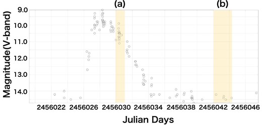
Optical light curve of U Gem in the V band from AAVSO. Stripes (a) and (b) indicate the Suzaku observation window for outburst and quiescence, respectively. (Color online)
We used Suzaku U Gem archival data in quiescence and outburst. Suzaku is Japan’s fifth X-ray astronomy satellite, and it has three major instruments: the X-Ray Spectrometer (XRS: Kelley et al. 2007), the X-ray imaging spectrometer (XIS: Koyama et al. 2007), and the hard X-ray detector (HXD: Takahashi et al. 2007; Kokubun et al. 2007). In this study we used data taken with the XIS and the HXD only, because the X-ray microcalorimeter, and hence XRS data, was lost on 2005 August 8 due to evaporation of the He coolant. The XIS consists of four X-ray CCD cameras (XIS 0, XIS 1, XIS 2, XIS 3), where XIS 1 adopts a back-illuminated charge-coupled device (BI-CCD) while the others consist of front-illuminated CCDs (FI-CCD). Note that XIS 2 has not been operational since 2006 November, probably because of a micrometeorite or space debris impact. The XIS has sensitivity in the energy range 0.2–12.0 keV, and its energy resolution is 130 eV at 6 keV. Each CCD camera has a focusing X-ray mirror XRT (Serlemitsos et al. 2007) whose focal length is 4.75 m. The HXD is a non-imaging instrument covering the energy band 12–600 keV, with hybrid detectors composed of PIN diodes and a GSO scintillator. The Suzaku observations of U Gem in outburst and quiescence were performed on 2012 April 12 and 2012 April 24, respectively. The observation log is summarized in table 2.
Observation log of U Gem.
| Seq. # | State | Observation date | Detector | Exposure (ks) | Count rate (s−1)* |
|---|---|---|---|---|---|
| 407035010 | Outburst | 2012 Apr 12 | XIS | 50.3 | 1.149 ± 0.003 |
| HXD | 44.4 | 0.009 ± 0.002 | |||
| 407034010 | Quiescence | 2012 Apr 24 | XIS | 119.1 | 0.491 ± 0.001 |
| HXD | 93.1 | 0.010 ± 0.002 |
Count rate in the 1.0–10 keV (XIS 0 + XIS 1 + XIS 3) and 15–30 keV bands (PIN) with 1 σ statistical errors.
2.2 Data reduction
We used the HXD data in the 15–30 keV band. For the XIS, on the other hand, we restricted our analysis to the 1.0–10 keV band. This is because the band below ∼1 keV is modified by photoelectric absorption of the interstellar matter and contains numerous emission lines. These sometimes make spectral modeling complicated and can easily raise a large systematic error, which can propagate to the higher-energy band, which is the our current focus of interest. In data reduction, we used the HEADAS software package,2 version 6.26. We followed standard data screening procedures for both XIS and HXD. We extracted source events within the 4′-radius circle centered on the U Gem image brightness peak, and the background events from the outer 4′–8′ annulus separately for each XIS module. Light curves of XIS with a binning of 128 s are shown in figure 2.
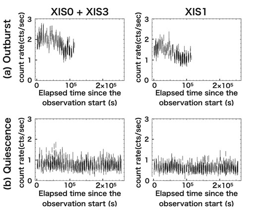
Background-subtracted XIS light curves of U Gem in outburst (top) and quiescence (bottom) in the 1.0–10 keV band, binned at 128 s for both. The left panels show the light curves of the combined FI-CCD cameras, whereas the right panels show those of the BI-CCD camera. The time origins are JD 2456029 21:51:10 and JD 2456042 1:31:43, respectively.
Although the data span only one day [see stripe (a) in figure 1], which is far from covering the entire optical outburst cycle, our outburst light curves seem to catch the X-ray intensity peak, which occurs at ∼20000 s from the time origin, which is JD 2456029.9. From figure 1, on the other hand, the optical outburst peaks at around JD 2456028.0. Consequently, the X-ray outburst peak is retarded from the optical one by roughly 2.1 d with a conservative error of ∼0.5 d. We remark that in SS Cyg, the hard X-ray rise of the outburst occurs about 0.9–1.4 d after the optical rise (Wheatley et al. 2003). Although the peak identification of our X-ray light curves is not decisive, the delay is larger in U Gem. This may reflect a difference in the density wave propagation velocity associated with the difference in the mass accretion rate. Because U Gem was weak in the HXD band during both quiescence and outburst (table 2), it is impossible to draw light curves in the 15–30 keV band.
3 Analysis
3.1 Estimate of the mass accretion rate with spectrum analysis
3.1.1 Spectrum analysis methods
3.1.2 Spectrum analysis result
We fitted the model “tbabs × (reflect × cevmkl + gauss)” explained above to the U Gem spectra in quiescence and outburst separately. We used both XIS and HXD data, and completed the fitting in the 1–30 keV band. The hydrogen column density (NH/1022 cm−2) is fixed based on ultraviolet observations (Long et al. 1996). The covering fraction of the reflector (Ω/2π) is fixed at 1.5 based on the result for SS Cyg (Ishida et al. 2009). This reflects that the BL is confined in a tight space between the WD and the edge of the AD (Ishida et al. 2009). The metal abundance of the elements lighter than Fe, which is mainly determined by oxygen abundance, is fixed at 0.58, based on the result of a simultaneous fitting of the outburst and quiescence spectra. The solar abundance table of Anders and Grevesse (1989) was adopted. The results of the fit are shown in panels (a-1) and (b-1) of figure 3. The best-fitting parameters are summarized in table 3, from which we have calculated the bolometric flux of the hard X-ray emission. In doing this, we set the solid angle of the reflector equal to zero after the best fit is obtained, to exclude the flux reflected off the WD surface and the AD. The resultant mass accretion rate is |$\dot{M}=1.87\times 10^{14}$| g s−1 in outburst and |$\dot{M}=0.89\times 10^{14}$| g s−1 in quiescence. Because |$\dot{M}$| is smaller than the critical value (1016 g s−1), this result is consistent with the conjecture that the BL does not turn into the optically thick state even during the outburst phase, and the gravitational energy released in the BL is emitted in the hard X-ray band.
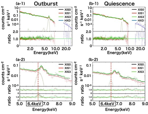
Fitting results to the combined XIS and HXD spectra of the outburst and quiescent states in the 1.0–30.0 keV band (a-1, b-1). Panels (a-2) and (b-2) are magnifications of the 5.0–9.0 keV band, showing the iron line spectra. Black, red, green, and blue are used for XIS 0, XIS 1, XIS 3, and HXD, respectively. The third rows of panels (a-2) and (b-2) show the data residuals from the model with the normalization of the lines being set equal to zero. The significance of the lines is 8.0 σ and 4.8 σ for outburst and quiescence, respectively. (Color online)
Result of the spectral fitting.*
| Parameter | Outburst | Quiescence |
|---|---|---|
| N H |$/$|1022 cm−2† | 0.0031 (fixed) | |
| Ω/2π‡ | 1.5 (fixed) | |
| T max (keV) | |$11.6_{-0.6}^{+0.7}$| | |$15.9_{-1.2}^{+1.1}$| |
| α | |$1.17_{-0.08}^{+0.10}$| | |$1.16_{-0.07}^{+0.07}$| |
| Z He (Z⊙)§ | 1.00 (fixed) | |
| Z C (Z⊙)§ | 1.00 (fixed) | |
| Z N (Z⊙)§ | 1.00 (fixed) | |
| Z O (Z⊙)§ | 0.58 (fixed) | |
| Z Ne (Z⊙)§ | 2.02 (fixed) | |
| Z Na (Z⊙)§ | 1.00 (fixed) | |
| Z Mg (Z⊙)§ | 1.11 (fixed) | |
| Z Al (Z⊙)§ | 1.00 (fixed) | |
| Z Si (Z⊙)§ | 1.29 (fixed) | |
| Z S (Z⊙)§ | 1.85 (fixed) | |
| Z Ar (Z⊙)§ | 1.00 (fixed) | |
| Z Ca (Z⊙)§ | 1.00 (fixed) | |
| Z Fe = ZNi (Z⊙)| | |$0.83_{-0.06}^{+0.06}$| | |$0.89_{-0.05}^{+0.05}$| |
| LineE (keV) | |$6.50_{-0.04}^{+0.03}$| | |$6.40_{-0.05}^{+0.04}$| |
| Sigma (keV) | |$0.12_{-0.03}^{+0.02}$| | |$0.06_{-0.06}^{+0.06}$| |
| |$\chi ^{2}_{\rm red}$| (dof) | 1.51(807) | 1.20(801) |
| L bol (×1031 g cm2 s−3) | 2.64 | 1.26 |
| |$\dot{M}$| (g s−1) | 1.87 × 10¹⁴ | 0.89 × 10¹⁴ |
Errors obtained using the error command included in the “xspec.”
Hydrogen column density is fixed based on ultraviolet observations (Long et al. 1996).
Covering fraction of the reflector is fixed at 1.5 based on the result for SS Cyg (Ishida et al. 2009).
Metal abundances (other than Fe, Ni) are fixed respectively based on the result of a simultaneous fitting of the outburst and quiescence spectra.
The solar abundance table of Anders and Grevesse (1989) is adopted.
3.2 Plasma geometry estimate by reflection simulations
3.2.1 Reflection simulation
In the previous section we showed that the BL of U Gem, unlike that of SS Cyg, can be considered optically thin even during the outburst phase, based on the fact that the observed mass accretion rate is less than the critical value. It is suggested, however, that the fluorescent iron line profile at 6.4 keV is somewhat different between the two states (table 3); the line becomes broad and its central energy shifts to ∼6.5 keV in the outburst state, while it is narrower and the central energy is consistent with 6.4 keV in the quiescent state. These 6.4 keV line characteristics are demonstrated in panels (a-2) and (b-2) of figure 3. To show the significance of these lines, in the third rows of panels (a-2) and (b-2) we show the residuals of the data above the model with the line normalization being set equal to zero. The significance of the 6.4 keV line is 8.0 σ and 4.8 σ for outburst and quiescence, respectively.
The 6.4 keV line originates from a cold reflecting material, such as the surfaces of the WD and the AD, via fluorescence. The former produces a narrow line, whereas the latter emits a broad line associated with the Kepler motion of the inner AD. Utilizing the line profile, we can therefore estimate the geometry of the X-ray-emitting hot plasma in relation to the reflection material, namely the WD and AD. Hence, we attempted to carry out a reflection simulation with various geometrical parameters of the plasma. In this simulation, using the Monte Carlo method, we follow each X-ray photon originating from the hot plasma throughout a sequence of interactions until it escapes from the reflecting material, is absorbed within the reflecting material, or its energy drops below 1 keV (Hayashi et al. 2018). The WD as a reflector is a cold and static sphere with the same metal abundance as the hot plasma. The hot plasma is a torus located at a distance Rp from the center of the WD and at Dv from the AD plane. Note that the torus cross-section equals zero. We assume the cevmkl model as the intrinsic emission spectrum from the hot plasma. The simulation considers photoelectric absorption, coherent scattering, and incoherent scattering as the interactions of the photons from the plasma with the reflecting matter. In addition to Rp and Dv, we have one more variable parameter, Rc–i, which is the distance from the center of the WD to the edge of the AD (figure 4). Examples of resultant spectra are shown in figure 5. We set Rc–i equal to 1.1 RWD and performed three simulations with Rp = 1.01 RWD, 1.1 RWD, and 1.2 RWD. In the case of Rp = 1.01 RWD, the 6.4 keV fluorescent iron line is narrow. The line is dominated by the WD surface component because of its larger solid angle over the plasma than that of the AD. Conversely, in the other two cases the 6.4 keV line has a broad double-horn profile associated with the Kepler motion of the inner AD. In the case of Rp = 1.2 RWD, the intensity of the broad double-horn component is larger than the 1.1 RWD case relative to the narrow component, whereas the energy separation of the horns is smaller than that of the 1.1 RWD case. This is because the solid AD angle viewed from the hot plasma is larger in the case of Rp = 1.2 RWD, whereas the plasma looks at the AD area with less velocity. In this way, the 6.4 keV line profile is sensitive to the hot plasma geometry. Hereafter we represent the parameter values Rp, Rc–i, and Dv in units of the WD radius RWD.
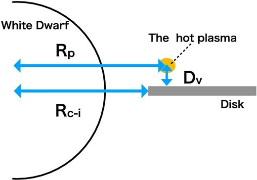
Geometrical parameters of our reflection simulation. Hot plasma is a torus located at a distance Rp from the center of the WD and Dv from the AD plane. Rc–i is the distance from the center of the WD to the inner edge of the AD. (Color online)
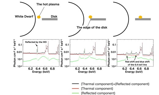
Examples of profiles of the fluorescent iron line at 6.4 keV from our reflection simulations. We fixed Rc–i at 1.1 RWD and varied Rp at 1.01 RWD (left), 1.1 RWD (center), and 1.2 RWD (right). In the case of Rp = 1.01 RWD, the 6.4 keV line is dominated by the component from the WD surface because of its larger solid angle over the plasma than that of the AD. Alternatively, in the other two cases a double-horn component gradually dominates the line spectrum. The energy separation of the horns is larger in the Rp = 1.1 RWD case because the plasma is closer to the inner edge of the AD, where the Keplerian velocity is the largest. The equivalent width of the double-horn component is larger in the case of Rp = 1.2 RWD because the solid angle of the disk is larger. (Color online)
Our simulation procedure to constrain these parameters through spectrum fitting is as follows:
We try to fit the spectrum with the model tbabs × (reflect × cevmkl + gaussian), which is the same model as used in the spectrum analysis (subsection 3.1). This aims at obtaining a first-order approximation of the hot plasma emission spectrum model.
Using Tmax (maximum temperature of the plasma) and ZFe (iron abundance) from the previous step, we run the simulation to obtain a spectrum that is reflected off the WD and the AD under the assumed values of Rc–i, Rp, and Dv.
Using the reflection spectrum calculated in the previous step, we try to fit the observed spectrum to find a new pair of Tmax and ZFe.
We return to Step 2 with the new values of Tmax and ZFe. We repeat Steps 2–4 until we minimize the χ2 value.
3.2.2 Evaluation of the outburst spectra with the simulation spectrum model
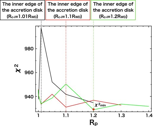
We start our analysis by applying our reflection model spectra to the outburst spectra. To begin, we have fixed Rc–i at 1.01, 1.1, 1.2. We believe these are reasonable as initial values of the inner edge of the AD based on previous works (<1.15 for HT Cas, Mukai et al. 1997; <1.12 for SS Cyg, Ishida et al. 2009). The plasma torus distance from the disk plane Dv is fixed at 0.0001 (≪1). This implies that the weighted mean of the hot plasma emission measure is located in the AD plane. With these two parameters fixed, we tried to evaluate the remaining parameter Rp using the method described in sub-subsection 3.2.1. The simulation results are shown in figure 6. The best fit is obtained at Rp = Rc–i = 1.01. This result suggests that the weighted center of the plasma emission is located close to the inner edge of the AD.
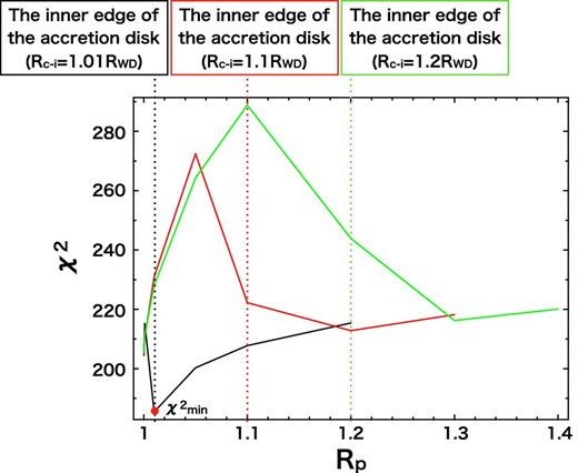
Best-fit χ2 values of the outburst spectra as a function of Rp, where Dv is fixed at 0.0001 (Dv ≪ 1). The black, red, and green lines indicate χ2 values when we assume Rc–i = 1.01, 1.1, and 1.2, respectively. (Color online)
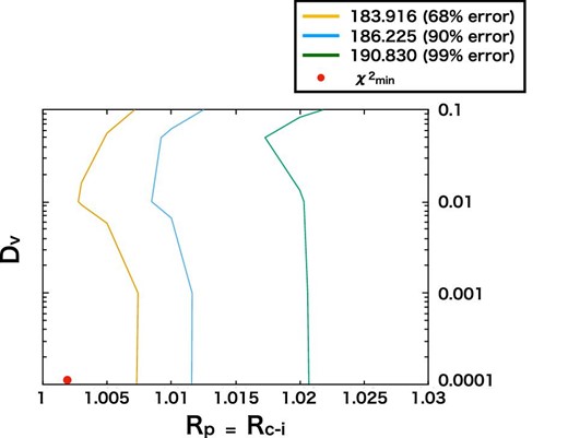
Second, we attempted to evaluate Rc–i and Rp by setting these two parameters free to vary but constrained to be the same (Rc–i = Rp). Figure 7 shows a χ2 contour map in the plane of Dv versus Rc–i (= Rp). The observed spectra are insensitive to Dv, and the best fit is obtained in the configuration where the inner edge of the AD reaches the surface of the WD. The two-parameter 90% upper limit is obtained to be Rc–i < 1.012. Note that this is an unexpected result based on the discussion in subsection 3.1. We will discuss this point later in subsection 4.2.
χ2 contour map in the plane of Dv versus Rc–i = Rp with the outburst spectra. The yellow, blue, and green lines indicate 68%, 90%, and 99% error, respectively. (Color online)
Finally, we attempted to determine whether the weighted center of the plasma Rp is still equal to Rc–i. In doing this, we fixed Dv and Rc–i at their best-fitting values of 0.0001 and 1.002, respectively. The results are shown in figure 8. We found that the result Rc–i = Rp is robust.
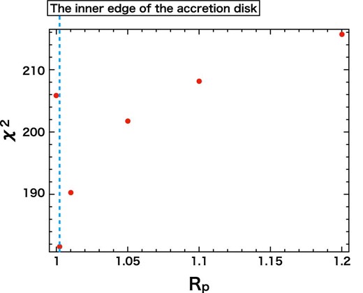
Variation of the χ2 value by altering Rp for the outburst spectra, where Dv and Rc–i are fixed at 0.0001 and 1.002, respectively. (Color online)
3.2.3 Evaluation of the quiescence spectra with the simulation spectrum model
We follow the same procedure on the quiescence spectra as for the outburst spectra. We begin with Dv fixed at 0.0001 (Dv ≪ 1) and Rc–i at 1.01, 1.1, 1.2 to find the best-fitting value of Rp. The results are shown in figure 9. This suggests that Rc–i = Rp, the same as in the case of the outburst.
Best-fit χ2 values of the quiescence spectra as a function of Rp, where Dv is fixed at 0.0001 (Dv ≪ 1). The black, red, and green lines indicate χ2 values when we assume Rc–i = 1.01, 1.1, and 1.2, respectively. (Color online)
We then performed the simulations to find the best-fitting pair of Dv and Rc–i = Rp. The χ2 contour map between Dv and Rc–i = Rp is shown in figure 10. The result is remarkably different from that in the outburst state (figure 7), in that Rc–i now has a lower limit of 1.08, irrespective of the Dv value. This indicates that the optically thick AD is truncated before it reaches the WD surface. The best-fitting Rc–i is located at Rc–i = 1.25 with Dv = 0.05. The lower and upper limits of Rc–i at the two-parameter 90% confidence level are 1.08 and 1.45, respectively, in the range Dv < 0.1.
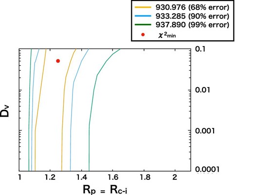
χ2 contour map in the plane of Dv versus Rc–i = Rp with the quiescence spectra. The yellow, blue, and green lines indicate 68%, 90%, and 99% error, respectively. (Color online)
Finally, we checked whether the relation Rp = Rc–i also holds in the quiescence state with Dv and Rc–i being fixed at their best-fitting values of 0.05 and 1.25, respectively (figure 10). The result is shown in figure 11. We obtained Rp = 1.25 as the best-fitting value, which is equal to Rc–i.
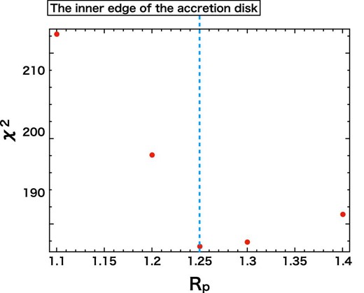
Variation of the χ2 value by altering Rp for the quiescence spectra, where Dv and Rc–i are fixed at 0.05 and 1.25, respectively. (Color online)
4 Discussion
4.1 Boundary layer geometry in quiescence
As shown in sub-subsection 3.2.3, we found that in quiescence the optically thick AD is truncated before it reaches the WD surface. The distance of the inner edge of the AD from the center of the WD is Rc–i = 1.25, with the 90% error of 1.08–1.45 in the range of Dv less than 0.1. This is in remarkable contrast to the case of several other DNe. For HT Cas, Mukai et al. (1997) obtained an upper limit of the size of the optically thin BL to be <1.15 based on the profile of the X-ray eclipse light curve. The other example is SS Cyg, for which Ishida et al. (2009) obtained an upper limit of <1.12 from the equivalent width of the 6.4 keV iron emission line. We obtained, on the other hand, a strong suggestion of disk truncation (the lower limit of the inner edge radius of the AD, Rc–i, being 1.08) from the X-ray observation for the first time. To reinforce this conclusion, we show the iron line spectrum of U Gem in quiescence, in comparison with that of SS Cyg, in figure 12. The narrow 6.4 keV iron emission line is detected from both U Gem (∼5 σ level, see figure 3) and SS Cyg, although it is significantly weaker for U Gem. As we mentioned earlier, the narrow 6.4 keV line is emitted from the WD surface via fluorescence. Therefore, this contrast in the two spectra indicates that the solid angle of the WD over the X-ray-emitting plasma is smaller in U Gem than that in SS Cyg, which is consistent with our reflection simulation result. Moreover, the abundance of iron is smaller in SS Cyg than U Gem (0.37|$^{+0.03}_{-0.01}\, Z_{\odot} $| versus 0.89 ± 0.05 Z⊙ in U Gem, see table 3). These two facts require that the X-ray-emitting hot plasma should be located farther from the WD in U Gem than in SS Cyg, which is consistent with our reflection simulation result in quiescence.
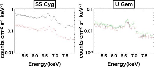
Comparison of the iron line spectra between SS Cyg and U Gem. The 6.4 keV line is weaker in U Gem. (Color online)
It was found by Rana et al. (2006), based on six nonmagnetic CV observations with the Chandra high-energy transmission grating, that the iron 6.4 keV lines show a significant variety in their nature. Their results also indicate that the 6.4 keV line is more prominent in SS Cyg than in U Gem. Such divergence probably originates from the difference in the disk-truncated radius demonstrated in our analysis above.
4.2 Boundary layer geometry in outburst
In sub-subsection 3.2.2, we showed that an optically thin BL could exist in U Gem in outburst between the WD surface and the inner edge of the AD, with an upper limit size of Rc–i < 1.012. However, it should be noted that, as shown in the contour map of figure 7, the best fit of Rc–i is ≃1.0, which favors the scenario that the outburst BL is optically thick, and the hard X-ray emission emanates from a site that is just above the AD, very close to the WD surface. From the spectral fit, such a configuration is more likely for U Gem in outburst, as in SS Cyg. In contrast, since we now have a reliable mass accretion rate that is smaller than the critical rate (subsection 3.1), thanks to the Gaia archive and the sophisticated spectral models, we believe the optically thin BL of U Gem in outburst is still a viable idea. One possible method to resolve this discrepancy is to introduce systematic uncertainty to the WD mass. If it is larger than the value used in this study, MWD = 1.07 M⊙ (Smak 2001), our reflection model could result in disk truncation and might be able to reproduce the broad 6.4 keV emission line as observed. Another possibility is calibration uncertainty of the line spread function and insufficient energy resolution of the XIS. As a matter of fact, the conclusion of Rc–i ≃ 1.0 is found to be unchanged when we increase the mass of the WD even up to 1.35 M⊙. This strongly suggests the insufficient energy resolution of the XIS to cope with this issue. Obviously, we should wait for the advent of a new-generation detector with a higher energy resolution, such as Resolve onboard the XRISM satellite, to provide the final conclusion on the disk truncation radius Rc–i.
4.3 The relation Rc–i = Rp
From our series of reflection simulations, we found that the radial plasma position Rp is equal to the radius of the inner edge of the AD Rc–i in both outburst and quiescence. Here, it should be noted that, in our simulation, the plasma torus width is zero, and hence Rp should be regarded as the weighted center of the differential emission measure of the plasma. Nevertheless, because the reflection is the source of the 6.4 keV iron emission line, which requires X-ray photons whose energy exceeds the iron K-edge energy 7.1 keV, the result Rp = Rc–i suggests that the plasma is heated up probably to the maximum temperature, or at least to a sufficiently high temperature to ionize a K-shell electron of Fe, e.g. >10 keV, by rapid deceleration and heating of the accreting matter immediately after it enters the BL. After that, the plasma gas is monotonically cooled as it approaches the WD through X-ray radiation. This picture is qualitatively in agreement with the fact that the X-ray spectrum of DNe in general can be fitted with the cooling flow model (Pandel et al. 2005; Baskill et al. 2005; Wada et al. 2017).
5 Summary
In this study we have presented our analysis of the Suzaku data for U Gem taken in 2012, both in quiescence and outburst, to understand the reason why, unlike SS Cyg, the hard X-ray flux increases in the optical outburst state. As a matter of fact, the X-ray intensity in outburst is greater than in quiescence in our data. Although the data span only one day, much shorter than the entire optical outburst cycle, our X-ray light curve in outburst seems to detect the peak of the outburst. If this identification is true, the X-ray outburst peak is retarded from the optical outburst peak by 2.1 d, with a conservative error of ±0.5 d.
It has been proposed that an optically thin BL emitting hard X-rays turns into an optically thick state emitting EUV emission when the mass transfer rate through the disk exceeds the critical rate of 1016 g s−1 (Pringle & Savonije 1979). Now that we have a reliable distance estimation provided by the Gaia archive and the accumulation of wisdom on the hard X-ray spectral model of the DNe, we have attempted to evaluate the mass accretion rate of U Gem through hard X-ray spectroscopy. Our analysis results in a mass accretion rate of |$\dot{M}=1.87\times 10^{14}$| g s−1 in outburst and |$\dot{M}=0.89\times 10^{14}$| g s−1 in quiescence. Because |$\dot{M}$| does not exceed the critical rate, the increase in the hard X-ray flux during the optical outburst state can be interpreted as the BL being kept in an optically thin state even in an outburst.
Although the mass accretion rates indicate similar BL geometry both in quiescence and outburst, the profiles of the 6.4 keV fluorescent Fe line are significantly different between the two states. Since the 6.4 keV Fe line reflects the geometry of the hard-X-ray-emitting plasma in relation to the WD surface and the AD, we attempted to simulate a reflection spectrum to elucidate the difference in plasma geometry between quiescence and outburst. A detailed spectral analysis with the model generated from the simulation clearly showed that, in quiescence, the optically thick AD is truncated at 1.25 RWD with a 90% error range of 1.08–1.45, and the optically thin hot plasma fills within this radius. Note that DNe disk truncation is indicated from the hard X-ray observation for the first time. Conversely, in outburst, our spectral analysis favors the notion that the optically thick disk, like SS Cyg, reaches the WD surface, although disk truncation can occur in the region <1.012 RWD. This apparent inconsistency with the optically thin BL geometry obtained from the mass accretion rate may be resolved if we are allowed to introduce a systematic error in the WD mass, or take into account possible calibration error of the line spread function and the insufficient energy resolution of the XIS. Obviously we need a new-generation detector with a higher energy resolution to provide the final conclusion to this issue.
Our spectral analysis also indicates that the optically thin thermal plasma is heated up to a temperature high enough to ionize a K-shell electron of iron (>10 keV) immediately after the accreting matter enters the BL. This is consistent with the fact that the hard X-ray spectra of the DNe can be explained by the cooling flow model in general.
The next Japanese X-ray astronomy satellite, X-Ray Imaging and Spectroscopy Mission (XRISM), to be launched in 2022 is known to be equipped with an X-ray microcalorimeter (Resolve) having an energy resolution approximately 30 times better than that of the CCD cameras that have been widely used as standard X-ray detectors. We will surely be able to achieve much finer spectroscopy, not only of the 6.4 keV line but also other emission lines, in order to understand the geometry and physical state of the hard X-ray-emitting plasma.
Footnotes
Mukai, K. 2009, poster presented at 5th Symp. Chandra’s First Decade of Discovery, Boston, MA, 2009 September 22–25.
References
