


Abstract
We make use of the ALMA twenty-Six Arcmin2 survey of GOODS-S At One-millimeter (ASAGAO), deep 1.2 mm continuum observations of a 26-arcmin2 region in the Great Observatories Origins Deep Survey-South (GOODS-S) obtained with Atacama Large Millimeter/sub-millimeter Array (ALMA), to probe dust-enshrouded star formation in K-band selected (i.e., stellar mass selected) galaxies, which are drawn from the FourStar Galaxy Evolution Survey (ZFOURGE) catalog. Based on the ASAGAO combined map, which was created by combining ASAGAO and ALMA archival data in the GOODS-South field, we find that 24 ZFOURGE sources have 1.2 mm counterparts with a signal-to-noise ratio >4.5 (1σ ≃ 30–70 μJy beam−1 at 1.2 mm). Their median redshift is estimated to be |$z$|median = 2.38 ± 0.14. They generally follow the tight relationship of the stellar mass versus star formation rate (i.e., the main sequence of star-forming galaxies). ALMA-detected ZFOURGE sources exhibit systematically larger infrared (IR) excess (IRX ≡ LIR/LUV) compared to ZFOURGE galaxies without ALMA detections even though they have similar redshifts, stellar masses, and star formation rates. This implies the consensus stellar-mass versus IRX relation, which is known to be tight among rest-frame-ultraviolet-selected galaxies, cannot fully predict the ALMA detectability of stellar-mass-selected galaxies. We find that ALMA-detected ZFOURGE sources are the main contributors to the cosmic IR star formation rate density at |$z$| = 2–3.
1 Introduction
Recent studies have revealed the evolution of the cosmic star formation rate density (SFRD) as a function of redshift based on various wavelengths (e.g., Madau & Dickinson 2014; Bouwens et al. 2015, 2016; and references therein). The roles of dust-obscured star-formation in star-forming galaxies at redshift |$z$| ≃ 1–3 and beyond are one of the central issues, because the majority of star-forming galaxies at |$z$| ≃ 1–3, where the cosmic star formation activity peaks, are dominated by dust-enshrouded star-formation.
At (sub-)millimeter wavelengths, several studies have found bright sub-millimeter galaxies (SMGs) whose observed flux densities are larger than a few mJy at (sub-)millimeter wavelengths (i.e., ∼850 μm–1 mm) in blank-field bolometer surveys (e.g., Smail et al. 1997; Barger et al. 1998; Hughes et al. 1998; Blain et al. 2002; Greve et al. 2004; Weiß et al. 2009; Scott et al. 2010; Hatsukade et al. 2011; Casey et al. 2013; Umehata et al. 2014, and references therein). The fact that (sub-)millimeter flux densities are almost constant at |$z$| > 1 for galaxies with a given infrared (IR) luminosity (i.e., the negative k-correction—e.g., Blain & Longair 1996) makes it efficient to study dust-obscured star-formation activity at high redshift and the extreme star-formation rates (SFRs) of SMGs [a few 100–1000 M⊙ yr−1, modulo expectations for and observations of the stellar initial mass function (IMF) in starburst environments—Papadopoulos et al. (2011), Zhang et al. (2018)] make them non-negligible contributors to the cosmic SFRD (e.g., Hughes et al. 1998; Wardlow et al. 2011; Casey et al. 2013; Swinbank et al. 2014).
Deep (sub-)millimeter-wave surveys, using the James Clerk Maxwell Telescope/Submillimeter Common-Use Bolometer Array 2 (SCUBA2; Holland et al. 2013), AzTEC (Wilson et al. 2008) on the Atacama Submillimeter Telescope Experiment (ASTE; Ezawa et al. 2004, 2008), LABOCA (Siringo et al. 2009) on the Atacama Pathfinder EXperiment (APEX; Güsten et al. 2006), Herschel/Spectral and Photometric Imaging Receiver (SPIRE; Griffin et al. 2010) and so on, play essential roles in revealing the contributions of dust-obscured star formation activities (e.g., Elbaz et al. 2011; Burgarella et al. 2013), but their limited angular resolution does not allow us to measure far-IR fluxes of individual sources if we go down to luminous IR galaxy (LIRG) class sources [i.e., IR luminosity (LIR) ∼ 1011 L⊙]. Indeed, the contribution of these “classical” SMGs (LIR ∼ 1012–1013 L⊙) to the integrated extragalactic background light is not so large (|${\sim}20\%$|–|$40\%$| at 850 μm and |$\sim 10\%$|–|$20\%$| at 1.1 mm; e.g., Eales et al. 1999; Coppin et al. 2006; Weiß et al. 2009; Hatsukade et al. 2011; Scott et al. 2012). This means that the bulk of dust-obscured star formation activities in the universe remained unresolved due to the confusion limit of single-dish telescopes.
Even with single-dish telescopes, we can access the fainter (sub-)millimeter population (i.e., observed flux densities Sobs ≲ 1 mJy) using gravitational magnification by lensing clusters or stacking analysis (e.g., Knudsen et al. 2008; Geach et al. 2013; Coppin et al. 2015). However, in lensed object surveys, the effective sensitivity comes at the cost of a reduced survey volume, which increases the cosmic variance uncertainty (e.g., Robertson et al. 2014).1 The stacking technique is a useful way to obtain the average properties of less-luminous populations, but individual source properties have remained unexplored. Therefore, more sensitive observations with higher angular resolution are needed.
The advent of the Atacama Large Millimeter/sub-millimeter Array (ALMA), which offers high sensitivity and angular resolution capabilities, has allowed the fainter (sub-)millimeter population to be revealed below the confusion limit of single-dish telescopes. For instance, the ALMA follow-up observation of the LABOCA Extended Chandra Deep Field South surveys (ALESS; e.g., Hodge et al. 2013; Swinbank et al. 2014; da Cunha et al. 2015) have yielded detections of faint submillimeter sources. Archival ALMA data has also been exploited to find many faint (sub-)millimeter sources (e.g., Hatsukade et al. 2013; Fujimoto et al. 2016; Oteo et al. 2016). ALMA has also been used to obtain “confusion-free”, deep contiguous maps in Subaru-XMM-Newton-Deep-Field (SXDF)-Ultra-Deep-Survey (UDS)-The Cosmic Assembly Near-infrared Deep Extragalactic Legacy Survey (CANDELS; ∼2 arcmin2, Tadaki et al. 2015; Hatsukade et al. 2016; Kohno et al. 2016; Wang et al. 2016) and (proto-)cluster fields including Hubble Frontier Fields (∼4 arcmin2 per cluster, e.g., González-López et al. 2017; Muñoz Arancibia et al. 2018) and Small Selected Area at 22h (SSA22; ∼6 to 20 arcmin2, Umehata et al. 2017, 2018). Tiered ALMA deep surveys with a “wedding-cake” approach have been conducted in the Hubble Ultra-Deep Field (HUDF; ∼1–4 arcmin2, Aravena et al. 2016; Rujopakarn et al. 2016; Walter et al. 2016; Dunlop et al. 2017; González-López et al. 2020) and the Great Observatories Origins Deep Survey-South field (GOODS-S; ∼26 arcmin2; Ueda et al. 2018; Hatsukade et al. 2018, and ∼69 arcmin2; Franco et al. 2018).
Faint (sub-)millimeter sources uncovered by these ALMA observations tend to preferentially have large stellar masses (≳1010 M⊙, Tadaki et al. 2015; Aravena et al. 2016; Bouwens et al. 2016; Dunlop et al. 2017). In fact, a tight correlation between the stellar masses and the infrared excesses, or IRXs, defined as a ratio of IR luminosity to ultraviolet (UV) luminosity (LIR/LUV), has been proposed (e.g., Bouwens et al. 2016; Fudamoto et al. 2017; Koprowski et al. 2018), mainly based on the ALMA fluxes of rest-frame-UV-selected galaxies such as Lyman break galaxies (LBGs). However, it is not entirely clear if the stellar mass is the unique parameter to predict IRXs in galaxies, and whether such a trend can be applicable to other types of galaxies such as rest-frame-optical-selected galaxies. It is also intriguing to see if there are low-mass galaxies with an elevated IRX or high-mass galaxies with a low IRX. Currently, the number of galaxies with both stellar-mass and IRX measurements using ALMA is still insufficient to address these questions.
Here, we present millimeter-wave properties of K-band selected galaxies in the FourStar galaxy evolution survey (ZFOURGE)2 catalog (Straatman et al. 2016) by exploiting the ALMA twenty-Six Arcmin2 survey of GOODS-S At One-millimeter (ASAGAO; Project ID: 2015.1.00098.S, PI: K. Kohno),3 one of the tiered ALMA deep surveys in HUDF/GOODS-S, to constrain dust-enshrouded star-forming properties of mass-selected galaxies and assess their contribution to the cosmic SFRD. The ZFOURGE catalog contains 30911 K-band selected galaxies over 128 arcmin2 in the Chandra Deep Field South, which fully includes the ASAGAO field, with a 5σ limiting AB magnitude of Ks = 26.0 to 26.3 at the |$80\%$| and |$50\%$| completeness levels (with masking), respectively. There are ≃ 3283 ZFOURGE sources within the ASAGAO field. Thanks to the high resolution of the ALMA mosaic image (≃|${^{\prime \prime}_{.}}5$|; see section 2 for details), we can select ALMA-detected K-band sources reliably to constrain their dusty star-formation properties.
This paper is structured as follows. Section 2 presents our ALMA observations and the source identifications. Then, we describe our strategy to obtain spectral energy distribution (SED) fits in section 3, and we discuss their derived physical properties in section 4. In section 5, we explain the contribution of K-band-detected ASAGAO sources to the cosmic SFRD. Section 6 presents our conclusions. Throughout this paper, we assume a Λ cold dark matter cosmology with ΩM = 0.3, ΩΛ = 0.7, and H0 = 70 km s−1 Mpc−1. All magnitudes are given according to the AB system. We adopt the Chabrier IMF (Chabrier 2003) in this paper.
2 ZFOURGE sources with ALMA counterparts
2.1 ALMA Band-6 data
In this paper, we use the ALMA data obtained by ASAGAO. As presented in Hatsukade et al. (2018), the 26 arcmin2 map of the ASAGAO field was obtained at 1.14 mm and 1.18 mm (two tunings) to cover a wider frequency range, whose central wavelength was 1.16 mm. In addition to the original ASAGAO data, we also included ALMA archival data of the same field (Project ID: 2015.1.00543.S, PI: D. Elbaz and Project ID: 2012.1.00173.S, PI: J. S. Dunlop) to improve the sensitivity. The data were imaged with the Common Astronomy Software Applications package (CASA; McMullin et al. 2007) version 5.1.1, but calibration was done with version 4.7.2. The maps were processed with the CLEAN algorithm (Högbom 1974) with the task tclean. Details of the data analysis are given in Hatsukade et al. (2018). The combined map reached typical rms noise of 30–70 μJy beam−1 with a synthesized beam of |${0{^{\prime \prime }_{.}}59} \times {0{^{\prime \prime }_{.}}53}$| (PA = −83°). Note that the typical sensitivity is calculated within the area covered by ASAGAO (i.e., the region enclosed by the yellow solid line shown in figure 1).
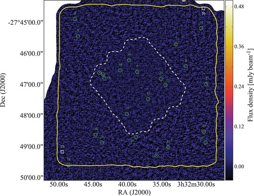
ASAGAO 1.2 mm continuum map of GOODS-S. ASAGAO original data, HUDF data (Dunlop et al. 2017), and a part of GOODS-ALMA data (Franco et al. 2018) are combined. In this paper, we only consider the ASAGAO field indicated by the yellow solid line (∼5′ × 5′). The white dashed line indicates the area covered by Dunlop et al. (2017). The green symbols indicate 24 ASAGAO continuum sources with K-band counterparts (see section 2.2). Two white squares show the positions of secure (S/N > 5.5) ASAGAO sources without ZFOURGE counterparts, which have been reported in a separate paper (Yamaguchi et al. 2019). (Color online)
2.2 ALMA counterparts identification
Since it has been reported that astrometric corrections are necessary for sources catalogued using HST and ZFOURGE images in GOODS-S (e.g., Rujopakarn et al. 2016; Dunlop et al. 2017; Franco et al. 2018), the ZFOURGE source coordinates were corrected by |$-{0{^{\prime \prime }_{.}}086}$| in right ascension and |$+{0{^{\prime \prime }_{.}}282}$| in declination, which is calibrated by the positions of stars in the Gaia Data Release 1 catalog (Gaia Collaboration 2016) within the ASAGAO field. We then measure ALMA flux densities of ZFOURGE sources. Although Bouwens et al. (2016) consider a S/N threshold of 2.0 to search for ALMA counterparts of LBGs, we adopt a more conservative threshold of S/N = 4.5. We extracted 45 positive sources and nine negative sources (i.e., false detections) with S/N > 4.5. Therefore, the ratio between the number of negative sources and positive sources is 0.2.
For point-like ZFOURGE sources, we allow the positional offsets between ZFOURGE and ALMA positions of less than |${0{^{\prime \prime }_{.}}5}$|, which is comparable with the synthesized beam of the combined ALMA map. Considering the number of ZFOURGE sources within the ASAGAO field (∼ 3000), the likelihood of random coincidence is estimated to be 0.03 (this likelihood is often called the p-value; Downes et al. 1986). In the case that a counterpart is largely extended, we allow a larger positional offset, up to the half-light radius of Ks-band emission. We exclude ZFOURGE sources with “use flag =0” (e.g., sources with low S/N at K-band or catastrophic SED fits; see Straatman et al. 2016 for details) in order to prevent mismatching. When we apply the same procedure to the negative values of the ALMA map, we find that no negative sources with an S/N ≲ −4.5 show chance coincidence. This coincidence rate is comparable with the estimated value by Casey et al. (2018).
Flux measurements in the ALMA map were performed at the position of ZFOURGE sources considering positional offset as explained above. We consider the flux-boosting effect by calculating the ratio between input and output integrated flux densities of 30000 artificial sources inserted into the signal map (see Hatsukade et al. 2018, for details). The effect of flux boosting for the sources with S/N > 4.5 is |$\lesssim 15\%$| (Hatsukade et al. 2018), which is comparable with previous studies.
Finally, we identify 24 ZFOURGE sources that have ALMA counterparts (hereafter, we define them as ASAGAO sources). Note that two ALMA sources without ZFOURGE source associations, or “NIR-dark ALMA sources”, have been reported in a separate paper (Yamaguchi et al. 2019). In table 1, we summarize ALMA fluxes of ZFOURGE sources in order of ALMA peak S/N. As shown in table 1, some ASAGAO sources show larger p-values than the traditional threshold of p < 0.05 (e.g., Biggs et al. 2011; Casey et al. 2013). We remove these ASAGAO sources with p > 0.05 (i.e., ID1 and ID7) from our conclusions presented in section 4 and section 5 to prevent mis-identifications. We show the positions of ASAGAO sources and their multi-wavelength postage stamps in figure 1 and figure 2, respectively.


Multi-wavelength images of ASAGAO sources with K-band counterparts. From left to right: ALMA 1.2 mm, JVLA 6 GHz (C band), Spitzer IRAC/4.5 μm, IRAC/3.6 μm, VLT HAWK-I/Ks, and HST WFC3/F160W images. The field of view is 5″ × 5″. Blue and magenta crosses mark the ALMA positions and ZFOURGE positions, respectively. Cyan circles are 1″ apertures. The synthesized beams of ALMA and JVLA are expressed as filled ellipses. ZFOURGE source IDs are shown in the HST/F160W images (in magenta).
ZFOURGE sources with ALMA counterparts.*
| ID | RAZFOURGE† | DecZFOURGE† | ID | S ALMA | S/Npeak | RAALMA | DecALMA | |Δoffset| | p-value | |$z$| photo | |$z$| spec | Chandra |
|---|---|---|---|---|---|---|---|---|---|---|---|---|
| (ZFOURGE) | (°) | (°) | (ASAGAO) | (mJy) | (°) | (°) | (″) | counterpart? | ||||
| (1) | (2) | (3) | (4) | (5) | (6) | (7) | (8) | (9) | (10) | (11) | (12) | (13) |
| 18658 | 53.18341 | −27.77646 | 1 | 0.985 ± 0.036 | 25.995 | 53.18348 | −27.77666 | 0.735 | 0.0578 | 2.83|$^{+0.07}_{-0.08}$| | — | Y |
| 17856 | 53.11880 | −27.78289 | 2 | 1.973 ± 0.075 | 25.625 | 53.11881 | −27.78288 | 0.048 | 0.0003 | 2.38|$^{+0.17}_{-0.10}$| | — | Y |
| 13086 | 53.14885 | −27.82119 | 3 | 1.748 ± 0.070 | 24.008 | 53.14885 | −27.82119 | 0.021 | 0.0 | 2.58|$^{+0.04}_{-0.04}$| | 2.582 | Y |
| 18645 | 53.18137 | −27.77756 | 4 | 0.906 ± 0.041 | 21.045 | 53.18137 | −27.77757 | 0.044 | 0.0002 | 2.92|$^{+0.06}_{-0.06}$| | — | |
| 18701 | 53.16061 | −27.77622 | 5 | 0.735 ± 0.039 | 18.101 | 53.16063 | −27.77628 | 0.228 | 0.0057 | 2.61|$^{+0.07}_{-0.05}$| | 2.543‡ | Y |
| 22177 | 53.19835 | −27.74788 | 6 | 0.922 ± 0.074 | 12.421 | 53.19830 | −27.74790 | 0.153 | 0.0026 | 1.93|$^{+0.04}_{-0.03}$| | — | Y |
| 20298 | 53.13735 | −27.76163 | 7 | 0.778 ± 0.086 | 8.785 | 53.13710 | −27.76141 | 1.124 | 0.13 | 0.52|$^{+0.02}_{-0.01}$| | 0.523 | |
| 19033 | 53.13112 | −27.77319 | 8 | 0.610 ± 0.072 | 8.654 | 53.13115 | −27.77320 | 0.084 | 0.0008 | 2.22|$^{+0.03}_{-0.03}$| | 2.225 | Y |
| 21234 | 53.19656 | −27.75704 | 9 | 0.457 ± 0.055 | 8.575 | 53.19656 | −27.75708 | 0.123 | 0.0017 | 2.46|$^{+0.05}_{-0.05}$| | — | |
| 18912 | 53.17092 | −27.77547 | 10 | 0.261 ± 0.031 | 8.550 | 53.17091 | −27.77544 | 0.099 | 0.0011 | 2.36|$^{+0.10}_{-0.11}$| | — | |
| 21730 | 53.12185 | −27.75278 | 11 | 0.635 ± 0.078 | 8.506 | 53.12186 | −27.75277 | 0.071 | 0.0006 | 2.01|$^{+0.06}_{-0.04}$| | — | Y |
| 16952 | 53.15405 | −27.79093 | 12 | 0.376 ± 0.049 | 7.378 | 53.15401 | −27.79087 | 0.251 | 0.0069 | 1.88|$^{+0.04}_{-0.03}$| | 1.317‡ | |
| 17733 | 53.14349 | −27.78328 | 13 | 0.400 ± 0.053 | 7.227 | 53.14351 | −27.78329 | 0.05 | 0.0003 | 1.62|$^{+0.04}_{-0.05}$| | 1.415‡ | |
| 18336 | 53.18053 | −27.77972 | 14 | 0.238 ± 0.035 | 7.178 | 53.18053 | −27.77971 | 0.038 | 0.0002 | 2.67|$^{+0.11}_{-0.15}$| | — | Y |
| 15702 | 53.16692 | −27.79882 | 15 | 0.416 ± 0.064 | 6.637 | 53.16694 | −27.79881 | 0.082 | 0.0007 | 1.93|$^{+0.03}_{-0.03}$| | 1.998 | Y |
| 19487 | 53.16558 | −27.76987 | 16 | 0.488 ± 0.065 | 6.491 | 53.16562 | −27.76991 | 0.194 | 0.0041 | 1.61|$^{+0.08}_{-0.06}$| | 1.551‡ | Y |
| 12438 | 53.20235 | −27.82627 | 18 | 0.975 ± 0.172 | 5.803 | 53.20236 | −27.82629 | 0.063 | 0.0004 | 1.07|$^{+0.03}_{-0.03}$| | — | Y |
| 14580 | 53.18585 | −27.81004 | 19 | 0.387 ± 0.073 | 5.659 | 53.18585 | −27.81004 | 0.024 | 0.0001 | 2.81|$^{+0.10}_{-0.10}$| | 2.593 | Y |
| 18270 | 53.14617 | −27.77995 | 23 | 0.182 ± 0.037 | 5.360 | 53.14620 | −27.77995 | 0.096 | 0.001 | 2.61|$^{+0.05}_{-0.06}$| | — | Y |
| 14146 | 53.18201 | −27.81420 | 26 | 0.222 ± 0.052 | 4.923 | 53.18198 | −27.81420 | 0.107 | 0.0013 | 2.41|$^{+0.18}_{-0.14}$|§ | — | Y |
| 14419 | 53.16144 | −27.81116 | 29 | 0.197 ± 0.046 | 4.835 | 53.16141 | −27.81114 | 0.115 | 0.0015 | 2.77|$^{+0.11}_{-0.10}$| | — | Y |
| 13714 | 53.14167 | −27.81665 | 31 | 0.733 ± 0.158 | 4.714 | 53.14175 | −27.81670 | 0.328 | 0.0118 | 2.53|$^{+0.09}_{-0.10}$| | — | Y |
| 14122 | 53.11914 | −27.81402 | 33 | 0.318 ± 0.079 | 4.701 | 53.11911 | −27.81405 | 0.136 | 0.002 | 3.32|$^{+0.44}_{-0.45}$| | — | |
| 14700 | 53.12011 | −27.80834 | 44 | 1.768 ± 0.447 | 4.546 | 53.12018 | −27.80825 | 0.401 | 0.0175 | 1.83|$^{+0.05}_{-0.05}$| | — |
*ZFOURGE sources with ALMA counterparts in order of ALMA S/N. Columns: (1) ZFOURGE ID. (2) and (3) ZFOURGE position. (4) ASAGAO ID. (5) Spatially integrated ALMA flux density (de-boosted). (6) ALMA peak S/N. (7) and (8) ASAGAO position. (9) The positional offset between ALMA and ZFOURGE. (10) The p-Values for each ASAGAO source. (11) The photometric redshift. (12) The spectroscopic redshift. (13) Based on cross-matching with the Chandra catalog (Luo et al. 2017); “Y” is assigned if the angular separation between the ALMA and Chandra sources is less than three times their combined 1σ positional error (see also Ueda et al. 2018).
†The systematic coordinate offsets have been corrected.
‡The spectroscopic redshift presented by Inami et al. (2017) using MUSE.
§The photometric redshift presented by Luo et al. (2017).
Ueda et al. (2018) and Fujimoto et al. (2018) also use ASAGAO data. In the tables of appendix 1, we present the correspondence of their ID to the ASAGAO ID, which is presented in this paper. We also cross-matched the ASAGAO sources with 1.3 mm sources of HUDF (Dunlop et al. 2017), 1.1 mm sources of GOODS-ALMA (Franco et al. 2018), 1.2 mm sources of ASPECS (Aravena et al. 2016), and 870 μm sources obtained by Cowie et al. (2018). The results of cross-matching are presented in table 3 in appendix 1.
2.3 Observed flux densities at 1.2 mm
In figure 3, we plot the histogram of observed flux densities of ASAGAO sources at 1.2 mm. As a comparison, we also show the histograms of observed flux densities obtained by ALESS (Hodge et al. 2013; da Cunha et al. 2015), HUDF (Dunlop et al. 2017), GOODS-ALMA (Franco et al. 2018), and ASPECS (Aravena et al. 2016). Note that ALESS sources, HUDF sources, and GOODS-ALMA sources were observed at 870 μm, 1.3 mm, and 1.1 mm, respectively. Therefore, we converted these flux densities to 1.2 mm flux densities with the assumption of a modified blackbody with a dust emissivity index of 1.5 and dust temperature of 35 K.4

Figure 3 shows that ASAGAO sources tend to have fainter flux densities (S1.2 mm ≲ 1 mJy) than most of the ALESS sources (S1.2 mm ≳ 1 mJy). Although recent ALMA contiguous surveys focusing on stellar-mass-selected sources (e.g., Aravena et al. 2016; Dunlop et al. 2017; Franco et al. 2018) also suggest that their samples tend to have flux densities of S1.2 mm ≲ 1 mJy, we provide the largest number of stellar-mass-selected sources with 1.2 mm flux densities.
2.4 Redshift distribution of ASAGAO sources
Straatman et al. (2016) estimate photometric redshifts of the ZFOURGE sources using the optical-to-near-IR SED fitting code EAZY (Brammer et al. 2008). Their SED fitting is based on 40 photometric points from U-band to Spitzer 8 μm band including the six FourStar medium-band filters (J1, J2, J3, Hs, Hl, and Ks band; see tables 1 and 2 of Straatman et al. 2016, for details). Some ZFOURGE sources have spectroscopic redshifts presented by Skelton et al. (2014). One of the ASAGAO sources, ASAGAO ID26, has an extremely large photometric redshift (|$z$| = 9.354), which is apparently caused by an incorrect SED fitting. On the other hand, Luo et al. (2017) present its photometric redshift as |$z$| = 2.14 and this is the value we use.5 Some sources are also observed by Inami et al. (2017) with the Multi Unit Spectroscopic Explorer (MUSE; Bacon et al. 2010). We use the spectroscopic redshifts of Inami et al. (2017) for ASAGAO sources that are detected by MUSE.
As shown in table 1, some ASAGAO sources have X-ray counterparts obtained by the Chandra Deep Field-South survey (Luo et al. 2017). Therefore, some ASAGAO sources appear to have active galactic nuclei (AGNs). However, Cowley et al. (2016) suggest that photometric redshifts estimated by ZFOURGE are appropriate for AGNs because of the benefits of medium-band filters. We also have to note that EAZY adopts K-luminosity priors, but it does not affect our results significantly. We calculate absolute differences between estimated photometric redshifts with K-luminosity priors and without priors for ASAGAO sources without spectroscopic redshifts (i.e., 15 sources, see table 1). The median value of the absolute differences is only 0.03.
Figure 4 shows the redshift distribution of ASAGAO sources. As a comparison, we also plot the results of ALESS (da Cunha et al. 2015), ALMA-detected sources with rest-frame optical/near-IR counterparts obtained by HUDF (Dunlop et al. 2017), and ALMA-non-detected ZFOURGE sources within the ASAGAO field (Straatman et al. 2016). The median redshift of 24 ASAGAO sources is estimated to be |$z$|median = 2.39 ± 0.14.6 This value is lower than that of ALESS sources (|$z$|median = 2.83 ± 0.22; da Cunha et al. 2015), which are significantly brighter than ASAGAO sources, and rather similar to that of sources in Dunlop et al. (2017) [|$z$|median = 2.04 ± 0.29, although this is partly due to the fact that there are some overlaps between sources in ASAGAO and Dunlop et al. (2017)].
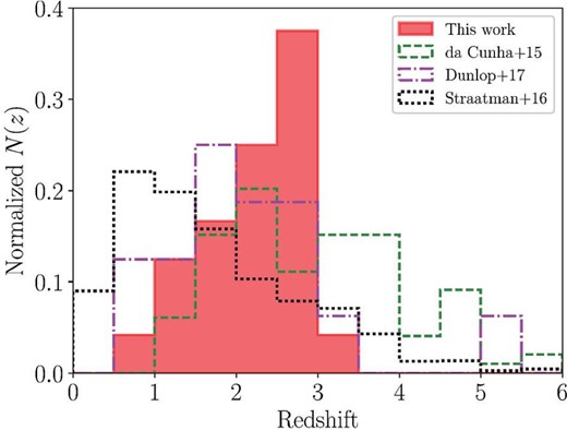
Normalized redshift distribution of the 24 ASAGAO sources with ZFOURGE counterparts (red-shaded region). The green dashed line, magenta dot–dashed line, and black dotted line indicate redshift distribution of ALESS sources (da Cunha et al. 2015), ALMA selected sources (Dunlop et al. 2017), and ZFOURGE sources within ASAGAO field (Straatman et al. 2016), respectively.
Many previous studies on “classical” SMGs (S1.2 mm ≳ a few mJy), including ALESS, report that median redshifts of “classical” SMGs are |$z$| ∼ 3, with a putative tail extending out to |$z$| ∼ 6 (e.g., Chapman et al. 2005; Simpson et al. 2014; da Cunha et al. 2015; Strandet et al. 2016). On the other hand, Aravena et al. (2016) suggest that their faint ALMA sources with optical/near-IR counterparts (S1.2 mm ∼ 50–500 μJy) reside in a lower redshift range than “classical” SMGs, although they only have small samples. The similar trend between photometric redshifts and ALMA 870 μm flux density for SCUBA2-selected SMGs in UDS is also reported by Stach et al. (2019). They find a significant trend of increasing redshift with increasing 870 μm flux density, which exhibits a gradient of dz/dS870 μm = 0.09 ± 0.02 mJy−1 (Stach et al. 2019). The redshift distribution of ASAGAO sources (S1.2 mm ≲ 1 mJy) is consistent with their results. Although we have to note that the difference of redshift distributions between (sub-)millimeter bright and faint sources can be caused by our sample selection (completenesses of optical/near-IR surveys drop significantly at high redshift), the difference is consistent with phenomenological models of Béthermin et al. (2015), which suggest that the median redshift of (sub-)millimeter sources declines with decreasing flux densities. According to Koprowski et al. (2017), the fact that lower-redshift sources tend to have lower (sub-)millimeter flux densities can be a direct consequence of the redshift evolution of the IR luminosity function (see also, e.g., Simpson et al. 2020).
3 SED fitting from optical to millimeter wavelengths
In order to investigate the properties of dusty star-formation among ASAGAO sources, we have to estimate dust-obscured SFRs. Therefore, we compiled photometries from mid-IR to millimeter wavelengths to estimate IR luminosities accurately. We include Spitzer/Multiband Imaging Photometer for the Spitzer (MIPS; Rieke et al. 2004; 24 μm), Herschel/Photodetector Array Camera and Spectrometer (PACS; Poglitsch et al. 2010; 100 and 160 μm), and Herschel/SPIRE (250, 350, and 500 μm) photometries, in addition to ZFOURGE data. Spitzer/MIPS 24 μm images are taken by Dickinson and FIDEL Team (2007) and the 1σ is 3.9 μJy (Straatman et al. 2016). Herschel/PACS images are taken by Magnelli et al. 2013 and their 1σ values are 205 and 354 μJy at 100 and 160 μm, respectively (Straatman et al. 2016).
For Herschel/SPIRE bands, we estimate de-blended flux densities by adopting the de-blending technique that has been described in detail in Liu et al. (2018). Here we have used all 24 μm and radio continuum sources as priors to extract fluxes in Herschel bands. From short to long wavelengths, after extracting source fluxes in shorter wavelength, we updated the flux prediction at longer wavelengths. With this predicted flux, we updated the prior list for extraction at longer wavelengths. For sources with predicted fluxes below the detection depth (typically two–three times the instrumental noise), we have frozen their fluxes to be the best predicted flux during the source extraction at longer wavelength, to reduce their effect on the source extraction for bright sources. In the end, we only count extracted flux for sources that are not frozen as real measurements. We then run Monte Carlo simulations by injecting sources into real maps and re-do the source extraction together with true priors to estimate the accuracy for flux and flux uncertainties. The typical flux uncertainties of de-blended SPIRE fluxes are estimated to be 2 to 3 mJy, which are similar to those in Liu et al. (2018). The details of the de-blending procedure in the ASAGAO field will be presented in T. Wang et al. (in preparation).
In this study, we perform Bayesian-based SED fitting from optical to millimeter wavelengths using MAGPHYS (see da Cunha et al. 2008, 2015 for details) to estimate the physical properties of the ASAGAO sources. We adopt the SED templates of Bruzual and Charlot (2003) and the dust extinction model of Charlot and Fall (2000). In the SED fitting, we fixed the redshift of the ASAGAO sources to the best-fitting photometric redshift presented by Straatman et al. (2016) or spectroscopic redshift if available (see table 1). Even if we consider the redshift uncertainties, our conclusions do not change significantly. For example, the changes in the estimated physical parameters are within ≲ 0.3 dex. Although we consider photometry errors in each band, we do not consider systematic uncertainties (e.g., absolute flux calibration errors), which does not affect our SED fitting results significantly.7 For ASAGAO sources, we use the MAGPHYS high-|$z$| extension version. This code uses priors which are optimized for IR luminous dusty star-forming galaxies at high redshift (da Cunha et al. 2015).
We have to note that MAGPHYS ignores any contribution by an AGN. Although Hainline et al. (2011) suggest that the near-IR continuum excess can be caused by the AGNs, only |$11\%$| of their sample (≃ 70 bright SMGs from Chapman et al. 2005) show stronger AGN-contribution than stellar-contribution at near-IR wavelengths. They also suggest that nearly half of their sample has less than |$10\%$| AGN-contribution to the near-IR emissions (the median value seems to be |$\sim 10\%$|–|$20\%$|, according to figure 6 of Hainline et al. 2011). Dunlop et al. (2017) suggest that an AGN component in faint (sub-)millimeter sources would contribute only |$\simeq 20\%$| to the IR luminosity and near identical values are obtained by simply fitting the star-forming component to the ALMA data points. Michałowski et al. (2014) also suggest that the contribution of the AGNs does not have any significant impact on the derived stellar masses of (sub-)millimeter sources, although some bright SMGs contain very luminous AGNs (e.g., Ivison et al. 1998) and the near-ubiquity of accreting black holes in SMGs are reported (e.g., Alexander et al. 2005). In the case of ASAGAO-detected sources, Ueda et al. (2018) suggest that majority of X-ray detected ASAGAO sources appear to be star-formation-dominant populations. Based on these considerations, in the following analysis we assume that the contribution from an AGNs (if any) will have negligible impact on the physical properties derived from the SED analysis.
The results of SED fitting are shown in table 2 and figure 5. In table 2, we add a flag to distinguish whether a source has a good (flag = 1) or unreliable fit (flag = 0). We manually remove four sources with flag = 0 from the following discussion.8


Estimated SEDs of ASAGAO sources. Red symbols with errors are observed flux densities. Blue solid lines are the best-fitting SEDs estimated by MAGPHYS (see section 3). The black dashed lines are the best-fitting SEDs using a modified blackbody + mid-IR power-law model by Casey (2012). (Color online)
Results of the SED fitting.*
| ID | ID | log (M*) | log (M*) | log (LIR) | log (LIR) | log (LUV) | |$\log (\mathit {SFR}_\mathrm{UV+IR})$| | |$\log (\mathit {SFR}_\mathrm{UV+IR})$| | βUV | flag |
|---|---|---|---|---|---|---|---|---|---|---|
| (ZFOURGE) | (ASAGAO) | (ZFOURGE) | (MAGPHYS) | (MAGPHYS) | (Casey 2012) | (MAGPHYS) | (ZFOURGE) | (MAGPHYS) | ||
| [M⊙] | [M⊙] | [L⊙] | [L⊙] | [L⊙] | [M⊙ yr−1] | [M⊙ yr−1] | ||||
| (1) | (2) | (3) | (4) | (5) | (6) | (7) | (8) | (9) | (10) | (11) |
| 18658 | 1 | 10.11|$^{+0.00}_{-0.09}$| | 10.91|$^{+0.00}_{-0.00}$| | 12.74|$^{+0.00}_{-0.00}$| | — | 10.26|$^{+0.04}_{-0.04}$| | 2.62|$^{+0.01}_{-0.01}$| | 2.78|$^{+0.00}_{-0.00}$| | −1.53 ± 0.07 | 0 |
| 17856 | 2 | 10.84|$^{+0.11}_{-0.05}$| | 11.43|$^{+0.00}_{-0.00}$| | 12.75|$^{+0.00}_{-0.00}$| | 12.82 ± 0.02 | 9.63|$^{+0.06}_{-0.07}$| | 2.39|$^{+0.01}_{-0.01}$| | 2.79|$^{+0.00}_{-0.00}$| | 0.14 ± 0.27 | 1 |
| 13086 | 3 | 11.09|$^{+0.00}_{-0.01}$| | 11.70|$^{+0.00}_{-0.00}$| | 12.83|$^{+0.00}_{-0.00}$| | 12.81 ± 0.02 | 9.97|$^{+0.05}_{-0.06}$| | 3.11|$^{+0.00}_{-0.00}$| | 2.87|$^{+0.00}_{-0.00}$| | −0.43 ± 0.16 | 1 |
| 18645 | 4 | 10.78|$^{+0.22}_{-0.21}$| | 11.59|$^{+0.00}_{-0.01}$| | 12.43|$^{+0.00}_{-0.00}$| | 12.34 ± 0.03 | 8.94|$^{+0.19}_{-0.36}$| | 2.47|$^{+0.02}_{-0.02}$| | 2.46|$^{+0.00}_{-0.00}$| | — | 1 |
| 18701 | 5 | 10.48|$^{+0.00}_{-0.57}$| | 10.68|$^{+0.00}_{-0.00}$| | 12.51|$^{+0.00}_{-0.00}$| | 12.66 ± 0.03 | 10.08|$^{+0.03}_{-0.04}$| | 2.67|$^{+0.01}_{-0.01}$| | 2.55|$^{+0.00}_{-0.00}$| | −1.45 ± 0.14 | 1 |
| 22177 | 6 | 10.71|$^{+0.09}_{-0.03}$| | 11.37|$^{+0.19}_{-0.03}$| | 12.57|$^{+0.03}_{-0.00}$| | 12.60 ± 0.03 | 9.69|$^{+0.06}_{-0.07}$| | 2.43|$^{+0.01}_{-0.01}$| | 2.61|$^{+0.03}_{-0.00}$| | −0.51 ± 0.18 | 1 |
| 20298 | 7 | 10.27|$^{+0.09}_{-0.02}$| | 10.92|$^{+0.08}_{-0.00}$| | 11.00|$^{+0.00}_{-0.04}$| | — | 8.87|$^{+0.22}_{-0.47}$| | 1.04|$^{+0.02}_{-0.01}$| | 1.04|$^{+0.01}_{-0.05}$| | — | 0 |
| 19033 | 8 | 11.16|$^{+0.07}_{-0.09}$| | 11.66|$^{+0.00}_{-0.00}$| | 12.41|$^{+0.00}_{-0.00}$| | 12.34 ± 0.05 | 10.36|$^{+0.05}_{-0.06}$| | 2.61|$^{+0.01}_{-0.00}$| | 2.46|$^{+0.00}_{-0.00}$| | −0.43 ± 0.09 | 1 |
| 21234 | 9 | 9.97|$^{+0.08}_{-0.76}$| | 10.19|$^{+0.00}_{-0.00}$| | 11.78|$^{+0.00}_{-0.00}$| | 11.72 ± 0.09 | 9.03|$^{+0.13}_{-0.20}$| | 1.47|$^{+0.09}_{-0.08}$| | 1.82|$^{+0.00}_{-0.00}$| | −0.61 ± 0.80 | 1 |
| 18912 | 10 | 10.51|$^{+0.12}_{-0.08}$| | 11.09|$^{+0.04}_{-0.02}$| | 11.91|$^{+0.01}_{-0.02}$| | 11.89 ± 0.07 | 8.94|$^{+0.17}_{-0.27}$| | 2.01|$^{+0.03}_{-0.02}$| | 1.95|$^{+0.01}_{-0.02}$| | — | 1 |
| 21730 | 11 | 10.54|$^{+0.01}_{-0.08}$| | 11.40|$^{+0.00}_{-0.00}$| | 12.11|$^{+0.00}_{-0.00}$| | 12.08 ± 0.07 | 8.77|$^{+0.27}_{-0.85}$| | 2.14|$^{+0.02}_{-0.01}$| | 2.14|$^{+0.00}_{-0.00}$| | — | 1 |
| 16952 | 12 | 10.41|$^{+0.05}_{-0.06}$| | 11.12|$^{+0.00}_{-0.00}$| | 11.90|$^{+0.00}_{-0.00}$| | 11.82 ± 0.08 | 9.42|$^{+0.08}_{-0.10}$| | 2.08|$^{+0.02}_{-0.01}$| | 1.94|$^{+0.00}_{-0.00}$| | −0.59 ± 0.37 | 1 |
| 17733 | 13 | 10.79|$^{+0.00}_{-0.05}$| | 11.57|$^{+0.05}_{-0.00}$| | 12.04|$^{+0.03}_{-0.00}$| | 12.00 ± 0.04 | 9.08|$^{+0.23}_{-0.50}$| | 2.02|$^{+0.02}_{-0.01}$| | 2.08|$^{+0.03}_{-0.00}$| | −2.03 ± 0.02 | 1 |
| 18336 | 14 | 10.44|$^{+0.14}_{-0.07}$| | 11.10|$^{+0.04}_{-0.06}$| | 12.12|$^{+0.08}_{-0.07}$| | 12.10 ± 0.10 | 9.27|$^{+0.09}_{-0.11}$| | 1.22|$^{+0.20}_{-0.31}$| | 2.16|$^{+0.08}_{-0.07}$| | — | 1 |
| 15702 | 15 | 10.63|$^{+0.13}_{-0.08}$| | 11.38|$^{+0.00}_{-0.00}$| | 12.32|$^{+0.00}_{-0.00}$| | 12.36 ± 0.04 | 10.21|$^{+0.06}_{-0.07}$| | 2.58|$^{+0.01}_{-0.00}$| | 2.37|$^{+0.00}_{-0.00}$| | −1.38 ± 0.19 | 1 |
| 19487 | 16 | 11.24|$^{+0.00}_{-0.07}$| | 11.61|$^{+0.00}_{-0.00}$| | 11.98|$^{+0.00}_{-0.00}$| | 11.93 ± 0.06 | 9.45|$^{+0.18}_{-0.30}$| | 2.29|$^{+0.01}_{-0.01}$| | 2.02|$^{+0.00}_{-0.00}$| | −0.05 ± 0.61 | 1 |
| 12438 | 18 | 10.48|$^{+0.18}_{-0.04}$| | 11.37|$^{+0.06}_{-0.07}$| | 11.93|$^{+0.02}_{-0.01}$| | — | 8.67|$^{+0.15}_{-0.23}$| | 1.56|$^{+0.02}_{-0.01}$| | 1.97|$^{+0.02}_{-0.01}$| | — | 0 |
| 14580 | 19 | 10.65|$^{+0.02}_{-0.04}$| | 10.97|$^{+0.00}_{-0.00}$| | 11.97|$^{+0.00}_{-0.00}$| | 11.72 ± 0.12 | 9.87|$^{+0.04}_{-0.05}$| | 2.05|$^{+0.03}_{-0.02}$| | 2.02|$^{+0.00}_{-0.00}$| | −0.69 ± 0.16 | 1 |
| 18270 | 23 | 10.71|$^{+0.03}_{-0.00}$| | 11.36|$^{+0.02}_{-0.12}$| | 11.90|$^{+0.09}_{-0.16}$| | 11.89 ± 0.12 | 9.38|$^{+0.08}_{-0.10}$| | 2.09|$^{+0.04}_{-0.03}$| | 1.94|$^{+0.09}_{-0.16}$| | −0.64 ± 0.60 | 1 |
| 14146 | 26 | 11.49|$^{+0.03}_{-0.00}$| | 11.14|$^{+0.18}_{-0.09}$| | 12.45|$^{+0.02}_{-0.01}$| | 12.46 ± 0.05 | 8.14|$^{+0.44}_{-0.11}$| | — | 2.49|$^{+0.02}_{-0.01}$| | — | 1 |
| 14419 | 29 | 10.80|$^{+0.08}_{-0.27}$| | 11.35|$^{+0.00}_{-0.05}$| | 12.07|$^{+0.00}_{-0.06}$| | 11.93 ± 0.13 | 8.92|$^{+0.29}_{-1.55}$| | 2.16|$^{+0.03}_{-0.03}$| | 2.11|$^{+0.00}_{-0.06}$| | −0.41 ± 0.65 | 1 |
| 13714 | 31 | 11.00|$^{+0.05}_{-0.12}$| | 11.48|$^{+0.02}_{-0.05}$| | 12.11|$^{+0.11}_{-0.04}$| | 11.80 ± 0.19 | 9.12|$^{+0.24}_{-0.59}$| | 2.18|$^{+0.02}_{-0.02}$| | 2.15|$^{+0.11}_{-0.04}$| | −1.07 ± 1.04 | 1 |
| 14122 | 33 | 10.33|$^{+0.17}_{-0.08}$| | 10.95|$^{+0.08}_{-0.09}$| | 11.95|$^{+0.24}_{-0.41}$| | — | 8.49|$^{+0.10}_{-0.13}$| | 1.67|$^{+0.23}_{-0.51}$| | 1.99|$^{+0.24}_{-0.41}$| | — | 0 |
| 14700 | 44 | 10.79|$^{+0.08}_{-0.08}$| | 11.79|$^{+0.00}_{-0.00}$| | 12.16|$^{+0.00}_{-0.00}$| | 12.29 ± 0.13 | 9.04|$^{+0.27}_{-0.82}$| | 2.54|$^{+0.01}_{-0.00}$| | 2.19|$^{+0.00}_{-0.00}$| | −1.94 ± 0.76 | 1 |
*Columns: (1) ZFOURGE ID. (2) ASAGAO ID. (3) Stellar mass values taken from the ZFOURGE catalog (Straatman et al. 2016), which are obtained using FAST. (4) Stellar mass obtained by MAGPHYS. (5) IR luminosity obtained by MAGPHYS. (6) IR luminosity obtained using Casey (2012) model. (7) UV luminosity obtained by rest-frame 2800 Å luminosity. (8) UV + IR SFR obtained by ZFOURGE (Straatman et al. 2016). (9) UV + IR SFR obtained by MAGPHYS. (10) UV spectral slope estimated by fitting a power law fλ ∝ λβ over the rest-frame wavelength range of 1500–2500 Å. (11) SED fitting flag (1: good, 0: bad). The reasons to classify as flag =0 are (a) the number of photometry points is less than 12 (i.e., the degree of freedom of SED fit using MAGPHYS is less than one), (b) the predicted millimeter photometry is inconsistent with the observed ALMA photometry and there are no photometry points at mid-IR-to-far-IR wavelengths, and (c) the p-value is larger than 0.05.
4 Physical properties
4.1 Stellar masses and SFRs
We estimate the IR luminosities by mid-IR to far-IR SED templates obtained by Casey (2012) to confirm reliability of IR luminosities estimated by MAGPHYS for sources with flag = 1 (table 2). Casey (2012) assume a modified blackbody radiation plus a mid-IR power-law SED. Here, we assume an emissivity index equals 1.6 and mid-IR slope of 1.5 as discussed in Casey (2012). As shown in table 2 and figure 6, there is no significant systematic offset between the two methods.
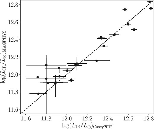
Comparison between IR luminosities estimated using the SED model by Casey (2012) and MAGPHYS. The black dashed line indicates the case that log (LIR/|$M_\odot$|)Casey2012 = log (LIR/|$M_\odot$|)MAGPHYS.
In table 2, we show the stellar masses and SFRs of ASAGAO sources obtained by Straatman et al. (2016). They used the FAST code (Kriek et al. 2009) to derive stellar masses. To estimate UV + IR SFRs, they used IR luminosities obtained by the IR SED template of Wuyts et al. (2008) in conjunction with MIPS 24 μm, PACS 100 μm, and PACS 160 μm photometries and UV luminosities from the rest-frame 2800-Å luminosity. We compare our results with the ZFOURGE to check consistency in figure 7. Although the SFRs estimated as with MAGPHYS and ZFOURGE are consistent, the stellar masses obtained by using MAGPHYS are systematically higher than that of FAST by ≳ 0.2–0.5 dex. A similar offset is also reported by Michałowski et al. (2014) and they suggest that it can be explained by the difference of the assumed star formation histories. de Barros Schaerer, and Stark (2014) suggest that nebular emission lines at near-IR wavelengths, which are not included in MAGPHYS, can lead to an overestimation of the stellar masses. Here, we use stellar masses obtained with FAST to compare our results with the ZFOURGE results (estimated by FAST) directly. In this paper, we compare the derived stellar masses of ASAGAO sources with stellar masses of other (sub-)millimeter selected samples obtained by previous studies. Therefore, we have to note the differences of stellar mass modeling. For example, Yamaguchi et al. (2016) also used FAST to estimate stellar masses. However, da Cunha et al. (2015) used MAGPHYS, and Dunlop et al. (2017) estimate stellar masses of ALMA sources by their SED fit using Bruzual and Charlot (2003) evolutionary synthesis models.

(Left) Comparison of stellar masses obtained by MAGPHYS and FAST. The black dashed line indicates the case that log (M*/|$M_\odot$|)MAGPHYS = log (M*/|$M_\odot$|)FAST. (Right) Comparison of IR + UV SFRs obtained by MAGPHYS and ZFOURGE. The black dashed line indicates the case that |$\log (\mathit {SFR}_\mathrm{UV+IR})_\mathrm{MAGPHYS} = \log (\mathit {SFR}_\mathrm{UV+IR})_\mathrm{ZFOURGE}$|.
Figure 8 shows the stellar mass distribution of ASAGAO sources. We only include ASAGAO sources with SED fitting flag = 1. Here, we divide ASAGAO sources into two redshift bins (i.e., 1.0 < |$z$| ≤ 2.0, and 2.0 < |$z$| ≤ 3.0). We have to note that ID7 and ID33 are both excluded here even if they lie at |$z$| < 1.0 and |$z$| > 3.0, respectively. In each redshift bin, there are seven and 15 ASAGAO sources, respectively. The median stellar masses of each redshift bin are log (M*/M⊙) = 10.75 ± 0.10 and 10.75 ± 0.11 for 1.0 < |$z$| ≤ 2.0, and 2.0 < |$z$| ≤ 3.0, respectively. The estimated stellar masses are consistent with previous studies on ALMA continuum sources at similar redshift range and with Sobs ≃ 1 mJy, such as Tadaki et al. (2015) or Dunlop et al. (2017). As shown in figure 8, the ASAGAO sources have typically higher stellar masses than ALMA-non-detected ZFOURGE sources, whose median stellar masses are log (M*/M⊙) = 8.96 ± 0.05 and 9.17 ± 0.04 for 1.0 < |$z$| ≤ 2.0 and 2.0 < |$z$| ≤ 3.0, respectively.10 This trend can be clearly observed when we plot the ALMA detection rate (i.e., ALMA-detected ZFOURGE sources per all ZFOURGE sources within the ASAGAO field) as a function of their stellar masses (figure 8). The trend is also shown in previous ALMA surveys such as Bouwens et al. (2016). Figure 8 shows the SFR distribution of ASAGAO sources in two redshift bins. The median SFR of each redshift bin is |$\log (\mathit {SFR}/[M_\odot \:\mbox{yr}^{-1}]) = 2.14 \pm 0.13$| and 2.15 ± 0.14 for 1.0 < |$z$| ≤ 2.0 and 2.0 < |$z$| ≤ 3.0, respectively.
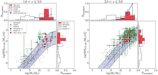
Comparison of the stellar masses and SFRs of ASAGAO sources with the “main sequence of star-forming galaxies”. ASAGAO sources are plotted as red circles. The gray crosses, green squares, orange triangles, black diamonds, and magenta inverted triangles represent the ALMA non-detected ZFOURGE sources (Straatman et al. 2016), ALESS sources (da Cunha et al. 2015), ASPECS sources (Aravena et al. 2016), faint SMGs from Yamaguchi et al. (2016), and ALMA selected sources from Dunlop et al. (2017). The blue solid lines indicate the position of the main sequence of star-forming galaxies at |$z$| = 1.83 (left) and 2.53 (right) as predicted by Schreiber et al. (2015). The blue dashed lines indicate a factor of 4 above or below this main sequence. In addition, we show the histograms of stellar masses and SFRs. The blue circles in the stellar-mass distributions are ALMA detection rates as a function of their stellar masses. The error bars show simple Poisson uncertainties. (Color online)
In figure 8, we plot the ASAGAO sources on the M*–SFR plane. In addition, we show the ALMA non-detected ZFOURGE sources within the ASAGAO field (Straatman et al. 2016), ALESS sources (da Cunha et al. 2015), ASPECS sources (Aravena et al. 2016), faint SMGs in SXDF-UDS-CANDELS (Yamaguchi et al. 2016), and ALMA sources with optical/near-IR counterparts by Dunlop et al. (2017). For comparison, we also plot the position of the main sequence of star-forming galaxies at each redshift (|$z$| = 1.83 and 2.53; median redshifts of each redshift bin) compiled by Schreiber et al. (2015).
As shown in figure 8, the ASAGAO sources primarily lie on the main sequence of star-forming galaxies, although some ASAGAO sources shows starburst-like features. Here we adopt the definition of a “starburst” mode from Schreiber et al. (2015), where an SFR increased by more than a factor of 4 (or 0.6 dex) compared to the main sequence. This is consistent with previous ALMA results (e.g., da Cunha et al. 2015; Aravena et al. 2016; Yamaguchi et al. 2016; Dunlop et al. 2017). Figure 8 also suggests that ASAGAO sources mainly trace the high-mass end of the main sequence of star-forming galaxies. When we compare ASAGAO sources with ALESS sources (i.e., single-dish-selected galaxies), ASAGAO sources tend to have systematically lower SFRs for a similar stellar mass range. Here we need to note that da Cunha et al. (2015) used MAGPHYS to estimate stellar masses of ALESS sources. When we consider the systematic offset of stellar masses estimated by MAGPHYS and FAST, differences between ASAGAO sources and ALESS sources on the M*–SFR plane become even larger. This result implies that an ALMA continuum survey at a 1σ depth of a few tens of μJy can unveil galaxies which are more likely the normal star-forming galaxies than “classical” SMGs since they show more quiescent star-forming activities than “classical” SMGs for a similar stellar mass range.
4.2 The infrared excess (IRX)
As shown in figure 8, there are ALMA-non-detected ZFOURGE sources within the ASAGAO field even though they show similar star-forming properties to ALMA-detected sources on the M*–SFR plane. In this section, we focus on IRX (i.e., LIR/LUV) as a key parameter to distinguish between ALMA-detected sources and non-detected sources. Although many previous studies on IRX of galaxies use rest-frame 1600 Å luminosities, we note that we adopt LUV = 1.5νLν2800 to obtain LUV (see subsection 4.1), which are supposed to be approximately equivalent (Kennicutt 1998; Whitaker et al. 2014).
4.2.1 The IRX–M* and IRX–SFR relations
Several studies have shown a correlation between the IRX and stellar masses, in the sense that massive star-forming galaxies show larger IRX (e.g., Reddy et al. 2010; Whitaker et al. 2014; Bouwens et al. 2016; Dunlop et al. 2017). We plot the IRX of ASAGAO sources as a function of their stellar masses in figure 9. For comparison, we also show the ALMA-detected sources (da Cunha et al. 2015; Dunlop et al. 2017) and ALMA-non-detected ZFOURGE sources (Straatman et al. 2016) within the ASAGAO field. We also show the consensus IRX–M* relation compiled by Bouwens et al. (2016). They derive stellar masses using FAST and their estimated consensus relationship is consistent with the results of three separate studies (Reddy et al. 2010; Whitaker et al. 2014; Álvarez-Márquez et al. 2016).
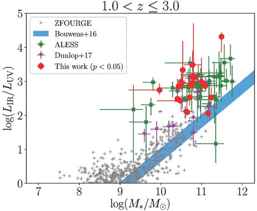
IRX of ASAGAO sources as a function of their stellar mass (red circles). We also show the ALMA-non-detected ZFOURGE sources (Straatman et al. 2016) within the ASAGAO field, ALESS sources (da Cunha et al. 2015), and ALMA-selected sources from Dunlop et al. (2017). The thick shaded blue line shows the consensus relation compiled by UV-selected galaxies at |$z$| ∼ 2–3 (Bouwens et al. 2016). (Color online)
As shown in figure 9, the ALMA-detected sources tend to have larger IRX compared to the ALMA-non-detected sources. The IRXs of ASAGAO sources at |$z$| > 1.0 are systematically larger than those from the IRX–M* relation of UV-selected galaxies, with an offset of 1–2 dex; in contrast, no ALMA-non-detected ZFOURGE sources exhibit such elevated IRX values. When we plot the IRX–SFR relation of ASAGAO sources for three stellar mass bins [i.e., log (M*/M⊙) ≤ 10, 10 < log (M*/M⊙) ≤ 11, and 11 < log (M*/M⊙); figure 10], the offset from ALMA-non-detected ZFOURGE sources also become evident.

4.2.2 The IRX–βUV relation
A useful relation to study the properties of dust is the relation between the UV spectral slopes (βUV) and IRX, because this relation reflects the effect of dust attenuation. Therefore, we examine the IRX–βUV relation of ALMA-detected sources for further discussion on the difference between ALMA-detected and -non-detected sources. The IRX–βUV relation has been calibrated using local star-burst galaxies (e.g., Meurer et al. 1999; Takeuchi et al. 2012).
In this study, βUV is calculated by fitting a power law fλ ∝ λβ over the rest-frame wavelength range of 1500–2500 Å using ZFOURGE photometies. Figure 11 shows the IRX–βUV relation of ASAGAO sources. We also plot the ALMA-non-detected ZFOURGE sources within the ASAGAO field, along with the relation given in Meurer et al. (1999) and Takeuchi et al. (2012). We find that ASAGAO sources tend to have larger IRX values compared to the ALMA-non-detected ZFOURGE sources, as well as the local starburst relations as provided by Meurer et al. (1999) and Takeuchi et al. (2012). This trend is consistent with the results in the COSMOS field by Casey et al. (2014), and a recent update by Fudamoto et al. (2020), although some ASAGAO sources exhibit more elevated IRX values. ALMA-bright LBGs at z = 3 − 6 in the UDS field (Koprowski et al. 2020) also exhibit similar trends in figure 11.

IRX of the ASAGAO sources as a function of βUV (red circles). Black crosses indicate ALMA-non-detected ZFOURGE sources (Straatman et al. 2016) within the ASAGAO field. The blue solid and dashed lines are the IRX–βUV relations of Meurer et al. (1999) and Takeuchi et al. (2012), respectively. (Color online)
Then why do dusty star-forming galaxies lie above the local IRX–βUV relations given by Meurer et al. (1999) and Takeuchi et al. (2012)? One of the possible drivers is the difference in a starburst time-scale (Casey et al. 2014). Dusty star-forming galaxies have short-timescale starburst (10–300 Myr), and short-lived burst events produce many young O and B stars that are not entirely enshrouded in thick dust cocoons yet. Another driver for the elevated IRX values is the dust composition (i.e., the difference of the chemical composition or/and the grain size distribution; e.g., Safarzadeh et al. 2017; Galliano et al. 2018). The geometry of dust and stellar components will also have significant impact on the IRX–βUV relation. In fact, starburst galaxies hosting heavily obscured regions together with a small fraction of non-obscured regions (e.g., “holes in dust shields”) can easily deviate from the local relation, because their UV and IR fluxes no longer come from the same region of a galaxy (e.g., Popping et al. 2017; Narayanan et al. 2018; Fudamoto et al. 2020). Significant difference between the dust-obscured star-forming regions and less-obscured rest-UV-emitting regions has been reported by recent ALMA observations (e.g., Hodge et al. 2015; Chen et al. 2017; Tadaki et al. 2017), and ASAGAO sources discussed here are also reported to exhibit such difference (Fujimoto et al. 2018). Detailed comparison with the (sub)millieter and rest-UV distributions of these sources with higher resolution observations will be useful to quantitatively address the impact of dust-stellar geometry on the measured IRX–βUV relations.
It has also been claimed that dust temperature (e.g., Faisst et al. 2017; Narayanan et al. 2018) and the presence of a low-level AGN (Saturni et al. 2018) can also affect IRX–βUV relations of dusty sources. Spatially resolved shorter-wave ALMA observations will be necessary to disentangle the impact of warm dust in these dusty galaxies.
5 Contribution to the cosmic SFRD
In this section, we use our ASAGAO results to explore the evolution of the cosmic SFRD. Because of the high sensitivity and high angular resolution of ALMA, we can resolve the contribution of dusty star-forming sources to the cosmic SFRD down to log (LIR/L⊙) ∼ 11, which is a ∼0.5–1 dex lower luminosity range than previous Herschel observations at |$z$| ≳ 2 (e.g., Gruppioni et al. 2013).
We estimate the contribution of the ASAGAO sources with the K-band counterparts to the cosmic SFRD. In figure 12, we plot their contribution as a function of redshift. Here, we simply sum up the SFRs of the ASAGAO sources with the K-band counterparts and divide them by the co-moving volumes. When we consider survey completeness obtained by Hatsukade et al. (2018), the contributions of ASAGAO sources to the cosmic SFRD are estimated to be ∼3 × 10⁻² and ∼8 × 10⁻² M⊙ yr−1 Mpc−3 at 1 < |$z$| < 2 and 2 < |$z$| < 3, respectively. These values are consistent with results by Hatsukade et al. (2018).
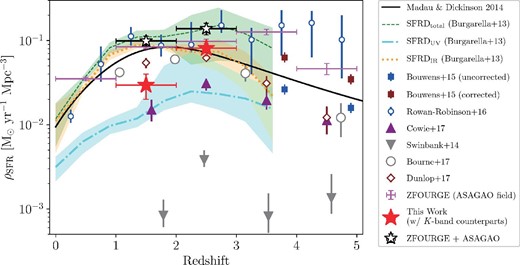
Contribution of ASAGAO sources to the cosmic SFRD as a function of redshift. Red, magenta, and black symbols are the contributions of ASAGAO sources with K-band counterparts, ALMA non-detected ZFOURGE sources within the ASAGAO field, and their sum, respectively. We adopt simple Poisson errors and SFR-errors attributed to redshift uncertainties. The black solid line indicate the recent results of the redshift evolution of the cosmic SFRD obtained by Madau and Dickinson (2014). The green dashed line, cyan dot–dashed line, and orange dotted line show the total (i.e., UV + IR) SFRD, UV SFRD, and IR SFRD obtained by Burgarella et al. (2013). Blue and brown squares are dust-uncorrected and -corrected SFRD obtained by Bouwens et al. (2015). Blue open circles are results of Rowan-Robinson et al. (2016). Purple triangles and gray open circles indicate the cosmic SFRD obtained by the SCUBA2 large survey by Cowie et al. (2017) and Bourne et al. (2017). The gray inverted triangles are the contribution of bright ALESS sources (Swinbank et al. 2014). Brown open diamonds indicate the contribution of the ALMA sources obtained by Dunlop et al. (2017). We note that these results are converted to the Chabrier IMF. (Color online)
As a comparison, we plot the recent parametric descriptions of the redshift evolution of the cosmic SFRD obtained by Madau and Dickinson (2014). Their results are based on the previous observations at UV-to-IR wavelengths. We also show the evolution of the cosmic SFRD at |$z$| = 0–3.5 derived by Burgarella et al. (2013). They use UV and IR luminosity functions estimated by the VIMOS-VLT Deep Survey (VVDS; Le Fèvre et al. 2005), the Herschel large programs PACS evolutionary probe (PEP; Lutz et al. 2011), and the Herschel Multi-tiered Extragalactic Survey (HerMES; Oliver et al. 2012) to estimate the cosmic SFRD. At |$z$| = 3.8 and 4.9, we plot results of Bouwens et al. (2015). They assume UV luminosity functions estimated by HST data and dust correction based on the IRX–βUV relation of Meurer et al. (1999). We also plot results of Rowan-Robinson et al. (2016), which are based on Herschel/SPIRE 500 μm sources. We also show the results of the SCUBA2 large survey by Cowie et al. (2017) and Bourne et al. (2017), the contribution of bright ALESS sources by Swinbank et al. (2014), and the results from ALMA continuum surveys estimated by Dunlop et al. (2017). Figure 12 suggests that the contribution of ASAGAO sources to the cosmic SFRD is ≳ 1 dex larger than that of bright ALESS sources (Swinbank et al. 2014) at |$z$| ∼ 1–3.
As shown in figure 12, the shape of the contribution of the cosmic SFRD from the ASAGAO sources is similar to that of the previous observations. Figure 12 shows that our results are ≳ 1-dex smaller than the cosmic IR SFRD obtained by Burgarella et al. (2013) at 1 < |$z$| < 2. At these redshifts, galaxies with log (LIR/L⊙) ≲ 9–10 (i.e., fainter populations than our ALMA detection limit) seems to be the main contributors to the cosmic IR SFRD. On the other hand, our results are consistent with the cosmic IR SFRD by Burgarella et al. (2013) (figure 12) at 2 < |$z$| < 3. This implies that in the redshift range of 2 < |$z$| < 3, the most part of the cosmic IR SFRD predicted by Burgarella et al. (2013) seems to be explained by ASAGAO sources. This can be a consequence of the evolution of the characteristic luminosities (|$L^*_\mathrm{IR}$|) of IR luminosity functions (i.e., at high redshift, |$L^*_\mathrm{IR}$| becomes higher; Hatsukade et al. 2018). Nevertheless, the deduced IR SFRD by ASAGAO sources may be suffered from small statistics and/or field-to-field variance. A survey with much wider survey volume would be necessary to mitigate such issues.
6 Conclusions
In this paper, we report results of multi-wavelength analysis of ALMA 1.2 mm detected ZFOURGE sources using ASAGAO data. We find that 24 ZFOURGE sources are detected by ALMA with S/N > 4.5. Their median redshift (|$z$|median = 2.38 ± 0.14) is consistent with redshifts of faint SMGs with Sobs ≲ 1.0 mJy, although this value is lower than that of “classical” SMGs (|$z$|median ∼ 3.0). This difference can be caused by the redshift evolution of the IR luminosity function, although we have to note that this can be caused by selection effect.
Our SED fitting from optical to millimeter wavelengths suggest that ASAGAO sources mainly lie on the high-mass end of the main sequence of star-forming galaxies, although some ASAGAO sources show starburst-like features. On the other hand, the IRX–M*, IRX–SFR, and IRX–βUV relations of ASAGAO sources may imply that ALMA detected sources and non-detected sources have different dust properties (e.g., dust compositions and/or dust distribution) even if they show similar properties on the M*–SFR plane.
We resolve the contribution of dusty star-forming sources to the cosmic SFRD down to log (LIR/L⊙) ∼ 11, because of the high sensitivity and angular resolution of ALMA. We find that the ASAGAO sources with K-band counterparts are main contributors to the cosmic IR SFRD at 2 < |$z$| < 3.
Acknowledgements
We thank the anonymous referee for her/his through reading of the manuscript and comments, which improved the paper significantly. This paper makes use of the following ALMA data: ADS/JAO.ALMA#2015.1.00098.S, 2015.1.00543.S, and 2012.1.00173.S. ALMA is a partnership of ESO (representing its member states), NSF (USA), and NINS (Japan) together with NRC (Canada), NSC and ASIAA (Taiwan), and KASI (Republic of Korea) in cooperation with the Republic of Chile. The Joint ALMA Observatory is operated by ESO, AUI/NRAO, and NAOJ. Data analysis was partly carried out on the common-use data analysis computer system at the Astronomy Data Center (ADC) of the National Astronomical Observatory of Japan (NAOJ). Y. Yamaguchi is thankful for the Japanese Society for the Promotion of Science (JSPS) fellowship. This study was supported by the JSPS Grant-in-Aid for Scientific Research (S) JP17H06130 and the NAOJ ALMA Scientific Research Number 2017-06B. H. Umehata acknowledges support from the JSPS KAKENHI Grant Number JP20H01953. Y. Ao acknowledges support by the National Natural Science Foundation of China (NSFC) grant 11933011.
Appendix 1 The correspondence of IDs in previous papers to ASAGAO IDs
Ueda et al. (2018) and Fujimoto et al. (2018) also report results of ASAGAO continuum sources. Aravena et al. (2016), Dunlop et al. (2017), Franco et al. (2018), and Cowie et al. (2018) also observed the similar region of ASAGAO. In this section, we present the correspondence of their IDs to our ASAGAO IDs (table 3). There are no ALESS sources within the ASAGAO field.
Correspondence to previous ALMA surveys in GOODS-S.*
| ASAGAO ID | ID in previous studies |
|---|---|
| (1) | (2) |
| 1 | UDF1, AGS6, SGS22, U3, F3 |
| 2 | AGS1, SGS5, U1, F1 |
| 3 | AGS3, SGS9, U2, F2 |
| 4 | UDF2, AGS18, SGS25, U6, F6 |
| 5 | UDF3, ASPECS/C1, AGS12, SGS48, U8, F8 |
| 6 | SGS20, U4, F4 |
| 7 | SGS29, U5, F6 |
| 8 | AGS13, SGS40, U12, F10 |
| 9 | F9 |
| 10 | UDF4, F132 |
| 11 | F7 |
| 12 | UDF5, F322 |
| 13 | UDF6, F26 |
| 14 | UDF7, U7 |
| 15 | UDF11, F73 |
| 16 | UDF8, ASPECS/C2, F90 |
| 17 | U11 |
| 19 | U10, F11 |
| 23 | UDF13 |
| 26 | SGS54, F103 |
| 29 | F148 |
| 31 | F113 |
| 33 | F30 |
| 44 | SGS63, F66 |
Appendix 2 ASAGAO ID21
We show the multi-wavelength “postage stamp” of ASAGAO ID21 in figure 13. ASAGAO ID 21 has “use flag =0” in Straatman et al. (2016). This is the reason why we remove this source from our analysis. However, we note that it has a spectroscopic redshift obtained by Wisnioski et al. (2015) (|$z$|spec = 2.187). For the case where we adopt this redshift and run the MAGPHYS, the best-fitted SED is shown in figure 14. Figure 14 shows that the stellar light is dominating the fit and the far-IR to millimeter spectrum is hugely underpredicted. This implies that the far-IR to millimeter bright region can lie at higher redshift than the optical/near-IR identified region. A chance alignment of (and perhaps associated gravitational amplification of) a dusty background galaxy with a physically unrelated galaxy in the foreground (e.g., Bourne et al. 2014; Oteo et al. 2017) could be responsible for the catastrophic SED fit.
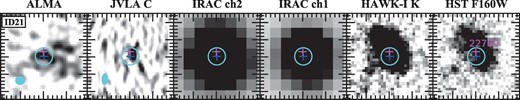
Multi-wavelength images of ASAGAO ID21. From left to right: ALMA 1.2 mm, JVLA 6 GHz, Spitzer IRAC/4.5 μm, IRAC/3.6 μm, VLT HAWK-I/Ks, and HST WFC3/F160W images. The field of view is 5″ × 5″. Blue and magenta crosses mark the ALMA positions and ZFOURGE positions, respectively. Cyan circles are 1″ apertures. The synthesized beams of ALMA and JVLA are expressed as filled ellipses.
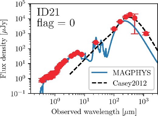
Estimated SEDs of ASAGAO ID21. Red symbols with errors are observed flux densities. Blue solid lines are best-fitting SEDs estimated by MAGPHYS. The black dashed lines are the mid-IR to far-IR SED model by Casey (2012).
Footnotes
Knudsen et al. (2008) suggest that the effective (source-plane) area within sufficient magnification to detect fainter (sub-)millimeter populations is only ∼0.1 arcmin2 for a typical rich cluster.
For example, S1.2 mm/S870 μm = 0.44, S1.2 mm/S1.3 mm = 1.26, and S1.2 mm/S1.1 mm = 0.79 at |$z$| = 2.83, 2.04, and 2.54 (median redshifts of ALESS, HUDF, and GOODS-ALMA sources).
This value is obtained by the SED fitting in Hsu et al. (2014).
The median redshift of ALMA non-detected ZFOURGE sources is |$z$|median = 1.45 ± 0.04.
For example, according to the ALMA Cycle 3 proposer’s guide, the absolute flux calibration uncertainty of Band 6 data is expected to be |$< 10\%$|.
We remove ID1 and ID7 because of large p-values, ID18 because of large discrepancy between its flux density at 1.2 mm and the best-fitting SED (figure 5), ID33 because of the number of photometry points less than 12 (figure 5). Note that ID18 may be affected by gravitational lensing by a chance coincidence of a foreground source. See also ID21 in appendix 2.
Although MAGPHYS provides IR luminosities in the range of 3–1000 μm in the rest-frame, the IR luminosities by MAGPHYS can be directly compared with other estimates referring to the commonly used wavelength range 8–1000 μm in the rest-frame. This is because the contribution of dust to the emission in the range of 3–8 μm is very small, as discussed in Clemens et al. (2013).
Herein we only use the star-forming galaxies selected by the UVJ-technique, as presented by Whitaker et al. (2011).
References
