


Abstract
The potential association between the blazar TXS 0506+056 and the neutrino event IceCube-170922A provides a unique opportunity to study the possible physical connection between high-energy photons and neutrinos. We explore the correlated electromagnetic and neutrino emissions of blazar TXS 0506+056 by a self-consistent leptonic–hadronic model, taking into account particle stochastic acceleration and all relevant radiative processes self-consistently. The electromagnetic and neutrino spectra of blazar TXS 0506+056 are reproduced by the proton synchrotron and hybrid leptonic–hadronic models based on the proton–photon interactions. It is found that the hybrid leptonic–hadronic model can be used to better explain the observed X-ray and |$\gamma$|-ray spectra of blazar TXS 0506+056 than the proton synchrotron model. Moreover, the predicted neutrino spectrum of the hybrid leptonic–hadronic model is closer to the observed one compared to the proton synchrotron model. We suggest that the hybrid leptonic–hadronic model is more favored if the neutrino event IceCube-170922A is associated with the blazar TXS 0506+056.
1 Introduction
Neutrino observation by IceCube has opened up a new window in the study of nonthermal processes in astrophysical objects. However, the sources responsible for the neutrino emission have not been identified so far. As neutrinos are not absorbed when interacting with the background photons or matter, they can be detected even though the source is far away. The observed distribution of their arrival direction suggests a predominantly extragalactic origin. Extragalactic sources, such as active galactic nuclei (Murase et al. 2014; Petropoulou 2015; Padovani 2016; Gao et al. 2017; Murase et al. 2018; Gao et al. 2019), |$\gamma$|-ray burst (Murase et al. 2006; Petropoulou 2014), and supernova (Murase et al. 2011; Petropoulou 2017), have been proposed as potential high-energy neutrino sources. Blazars are believed to be the most promising candidate sources with high-energy neutrino emission.
The IceCube observation recently reported the detection of a neutrino event (IceCube-170922A) coincident with the blazar TXS 0506+056 during its flaring state (IceCube Collaboration (2018a), 2018b). Following the neutrino alert, the blazar TXS 0506+056 was detected in a multi-wavelength campaign, ranging from the radio to |$\gamma$|-ray bands (IceCube Collaboration 2018b). The multi-wavelength observations characterize the polarization, variability, and energy spectrum of the blazar TXS 0506+056. This source was also first detected in very high-energy |$\gamma$|-ray bands with the MAGIC Cherenkov telescopes. A chance coincidence of a high-energy neutrino with a multi-wavelength flare is rejected at a 3.5 |$\sigma$| level. The potential association between the activity of TXS 0506+056 and the neutrino event suggests that this object could be the counterpart of a neutrino event.
Blazars are a subclass of radio-loud active galactic nuclei powered by supermassive black holes. Their radiation is thought to originate in a relativistic jet oriented at a small angle with respect to the line of sight. Blazars are often classified into BL Lac objects and flat spectrum radio quasars (FSRQs). BL Lacs have weak or absent emission lines, while FSRQs usually show strong broad emission lines. The spectrum energy distributions (SEDs) of blazars are characterized by nonthermal continuum spectra with a broad low-energy component from radio-UV to X-ray and a broad high-energy component from X-ray to |$\gamma$|-ray. It is generally accepted that the low-energy component of blazar SEDs is produced by synchrotron emission from relativistic electrons accelerated in the blazar jet. The high-energy component is often interpreted as the inverse Compton (IC) upscattering of ambient soft photons by the accelerated electrons (e.g., Böttcher 2007). The soft photons can be either synchrotron photons within the jet (the synchrotron self-Compton, SSC, process; Maraschi et al. 1992; Bloom & Marscher 1996), or the photons external to the jet (the external Compton, EC, process). These external photons may be the UV accretion disk photons (Dermer & Schlickeiser 1993), the accretion disk photons reprocessed by broad-line region clouds (Sikora et al. 1994), or infrared photons from the dust torus (Blaźejowski et al. 2000). The above scenario is called the leptonic model. Such models have achieved great successes in explaining the multi-wavelength emission and variability from blazars (Böttcher & Chiang 2002; Weidinger & Spanier 2010).
It is physically plausible that the protons are co-accelerated with the electrons to very high energy by the same mechanism in the jet of the blazar. In the so-called hadronic model, the synchrotron emission from the high-energy proton can dominate the high-energy component in the SED of blazars (Mannheim 1993; Mücke et al. 2003). Moreover, the high-energy protons can interact with the background photons to produce secondary electrons, and the synchrotron emission from the secondary electrons can have a significant contribution to the high-energy component (Petropoulou & Mastichiadis 2012; Mastichiadis et al. 2013; Cerruti et al. 2015; Weidinger & Spanier 2015; Diltz & Böttcher 2016; Zech et al. 2017). The high-energy component can also be produced by the |$\pi ^{0}$| decay from the proton–photon (|$p\gamma$|) interactions (Sahu et al. 2013; Cao & Wang 2014). For a recent review on blazar hadronic modeling, see Böttcher et al. (2013).
IceCube observation implied that the blazar TXS 0506+056 could be a high-energy neutrino source. Neutrinos are generally associated with the hadronic processes in the jet of the blazar. High-energy neutrinos can be produced by the decay of charged pions from the |$p\gamma$| interaction. Therefore, neutrinos can be considered as the unique signature of these hadronic interactions. A recent study revealed that the multi-TeV gamma-rays of blazars can be well explained by the photohadronic process, which provides strong evidence that the neutrino emission from blazars may originate in the photohadronic process (Sahu et al. 2019). In this paper we study the correlated electromagnetic and neutrino emissions of blazar TXS 0506+056 by a self-consistent leptonic–hadronic model, taking into account both electrons and protons, stochastic acceleration, and all relevant radiative processes self-consistently. We reproduce the electromagnetic and neutrino emissions of blazar TXS 0506+056 by the proton synchrotron and hybrid leptonic–hadronic models based on the |$p\gamma$| interaction. We demonstrate that the observed neutrino signature can allow us to distinguish these different emission models.
In section 2 we give a brief description of the model. In section 3 we apply the model to explain the electromagnetic and neutrino emissions of blazar TXS 0506+056. A discussion and the conclusion are presented in section 4. Throughout this paper we adopt the cosmological parameters of |$H_0 = 70$| km s|$^{-1}$| Mpc|$^{-1}$|, |$\Omega _M = 0.3$|, |$\Omega _{\Lambda } = 0.7$|.
2 Model
2.1 Model geometry
In this section we give a brief description of the model introduced by Weidinger and Spanier (2015). We improve their model by implementing the kinetic equation of the neutrinos and the Bethe–Heitler process. For a detail description of the model see Weidinger and Spanier (2010, 2015).
The model assumes a spherical geometry with two zones, where an acceleration zone with radius |$R_{\rm acc}$| is nested within a larger radiation zone with a radius |$R_{\rm rad}$|. Both zones are assumed to be homogeneous and to contain isotropic electron and proton distributions as well as a randomly oriented magnetic field. The considered blob travels down the jet axis towards the observer with a bulk Lorentz factor |$\Gamma$|, the upstream material is picked up into the acceleration zone where a highly turbulent zone is formed at the edge of the blob. Here, both injected particle species are subjected to stochastic acceleration processes up to relativistic energies, balanced by their radiation losses. However, the acceleration is assumed to be inefficient in the considerably larger radiation zone. The kinetic equations for each particle species i in each zone can be derived from the relativistic Vlasov equation (Schlickeiser 2002) by one-dimensional diffusion approximation using the relativistic approximation |$p_{i}=m_{i}c$|. Since blazar jets are almost aligned with the line of sight of the observer, we assume the Doppler factor |$\delta \simeq \Gamma$|. All calculations are conveniently made in the rest-frame of the blob.
2.2 Kinetic equation in the acceleration zone
2.3 Kinetic equation in the radiation zone
As every escaping particle from the acceleration zone enters the radiation region, the particle spectrum |$n_{i}(\gamma )$| from the acceleration zone serves as the injection function of the radiation zone. The particles are not accelerated in the radiation zone. Therefore, all relevant cool processes have to be taken into account, including synchrotron, inverse Compton and photo-hadronic losses. The kinetic equations for electrons, protons, photons, secondary positrons, and neutrinos are solved self-consistently and in a time-dependent fashion.
Note that no accelerated primary positrons are assumed in the model (|$n_{e^{+}}=0$|). The inverse Compton loss rate |$P_{{\rm IC}}$| is calculated using the full Klein–Nishina cross section given by Blumenthal and Gould (1970). The secondary pair production rate |$Q_{{\rm p}\gamma }$| from the |$p\gamma$| interaction is calculated using the |$\Phi _{\pm }$| parameters of the full SOPHIA Monte Carlo calculations carried out by Kelner and Aharonian (2008). The secondary pair production |$Q_{{\gamma \gamma }}$| from the |$\gamma \gamma$| interactions is calculated using the approximation of Aharonian, Atoyan, and Nagapetyan (1983). The photon pair production rate |$Q_{\rm BH}$| is calculated using the exact result of Kelner and Aharonian (2008).
2.4 Numeric method
To obtain the model SEDs, we numerically solve a set of coupled kinetic equations in the acceleration and radiation zones. In the acceleration zone, we use the method of Chang and Copper (1970) to solve equations (3). In the radiation zone, we use the method of Chiaberge and Ghisellini (1999) to solve equations (7), (9), and (10). Equations (11) and (12) are solved using the Crank–Nicotson method (Crank & Nicotson 1996). We carefully tested our numerical code with some analytical solutions and found very good agreement.
3 Results
The blazar TXS 0506+056 is a bright BL Lac object. The redshift of the source was recently measured to be |$z=0.337$| (Paiano et al. 2018). In 2017 September, IceCube reported a very high-energy muon neutrino event (IceCube-170922A), which was identified by the Extremely High Energy track event selection. The best-fit reconstructed direction is |$0.^{\!\!\!\circ }1$| from the sky position of the BL Lac object TXS 0506+056. The energy of the neutrino event is estimated to be 290 TeV with 90% confidence level lower limits of 183 TeV and upper limits of 4.3 PeV, by assuming a power-law neutrino spectrum with a spectral index of |$-2$|. The blazar TXS 0506+056 is a |$\gamma$|-ray source included in the third Fermi-LAT catalog of sources (Acero et al. 2015). Following the IceCuble alert, Fermi-LAT reported that the direction of IceCube-170922A is coincident with the location of TXS 0506+056 and coincident with the state of the |$\gamma$|-ray flare (Tanaka et al. 2017). Follow-up observations were performed by a multi-wavelength campaign with different telescopes, including a significant detection by MAGIC telescopes at |$>$|100 GeV, X-ray emissions by Swift/XRT and NuSTAR, optical emissions by the ASAS-SN survey, as well as emissions in the radio band by VLA (see IceCube Collaboration 2018b). The high-energy neutrinos originating in the hadronic interactions provided a natural link between the high-energy |$\gamma$|-rays and neutrinos. The combined multi-wavelength and neutrino observations provide a unique opportunity to study the hadronic processes in blazar jets.
We use the model described in section 2 to model the electromagnetic and neutrino spectra of blazar TXS 0506+056. The observed data is taken from IceCube Collaboration (2018b). We interpret the electromagnetic and neutrino spectra of blazar TXS 0506+056 by proton synchrotron and hybrid leptonic–hadronic models. In figure 1, we show the predicted electromagnetic and neutrino spectra for the proton synchrotron model. The modeling parameters are listed in table 1. The derived SEDs are corrected for extragalactic background light (EBL) absorption using the models of Franceschini, Rodighiero, and Vaccari (2008) and Finke, Razzaque, and Dermer (2010). The different EBL models predict a similar |$\gamma$|-ray spectrum, and the differences between them are negligible. It can be seen that the optical and Swift X-ray spectra are produced by the synchrotron radiation of the primary electron, the NuSTAR X-ray spectrum comes from the low-energy tail of the proton synchrotron radiation, and the high-energy |$\gamma$|-ray spectrum is dominated by proton synchrotron radiation. In fact, the contribution of the secondary emission from the pair cascades to the |$\gamma$|-ray spectrum is negligible due to strong EBL absorption above |$10^{26}$| Hz. We note that the SSC emission from the primary electrons and the synchrotron emission of the secondary pairs from the Bethe–Heitler process have a negligible contribution to the observed SEDs due to the high magnetic field of |$\mathcal {O}$|(10 G) (see table 1). The peak energy of the predicted neutrino spectrum is |${\sim } 10^{32}$| Hz, which is far above the observed neutrino energy. In figure 2 we show the proton, electron, and positron spectra from the derived SEDs in figure 1. In the acceleration zone, the stochastic acceleration process produces a power-law proton injected spectrum with index |$q_{\rm p}\simeq 1+t_{\rm acc,p}/(2\, t_{\rm esc,p})=1.525$|. In the radiation zone, the proton synchrotron loss dominates over the photo–meson loss due to the high magnetic field. Therefore, the synchrotron cooling results in a power-law proton spectrum with index |$n_{\rm p}\simeq q_{\rm p}+1=2.525$| above the break energy |$\gamma _{\rm b,p}\simeq 1/(t_{\rm esc,rad,p}\, \beta _{\rm s,p})=5\times 10^6$|. The maximum proton energy can be determined by |$\gamma _{\rm max,p}\simeq 1/(t_{\rm esc,p}\, \beta _{\rm s,p})=2\times 10^9$|. The peak energy of proton synchrotron radiation is |$\nu ^{\rm obs}_{\rm s,p}\simeq 4.2\times 10^6 \delta \, B \, (m_{e}/m_{\rm p}) \, \gamma ^2_{\rm max,p}=5\times 10^{24}$| Hz, which is comparable with the value from the model-derived SED (see figure 1). The electron density with |$\gamma >10^{4}$| is the contribution of the secondary electrons from the pair cascade processes, because the primary electrons cannot be accelerated to such high energies. We note that the X-ray and |$\gamma$|-ray data cannot be reproduced well by the proton synchrotron model.
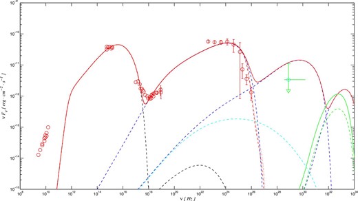
Predicted multi-wavelength flux and neutrino flux of TXS 0506+056 for the proton synchrotron model. The red circles are the observed multi-wavelength data and the green circle is the detected neutrino flux from the IceCube observation. The black dashed curves represent the synchrotron emission and the SSC emission, respectively (from left to right). The blue dashed curves represent the proton synchrotron emission, the synchrotron emission from the secondary pairs, and the |$\gamma$|-ray emission from |$\pi ^{0}$| decay, respectively (from left to right). The cyan dashed curves represent the synchrotron emission of the secondary pairs from the Bethe–Heitler process. The green dashed curve represents the muon neutrino spectrum from the charged pion decay. The all-flavor neutrino spectrum is also shown as the green solid curve. The red solid curve is the total spectrum from all emission components, while the red dashed curve is the EBL-corrected spectrum using the EBL model of Finke, Razzaque, and Dermer (2010). For comparison, The EBL-corrected spectrum using the EBL model of Franceschini, Rodighiero, and Vaccari (2008) is also shown as the red dotted curve. The observed data are taken from IceCube Collaboration (2018b). (Color online)
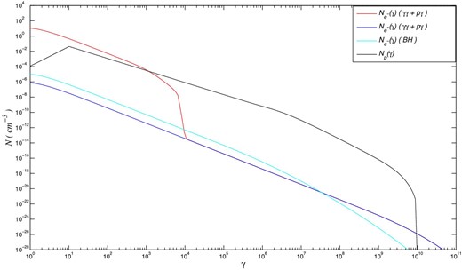
Proton, electron, and positron spectra from the derived SEDs in figure 1. (Color online)
Model parameters of the proton synchrotron process.
| Parameters | |
|---|---|
| B (G) | 10 |
| |$\delta _{\rm D}$| | 48 |
| |$\gamma _{\, 0,e}$| | |$6.0\times 10^{3}$| |
| |$Q_{\, 0,e}$| (cm|$^{-3}$| s|$^{-1}$|) | |$1.6\times 10^{-1}$| |
| |$\gamma _{\, \rm 0,p}$| | 10 |
| |$Q_{\, \rm 0,p}$| (cm|$^{-3}$| s|$^{-1}$|) | |$4.0\times 10^{-3}$| |
| |$R_{\, \rm acc}$| (cm) | |$3.0\times 10^{13}$| |
| |$R_{\, \rm rad}$| (cm) | |$1.6\times 10^{16}$| |
| |$t_{\, \rm acc}/t_{\rm esc}$| | 1.05 |
In figure 3 we show the predicted electromagnetic and neutrino spectra for the hybrid leptonic–hadronic model. In figure 4 we show the proton, electron, and positron spectra from the derived SEDs in figure 3. The modeling parameters are listed in table 2. It can be seen that the optical and Swift X-ray spectra come from the synchrotron radiation of the primary electron. The NuSTAR X-ray spectrum is produced by the combination of the SSC radiation and the synchrotron radiation of the secondary pairs from the Bethe–Heitler processes. The high-energy |$\gamma$|-ray spectrum comes from the combination of the SSC radiation and the synchrotron radiation from the secondary pairs. We note that the synchrotron radiation from the secondary pairs mainly contributes to the high-energy tails of the |$\gamma$|-ray spectrum. In fact, the proton synchrotron radiation makes a negligible contribution to the observed SEDs due to the low magnetic field of |$\mathcal {O}$|(1 G) (see table 2). The neutrino peak energy can be estimated by the maximum proton energy from the relation |$E_{\nu }=0.05 \, E_{\rm max,p}$|. Therefore, the corresponding neutrino peak frequency is |$\nu ^{\rm obs}_{\nu }\simeq 3\times 10^{29}(\gamma _{\rm max,p}/10^6)(\delta /28)$| Hz, which is closer to the observed neutrino energy compared to the proton synchrotron emission. Recently, a study by the MAGIC collaboration showed that the blazar TXS 0506+056 has a Doppler factor of about 40 (Ansoldi et al. 2018). We also show the predicted electromagnetic and neutrino spectra for a high Doppler factor (|$\delta =40$|) as the solid curves in figure 5. The modeling parameters are listed in table 3. For comparison, the predicted electromagnetic and neutrino spectra for a low Doppler factor (|$\delta =28$|) are also shown as the dashed curves. It is found that the model of the high Doppler factor predicts a slightly higher neutrino flux than the low Doppler factor. Our results imply that the hybrid leptonic–hadronic model can better match the X-ray and |$\gamma$|-ray spectra than the proton synchrotron model (see figures 1 and 5).
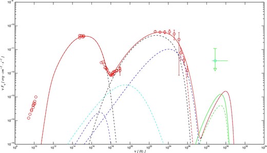
As figure 1, but for the hybrid leptonic–hadronic model. (Color online)

Proton, electron, and positron spectra from the derived SEDs in figure 3. (Color online)
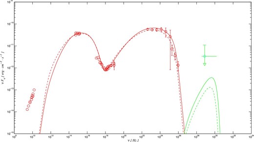
As figure 3, but for a different Doppler factor. The solid curves represent the predicted electromagnetic and neutrino spectrum for a high Doppler factor (|$\delta =40$|). For comparison, the predicted electromagnetic and neutrino spectra for a low Doppler factor (|$\delta =28$|) are also shown as the dashed curves. (Color online)
Model parameters of the leptonic–hadronic process.
| Parameters | |
|---|---|
| B (G) | 0.95 |
| |$\delta _{\rm D}$| | 28 |
| |$\gamma _{\, 0,e}$| | |$1.5\times 10^{3}$| |
| |$Q_{0,e}$| (cm|$^{-3}$| s|$^{-1}$|) | |$1.8\times 10^{-1}$| |
| |$\gamma _{\, \rm 0,p}$| | |$10^2$| |
| |$Q_{\, \rm 0,p}$| (cm|$^{-3}$| s|$^{-1}$|) | |$1.4\times 10^{-3}$| |
| |$R_{\, \rm acc}$| (cm) | |$1.0\times 10^{14}$| |
| |$R_{\, \rm rad}$| (cm) | |$5.5\times 10^{15}$| |
| |$t_{\, \rm acc}/t_{\rm esc}$| | 1.2 |
Model parameters of the leptonic–hadronic process for a high Doppler factor.
| Parameters | |
|---|---|
| B (G) | 1 |
| |$\delta _{\rm D}$| | 40 |
| |$\gamma _{\, 0,e}$| | |$1.5\times 10^{3}$| |
| |$Q_{\, 0,e}$| (cm|$^{-3}$| s|$^{-1}$|) | |$5.6\times 10^{-2}$| |
| |$\gamma _{\, \rm 0,p}$| | |$10^2$| |
| |$Q_{\, \rm 0,p}$| (cm|$^{-3}$| s|$^{-1}$|) | |$2.3\times 10^{-3}$| |
| |$R_{\, \rm acc}$| (cm) | |$1.0\times 10^{14}$| |
| |$R_{\, \rm rad}$| (cm) | |$2.5\times 10^{15}$| |
| |$t_{\, \rm acc}/t_{\rm esc}$| | 1.3 |
4 Discussion and conclusions
Proton–proton (|$pp$|) interactions have been invoked to explain the observed neutrino spectrum of blazar TXS 0506+056 (Wang et al. 2018; He et al. 2018; Sahakyan 2018; Liu et al. 2019). The |$pp$| interaction usually requires a high plasma density, which is not expected in the environment of BL Lac objects due to the small accretion rate (Aharonian 2000). The observed neutrino spectrum can be explained by |$p\gamma$| interactions with an external radiation field (Keivani et al. 2018). It is thought that BL Lac objects lack a strong external radiation field due to the clean environment around the jet. A steady leptonic–hadronic model was used to study the electromagnetic and neutrino emissions of blazar TXS 0506+056 (Cerruti et al. 2018; Zhang et al. 2018). However, these models do not include the particle acceleration and the relevant radiative processes self-consistently.
In this paper we studied the correlated electromagnetic and neutrino emission of blazar TXS 0506+056 with a self-consistent leptonic–hadronic model, taking into account both electron and proton acceleration and all relevant radiative processes self-consistently. We have reproduced the electromagnetic and neutrino spectra of blazar TXS 0506+056 with the proton synchrotron and hybrid leptonic–hadronic models based on the |$p\gamma$| interaction. We find that the hybrid leptonic–hadronic model can better reproduce the observed multi-wavelength SEDs of blazar TXS 0506+056. Moreover, the predicted neutrino spectrum of the hybrid leptonic–hadronic model is closer to the observed one compared to the proton synchrotron model. Therefore, we suggest that the hybrid leptonic–hadronic model is more preferred if the neutrino IceCube-170922A originates from blazar TXS 0506+056. It is not possible to put a strong constraint on neutrino production models with a single observed neutrino event. Further multi-messenger observations will be needed to understand the possible physical connection between the neutrino and |$\gamma$|-ray emissions.
Acknowledgments
We thank the anonymous referee for valuable comments and suggestions. We acknowledge the financial support from the National Natural Science Foundation of China 11573060 and 11663008, the National Science Foundation of China 11673060, and the Natural Science Foundation of Yunnan Province under grant 2016FB003.
References
