Doppler tomographic measurement of the nodal precession of WASP-33b

Parameters of WASP-33 from the previous literature.

Parameter	Value	Reference
Planetary parameter
λ₂₀₀₈ (°)	\|$-110.06^{+0.40}_{-0.47}$\|	Johnson et al. (2015)
λ₂₀₁₄ (°)	\|$-112.93^{+0.23}_{-0.21}$\|	Johnson et al. (2015)
b ₂₀₀₈	\|$0.218^{+0.011}_{-0.029}$\|	Johnson et al. (2015)
b ₂₀₁₄	\|$0.0840^{+0.0020}_{-0.0019}$\|	Johnson et al. (2015)
R _p/R_s	0.1143 ± 0.0002	Collier Cameron et al. (2010)
a/R_s	3.69 ± 0.01	Collier Cameron et al. (2010)
P (d)	1.2198675 ± 0.0000011	von Essen et al. (2014)
T _c (BJD_TDB)	2456878.65739 ± 0.00015	von Essen et al. (2019)
v _FWHM* (km s⁻¹)	16.2 ± 0.5 (TLS)^†	Collier Cameron et al. (2010)
	19.2 ± 0.6 (McD)^†	Collier Cameron et al. (2010)
	18.1 ± 0.3 (NOT)^†	Collier Cameron et al. (2010)
Stellar parameter
V sin i_⋆ (km s⁻¹)	\|$86.63^{+0.37}_{-0.32}$\|	Johnson et al. (2015)
log g (cgs)	4.3 ± 0.2	Collier Cameron et al. (2010)
T _eff (K)	7430 ± 100	Collier Cameron et al. (2010)
Fe\|$/$\|H	0.10 ± 0.2	Collier Cameron et al. (2010)

Parameter	Value	Reference
Planetary parameter
λ₂₀₀₈ (°)	\|$-110.06^{+0.40}_{-0.47}$\|	Johnson et al. (2015)
λ₂₀₁₄ (°)	\|$-112.93^{+0.23}_{-0.21}$\|	Johnson et al. (2015)
b ₂₀₀₈	\|$0.218^{+0.011}_{-0.029}$\|	Johnson et al. (2015)
b ₂₀₁₄	\|$0.0840^{+0.0020}_{-0.0019}$\|	Johnson et al. (2015)
R _p/R_s	0.1143 ± 0.0002	Collier Cameron et al. (2010)
a/R_s	3.69 ± 0.01	Collier Cameron et al. (2010)
P (d)	1.2198675 ± 0.0000011	von Essen et al. (2014)
T _c (BJD_TDB)	2456878.65739 ± 0.00015	von Essen et al. (2019)
v _FWHM* (km s⁻¹)	16.2 ± 0.5 (TLS)^†	Collier Cameron et al. (2010)
	19.2 ± 0.6 (McD)^†	Collier Cameron et al. (2010)
	18.1 ± 0.3 (NOT)^†	Collier Cameron et al. (2010)
Stellar parameter
V sin i_⋆ (km s⁻¹)	\|$86.63^{+0.37}_{-0.32}$\|	Johnson et al. (2015)
log g (cgs)	4.3 ± 0.2	Collier Cameron et al. (2010)
T _eff (K)	7430 ± 100	Collier Cameron et al. (2010)
Fe\|$/$\|H	0.10 ± 0.2	Collier Cameron et al. (2010)

*v_FWHM is the FWHM of the instinct profile assumed as a Gaussian line.

^†TLS: Thüringer Landessternwarte Tautenburg; McD: McDonald Observatory; NOT: Nordic Optical Telescope.

Table 1.

Parameters of WASP-33 from the previous literature.

Parameter	Value	Reference
Planetary parameter
λ₂₀₀₈ (°)	\|$-110.06^{+0.40}_{-0.47}$\|	Johnson et al. (2015)
λ₂₀₁₄ (°)	\|$-112.93^{+0.23}_{-0.21}$\|	Johnson et al. (2015)
b ₂₀₀₈	\|$0.218^{+0.011}_{-0.029}$\|	Johnson et al. (2015)
b ₂₀₁₄	\|$0.0840^{+0.0020}_{-0.0019}$\|	Johnson et al. (2015)
R _p/R_s	0.1143 ± 0.0002	Collier Cameron et al. (2010)
a/R_s	3.69 ± 0.01	Collier Cameron et al. (2010)
P (d)	1.2198675 ± 0.0000011	von Essen et al. (2014)
T _c (BJD_TDB)	2456878.65739 ± 0.00015	von Essen et al. (2019)
v _FWHM* (km s⁻¹)	16.2 ± 0.5 (TLS)^†	Collier Cameron et al. (2010)
	19.2 ± 0.6 (McD)^†	Collier Cameron et al. (2010)
	18.1 ± 0.3 (NOT)^†	Collier Cameron et al. (2010)
Stellar parameter
V sin i_⋆ (km s⁻¹)	\|$86.63^{+0.37}_{-0.32}$\|	Johnson et al. (2015)
log g (cgs)	4.3 ± 0.2	Collier Cameron et al. (2010)
T _eff (K)	7430 ± 100	Collier Cameron et al. (2010)
Fe\|$/$\|H	0.10 ± 0.2	Collier Cameron et al. (2010)

Parameter	Value	Reference
Planetary parameter
λ₂₀₀₈ (°)	\|$-110.06^{+0.40}_{-0.47}$\|	Johnson et al. (2015)
λ₂₀₁₄ (°)	\|$-112.93^{+0.23}_{-0.21}$\|	Johnson et al. (2015)
b ₂₀₀₈	\|$0.218^{+0.011}_{-0.029}$\|	Johnson et al. (2015)
b ₂₀₁₄	\|$0.0840^{+0.0020}_{-0.0019}$\|	Johnson et al. (2015)
R _p/R_s	0.1143 ± 0.0002	Collier Cameron et al. (2010)
a/R_s	3.69 ± 0.01	Collier Cameron et al. (2010)
P (d)	1.2198675 ± 0.0000011	von Essen et al. (2014)
T _c (BJD_TDB)	2456878.65739 ± 0.00015	von Essen et al. (2019)
v _FWHM* (km s⁻¹)	16.2 ± 0.5 (TLS)^†	Collier Cameron et al. (2010)
	19.2 ± 0.6 (McD)^†	Collier Cameron et al. (2010)
	18.1 ± 0.3 (NOT)^†	Collier Cameron et al. (2010)
Stellar parameter
V sin i_⋆ (km s⁻¹)	\|$86.63^{+0.37}_{-0.32}$\|	Johnson et al. (2015)
log g (cgs)	4.3 ± 0.2	Collier Cameron et al. (2010)
T _eff (K)	7430 ± 100	Collier Cameron et al. (2010)
Fe\|$/$\|H	0.10 ± 0.2	Collier Cameron et al. (2010)

*v_FWHM is the FWHM of the instinct profile assumed as a Gaussian line.

^†TLS: Thüringer Landessternwarte Tautenburg; McD: McDonald Observatory; NOT: Nordic Optical Telescope.

In this paper we report on additional Doppler tomographic measurement of WASP-33b. In section 2 we summarize our data sets and the methods used to calculate the orbital obliquity and impact parameter from the data. Next, we show the results of our analysis in section 3. We examine how WASP-33b’s nodal precession behaves from our results in section 4. Finally, we present the conclusion of this paper in section 5.

2 Methods

2.1 Spectroscopic data sets

We used three archival spectroscopic data sets of WASP-33 around planetary transits. One of them was taken by the 8.2 m Subaru telescope with High Dispersion Spectrograph (HDS; Noguchi et al. 2002) on 2011 October 19 UT. The others are the data sets observed by the Harlan J. Smith Telescope (HJST) with the Robert G. Tull Coudé Spectrograph (TS23; Tull et al. 1995) at McDonald Observatory on 2008 November 12 UT (Collier Cameron et al. 2010) and 2014 October 4 UT (J+15).

The HDS data set includes 35 spectra obtained with a resolution of R = 110000; 16 spectra taken in transit. The exposure times are 600 s for 33 spectra and 480 s for 2 spectra. In this study we adopted a range of wavelengths from 4930 Å to 6220 Å, except for Na D lines and regions of wavelengths around bad pixels. From these spectra we took continua, corrected them to eliminate the Earth’s atmospheric dispersion by dividing spectra of a rapidly rotating star HR8634 (V sin I_⋆ ∼ 140 km s⁻¹; Abt et al. 2002), and shifted these spectra to the barycentric frame. For these processes we used PyRAF and the calculating tools from Wright and Eastman (2014) and Eastman, Siverd, and Gaudi (2010). Then we found that the signal-to-noise ratio (S/N) per pixel of each spectrum was ∼160 at 5500 Å. To pick up each line profile from each spectrum, we adopted least squares deconvolution (LSD; Donati et al. 1997). In this method we regard an observed spectrum as a convolution of a line profile and a series of delta functions. We referred to depths of about 1000 atomic absorption lines from the Vienna Atomic Line Database (VALD; Kupka et al. 2000) and considered these lines as delta functions. Then we derived all of the line profiles and their error bars by deconvolution using the matrix calculations in Kochukhov, Makaganiuk, and Piskunov (2010). Finally, we shifted these profiles by the velocity of this system, γ = −3.69 km s⁻¹ (Collier Cameron et al. 2010).

On the other hand, two data sets of TS23 have R = 60000 resolution. One data set for the 2008 epoch has 13 spectra and S/N per pixel of ∼140. The other set for the 2014 epoch has 21 spectra and S/N per pixel of ∼280. Both of these include 10 in-transit spectra. All of their exposure times are 900 s. We note that the two data sets have already been extracted and published in J+15, and we used the extracted line profile series.

2.2 Extracting planetary shadow

We computed a median line profile for each data set. We subtracted the median line profile from each line profile of each exposure to compute the time series of line profile residuals. In the time series of residuals there is not only a planetary shadow caused by WASP-33b’s transit, but also a striped pattern (see figure 1). The extra pattern occurs from non-radial pulsations on the surface of WASP-33 (Collier Cameron et al. 2010).

Fig. 1.

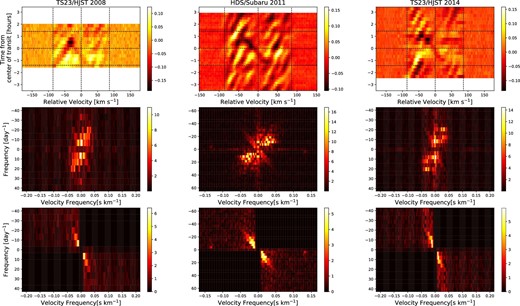
Doppler tomographic data sets and Fourier filters. The first, second, and third columns show the data sets of TS23 in 2008, HDS in 2011, and TS23 in 2014, respectively. Top row: Observed residuals of line profile series. The virtual dotted lines show v = 0, ±v sin i_⋆. The bottom, middle, and upper horizontal dotted lines show the beginning, middle, and end of WASP-33b’s transit, respectively. Second row: Fourier spaces after Fourier transform of the residuals of the line profile series. These color scales are shown in square roots. The faint narrow structure from the right bottom to the left upper is a component of WASP-33b’s planetary transit. On the other hand, the bright wide structure from the left bottom to the right upper is a component of pulsations. Third row: Filtered Fourier space so that only the transit component remains. (Color online)

To extract only the planetary shadow, we applied a Fourier filtering technique (J+15). First, we did a two-dimensional Fourier transform. Second, we made a filter which we set to unity in the two diagonal quadrants including power from the planetary shadow, and zero in the other quadrants including power from the pulsation, with a Hann function between these quadrants. Then, we multiplied the Fourier space by the filter and performed an inverse Fourier transform on the filtered Fourier space. These procedures are shown from top to bottom in figure 1.

2.3 Deriving parameters

To obtain best-fit values and uncertainties of the transit parameters we adopted a Markov chain Monte Carlo (MCMC) technique using the EMCEE program (Foreman-Mackey et al. 2013).

We modeled a planetary shadow by convolution between the equations in the appendix and a Gaussian line profile due to intrinsic broadening, thermal broadening, and microturbulence. We then applied the same filter to the planetary shadow model following the procedures described in subsection 2.2.

We fitted the observed residuals of the three data sets to the models with 15 parameters using MCMC: λ, b, and T_c of each epoch, V sin i_⋆, R_p/R_⋆, a/R_⋆, two quadratic limb-darkening coefficients, and the FWHM of the Gaussian line profile. Note that the limb-darkening coefficients are derived by the triangular sampling method of Kipping (2013), q₁ and q₂. Here we estimated that q₁ and q₂ for HDS and TS23 are equivalent. They can be calculated from the stellar parameters, i.e., the effective temperature T_eff, surface gravity log g, and metallicity. We set priors of λ and b for all epochs and the FWHM as uniform functions, otherwise as Gaussian priors. For the values and widths of the Gaussian priors we set the priors of R_p/R_⋆ and a/R_⋆ based on the values and uncertainties from Kovács et al. (2013), for the T_c of each epoch from P in von Essen et al. (2014) and T₀ in von Essen et al. (2019), for q₁ and q₂ calculated by PyLDTk (Husser et al. 2013; Parviainen & Aigrain 2015), and for V sin i_⋆ from J+15.

For the fitting, we minimized

$$\begin{eqnarray} \chi ^{2} = \sum _{i} \frac{(O_{i}-C_{i})^{2}}{\sigma ^{2}_{i}} + \sum _{j} \frac{(p_{j}-\mu _{j})^{2}}{s^{2}_{j}}, \end{eqnarray}$$

(1)

where O_i is the data, C_i is the model, σ_i is the error for the ith data point, p is the value of the parameter, μ is the value from the literature, and s is the uncertainty from the literature. The indices j and k denote the parameters for the Gaussian priors and the uniform priors, respectively. To converge the values of these parameters we ran 4000 steps, removed the first 2000 steps as burn-in, and iterated this set 100 times. The posterior distributions are plotted in figure 2.

Fig. 2.

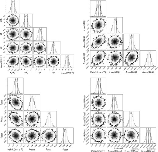
Corner plots for the free parameters after using MCMC as in subsection 2.3. The black circles indicate 68%, 95%, and 99.7% confidence from the inside. In each posterior distribution of each parameter, vertical dotted lines show its best-fit value (middle) and 1 σ confidence (both ends). We created these plots with corner.py (Foreman-Mackey 2016).

3 Results

We show the line profile residuals and the best-fit filtered models in figure 3. The best values of λ and b are listed in table 2. Our results for λ and b in 2014 are in excellent agreement with the values of J+15, whereas those from 2008 are marginally consistent with J+15 within 2 σ.

Fig. 3.

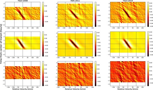
Fitting for filtered residual data by MCMC. These are the same type of color scale as the first row in figure 1. First row: Residual data containing only a planetary shadow. Second row: Filtered models of planetary shadow using best-fit values. Third row: Difference between the first row and the second row. (Color online)

Table 2.

Observed parameters.

Parameter	2008	2011	2014
λ (°)	\|$-111.28^{+0.47}_{-0.48}$\|	\|$-114.01^{+0.22}_{-0.20}$\|	−112.91 ± 0.24
b	\|$0.2397^{+0.0040}_{-0.0039}$\|	0.1571 ± 0.0020	\|$0.0856^{+0.0021}_{-0.0020}$\|
i _p (°)	\|$86.275^{+0.070}_{-0.072}$\|	87.560 ± 0.037	\|$88.671^{+0.034}_{-0.036}$\|
Ω (°)	\|$86.003^{+0.087}_{-0.091}$\|	87.329 ± 0.045	\|$88.557^{+0.039}_{-0.045}$\|
I (°)	\|$111.23^{+0.48}_{-0.47}$\|	\|$113.99^{+0.20}_{-0.22}$\|	112.90 ± 0.24

Parameter	2008	2011	2014
λ (°)	\|$-111.28^{+0.47}_{-0.48}$\|	\|$-114.01^{+0.22}_{-0.20}$\|	−112.91 ± 0.24
b	\|$0.2397^{+0.0040}_{-0.0039}$\|	0.1571 ± 0.0020	\|$0.0856^{+0.0021}_{-0.0020}$\|
i _p (°)	\|$86.275^{+0.070}_{-0.072}$\|	87.560 ± 0.037	\|$88.671^{+0.034}_{-0.036}$\|
Ω (°)	\|$86.003^{+0.087}_{-0.091}$\|	87.329 ± 0.045	\|$88.557^{+0.039}_{-0.045}$\|
I (°)	\|$111.23^{+0.48}_{-0.47}$\|	\|$113.99^{+0.20}_{-0.22}$\|	112.90 ± 0.24

Table 2.

Observed parameters.

Parameter	2008	2011	2014
λ (°)	\|$-111.28^{+0.47}_{-0.48}$\|	\|$-114.01^{+0.22}_{-0.20}$\|	−112.91 ± 0.24
b	\|$0.2397^{+0.0040}_{-0.0039}$\|	0.1571 ± 0.0020	\|$0.0856^{+0.0021}_{-0.0020}$\|
i _p (°)	\|$86.275^{+0.070}_{-0.072}$\|	87.560 ± 0.037	\|$88.671^{+0.034}_{-0.036}$\|
Ω (°)	\|$86.003^{+0.087}_{-0.091}$\|	87.329 ± 0.045	\|$88.557^{+0.039}_{-0.045}$\|
I (°)	\|$111.23^{+0.48}_{-0.47}$\|	\|$113.99^{+0.20}_{-0.22}$\|	112.90 ± 0.24

Parameter	2008	2011	2014
λ (°)	\|$-111.28^{+0.47}_{-0.48}$\|	\|$-114.01^{+0.22}_{-0.20}$\|	−112.91 ± 0.24
b	\|$0.2397^{+0.0040}_{-0.0039}$\|	0.1571 ± 0.0020	\|$0.0856^{+0.0021}_{-0.0020}$\|
i _p (°)	\|$86.275^{+0.070}_{-0.072}$\|	87.560 ± 0.037	\|$88.671^{+0.034}_{-0.036}$\|
Ω (°)	\|$86.003^{+0.087}_{-0.091}$\|	87.329 ± 0.045	\|$88.557^{+0.039}_{-0.045}$\|
I (°)	\|$111.23^{+0.48}_{-0.47}$\|	\|$113.99^{+0.20}_{-0.22}$\|	112.90 ± 0.24

We calculated other parameters for angles: Ω, the ascending node, and I, the inclination of the orbital plane with respect to the x–y plane (see figure 4). These angles can be calculated with the following equations:

$$\begin{eqnarray} \tan \Omega &=& -\sin \lambda \tan i_{\rm p}, \end{eqnarray}$$

(2)

$$\begin{eqnarray} \cos I &=& \cos \lambda \sin i_{\rm p}, \end{eqnarray}$$

(3)

where i_p is the angle between the line of sight and the momentum of the planetary orbit. We assumed that a/R_⋆ is constant at any time. The values of these calculated parameters are shown in table 2.

Fig. 4.

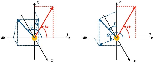
Outlines of the planetary system. We set the y axis as the line of sight and the x–z plane as the plane of the sky. The red and blue vectors show the stellar spin axis and the planetary orbital momentum respectively. (Color online)

4 Discussion

The angular momentum of WASP-33b’s planetary orbit L_p (= |$2 \pi M_{\rm p} a_{\rm p}^{2}/P$|⁠) is much smaller than the stellar rotational angular momentum of its host star L_⋆; L_p/L_⋆ is ∼0.05 using the values of L_⋆ from Iorio (2011), M_p from Lehmann et al. (2015), and a_p and P from Collier Cameron et al. (2010). In this case, we can regard the stellar rotational axis as a stable vector. According to equations (8) and (9) in Iorio (2016), the long-term change in Ω and I can be expressed as

$$\begin{eqnarray} \dot{\Omega } &=& -\frac{3 \pi J_{2} R_{\star }^{2}}{2 a^{2}P} [2 \sin i_{\star }\cos i_{\star }\cos 2I\csc I \cos \Omega\\ && - \cos I (1-3\sin ^{2} i_{\star }+\cos ^{2}i_{\star }\cos 2\Omega )], \end{eqnarray}$$

(4)

$$\begin{eqnarray} && \dot{I} = -\frac{3 \pi J_{2} R_{\star }^{2}}{a^{2}P}\cos i_{\star } \sin \Omega (\sin i_{\star }\cos I-\cos i_{\star }\sin I\cos \Omega ),\\ \end{eqnarray}$$

(5)

assuming that its orbit is circular and the stellar spin axis stays on the y–z plane in figure 4. These equations need to be solved numerically. Thus, we adopt the Euler method to fit equations (4) and (5) to our results with initial parameters of Ω and I in 2008 and Δt = 1 d. In this fitting we use the χ² fitting method, setting Ω and I at the 2008 epoch, and i_⋆ and J₂ as free parameters. We rescale the calculated errors of Ω and I so that |$\chi ^{2}_{\mathrm{min}}$| equals the number of degrees of freedom. Then we estimate the errors in i_⋆ and J₂ by |$\Delta \chi ^{2} (\equiv \chi ^{2}-\chi ^{2}_{\mathrm{min}}) = 1$|⁠.

Fitted time variations of Ω and I over long and short terms are shown in figure 5. We derive |$i_{\star }=96^{+10}_{-14}$| deg and J₂ = (9.14 ± 0.51) × 10⁻⁵, which means WASP-33 is viewed more equator-on and is more spherical than the results in Iorio (2016). We also estimate that the nodal precession period P_op is ∼840 yr, which is shorter than that estimated in J+15. Though three data points of Ω fit the model very well, deriving the rate of nodal precession in the short term dΩ/dt = 0.4269 ± 0.0051 deg yr⁻¹, those of I do not. This may imply that WASP-33b’s precession has a short-term variation, or the measured errors of I are underestimated.

Fig. 5.

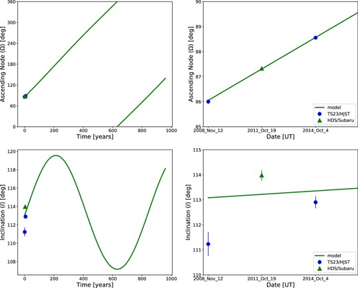
Changes of Ω (upper row) and I (lower row). The left and right columns show the change in the long and short term respectively. The x-axis of the left column is the time in years from the epoch of 2018. The blue circles show values from the data sets of HJST/TS23, whereas the green triangles are values from Subaru/HDS and the green solid lines are the model based on Iorio (2016). (Color online)

We also plot the changes of orbital inclination i_p and the impact parameter b in figure 6 based on the following equations:

$$\begin{eqnarray} \cos i_{\rm p} = \sin I \cos \Omega , \end{eqnarray}$$

(6)

$$\begin{eqnarray} b = (a/R_{\star }) \cos i_{\rm p} . \end{eqnarray}$$

(7)

We find that the amplitude of WASP-33b’s i_p is ∼67°. We also find that WASP-33b transits in front of the host star for only ∼20% of the whole precession period, meaning that it is actually rare to discover WASP-33b as a transiting planet.

Fig. 6.

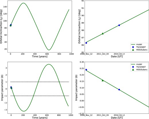
Changes of i_p (upper row) and b (lower row). They are the same types as figure 5. In the left bottom figure, the two black dotted lines show the edges of the stellar disk of WASP-33b. When its impact parameter is between −1 and 1, we are able to see its transit. (Color online)

5 Conclusion

We have conducted Doppler tomographic analyses for WASP-33b using archival J+15 datasets from HJST and a new dataset from Subaru in a homogeneous way. We have modeled WASP-33b’s precession and derived |$i_{\star }=96^{+10}_{-14}$| deg, J₂ = (9.14 ± 0.51) × 10⁻⁵, and the nodal precession timescale to be ∼840 yr. We have estimated that the angle between the line of sight and WASP-33b’s orbital plane oscillates widely with an amplitude of ∼67°, and WASP-33b transits its host star for only ∼20% of the period of its nodal precession.

We point out that nodal precession of hot Jupiters around hot stars should be fairly common, although in varying degrees, since hot stars tend to be oblate due to their rapid rotation and hot Jupiters around hot stars tend to be misaligned. Despite this fact, currently there are only two planets, Kepler-13Ab and WASP-33b, known to show significant nodal precession around A stars. It would also be valuable to measure the nodal precession of another known hot Jupiter, KELT-9b, in the future, because it has a misaligned orbit around a rapidly rotating B/A-type star. Gaudi et al. (2017) indeed guessed that the nodal precession of KELT-9b should be detectable from 2022. In addition, thanks to the ongoing TESS mission, the number of hot Jupiters around B- or A-type stars will increase in the coming years, and more planets suitable for this kind of study will become available. As shown in this paper, measurement of the nodal precession of a hot Jupiter around a hot star can give us useful information about its planetary orbit and its host star, such as the fraction of the period when the planet is transiting in front of the host star compared to the whole precession period, or the stellar gravitational quadrupole moment. Future observations of the nodal precession of hot Jupiters around hot stars will reveal the diversity of those points in detail.

Acknowledgments

This paper is based on data collected at the Subaru Telescope, which is located atop Maunakea and operated by the National Astronomical Observatory of Japan (NAOJ). We wish to recognize and acknowledge the very significant cultural role and reverence that the summit of Maunakea has always had within the indigenous Hawaiian community. The paper includes data taken at The McDonald Observatory of The University of Texas at Austin.

Pyraf is a product of the Space Telescope Science Institute, which is operated by AURA for NASA. This work has made use of the VALD database, operated at Uppsala University, the Institute of Astronomy RAS in Moscow, and the University of Vienna.

This work is partly supported by The Graduate University for Advanced Studies, SOKENDAI, JSPS KAKENHI Grants JP18H01265 and JP18H05439, and JST PRESTO Grant JPMJPR1775.

Appendix. Analytic model of planetary shadow

We adopt an analytic method for a rotational broadening line profile to create a model of a planetary shadow in subsection 2.3. Here we assume that a host star is a solid sphere and its spin axis is normal to the line of sight, though sin i_⋆ ≠ 1. This assumption makes v/V sin i_⋆ equivalent to x, a component perpendicular to the stellar spin axis in units of the stellar radius (see figure 4).

A normalized rotational broadening profile G(x) is given as

$$\begin{eqnarray} G(x)=\frac{G^{^\prime}(x)}{\int ^{\infty }_{-\infty }G^{^\prime }(x) dx} , \end{eqnarray}$$

(A1)

with

$$\begin{eqnarray} G^{^\prime }(x)=\int ^{z_{\mathrm{max}}}_{-z_{\mathrm{min}}}I(x, z) dz, \end{eqnarray}$$

(A2)

where I(x, z) is the stellar surface intensity at (x, z), the projected position relative to the center of the star. When the intensity is a quadratic limb-darkening law,

$$\begin{eqnarray} I(x, z) &=& I_{0}\Bigg[1-u_{1}\big(1-\sqrt{1-x^{2}-z^{2}}\big)\\ &&\,- u_{2}\left(1-\sqrt{1-x^{2}-z^{2}}\right)^{2}\Bigg], \end{eqnarray}$$

(A3)

the rotational broadening line profile becomes

$$\begin{eqnarray} {G^{^\prime }(x)=\left\lbrace \begin{array}{ll}\displaystyle 2(1-u_{1}-u_{2})\sqrt{1-x^{2}}+\frac{\pi }{2}(u_{1}+2u_{2})(1-x^{2})\\\ -\frac{4}{3}u_{2}(1-x^{2})^{3/2} &(|x|<1) \\ 0 &(\mathrm{otherwise}) \end{array} \right.} \\ \end{eqnarray}$$

(A4)

and

$$\begin{eqnarray} \int ^{\infty }_{-\infty }G^{^\prime }(x) dx = \pi \left(1-\frac{u_{1}}{3}-\frac{u_{2}}{6}\right). \end{eqnarray}$$

(A5)

When a planet with radius r(= R_p/R_s) is at (x_p, z_p), the projected position is written as

$$\begin{eqnarray} x_{\rm p}(t)&=&\frac{a}{R_{\rm s}}\sin \left(2\pi \frac{t-T_{0}}{P}\right)\cos \lambda +b\cos \left(2\pi \frac{t-T_{0}}{P}\right)\sin \lambda ,\\ \end{eqnarray}$$

(A6)

$$\begin{eqnarray} z_{\rm p}(t)&=&-\frac{a}{R_{\rm s}}\sin \left(2\pi \frac{t-T_{0}}{P}\right)\sin \lambda +b\cos \left(2\pi \frac{t-T_{0}}{P}\right)\cos \lambda\\ \end{eqnarray}$$

(A7)

with time t and covers the stellar disk, the broadening profile is decreased by

$$\begin{eqnarray} K(x, t) &=& \int ^{z_{2}(x, t)}_{z_{1}(x, t)}I(x, z) dz \\ & =& [1-u_{1}-u_{2}(2-x^{2})](z_{2}-z_{1})+\frac{u_{2}}{3}\big(z^{3}_{2}-z^{3}_{1}\big) \\ && - \frac{u_{1}+2u_{2}}{2}\Bigg \lbrace z_2 \sqrt{1-x^{2}-z^{2}_{2}}-z_1 \sqrt{1-x^{2}-z^{2}_{1}} \\ && +\, (1-x^{2})\left[\sin ^{-1}\left(\frac{z_{2}}{\sqrt{1-x^{2}}}\right)\right.\\ &&\left.-\sin ^{-1}\left(\frac{z_{1}}{\sqrt{1-x^{2}}}\right)\right]\Bigg \rbrace , \end{eqnarray}$$

(A8)

with

$$\begin{eqnarray} {z_{1}=\left\lbrace \begin{array}{ll}0 &\quad \left(|x|>1 \ \mathrm{or} \ |x-x_{\rm p}|>r\right) , \\ \sqrt{1-x^{2}} &\quad \left(z_{\rm p}-\sqrt{r^{2}-(x-x_{\rm p})^{2}} > \sqrt{1-x^{2}}\right) , \\ -\sqrt{1-x^{2}} &\quad \left(z_{\rm p}-\sqrt{r^{2}-(x-x_{\rm p})^{2}} < -\sqrt{1-x^{2}}\right) , \\ z_{\rm p}-\sqrt{r^{2}-(x-x_{\rm p})^{2}} &\quad (\mathrm{otherwise}) \end{array} \right.} \end{eqnarray}$$

(A9)

and

$$\begin{eqnarray} {z_{2}=\left\lbrace \begin{array}{ll}0 &\quad \left(|x|>1 \ \mathrm{or} \ |x-x_{\rm p}|>r\right) , \\ \sqrt{1-x^{2}} &\quad \left(z_{\rm p}+\sqrt{r^{2}-(x-x_{\rm p})^{2}} > \sqrt{1-x^{2}}\right) , \\ -\sqrt{1-x^{2}} &\quad \left(z_{\rm p}+\sqrt{r^{2}-(x-x_{\rm p})^{2}} < -\sqrt{1-x^{2}}\right) , \\ z_{\rm p}+\sqrt{r^{2}-(x-x_{\rm p})^{2}} &\quad (\mathrm{otherwise}) . \end{array} \right.} \end{eqnarray}$$

(A10)

The convolution between K(x, t) and the stellar intrinsic Gaussian profile is our model of the planetary shadow.

Finally, we note that in the appendix of Hartman et al. (2015), part of the above expression,

$$\begin{eqnarray} z_{2}\sqrt{1-x^{2}-z_{2}^{2}}-z_{1}\sqrt{1-x^{2}-z_{1}^{2}}, \end{eqnarray}$$

(A11)

in equation (A8) appears to be mistakenly expressed as

$$\begin{eqnarray} z_{2}\big(1-x^{2}-z_{2}^{2}\big)-z_{1}\big(1-x^{2}-z_{1}^{2}\big). \end{eqnarray}$$

(A12)

References

Abt

H. A.

,

Levato

H.

,

Grosso

M.

2002

,

ApJ

,

573

,

359

Collier Cameron

A.

et al. .

2007

,

MNRAS

,

375

,

951

Collier Cameron

A.

et al. .

2010

,

MNRAS

,

407

,

507

Donati

J.-F.

,

Semel

M.

,

Carter

B. D.

,

Rees

D. E.

,

Collier Cameron

A.

1997

,

MNRAS

,

291

,

658

Eastman

J.

,

Siverd

R.

,

Gaudi

B. S.

2010

,

PASP

,

122

,

935

Foreman-Mackey

D.

2016

,

J. Open Source Software

,

1

,

24

Foreman-Mackey

D.

,

Hogg

D. W.

,

Lang

D.

,

Goodman

J.

2013

,

PASP

,

125

,

306

Gaudi

B. S.

et al. .

2017

,

Nature

,

546

,

514

PubMed

Hartman

J. D.

et al. .

2015

,

AJ

,

150

,

197

Herman

M. K.

,

de Mooij

E. J. W.

,

Huang

C. X.

,

Jayawardhana

R.

2018

,

AJ

,

155

,

13

Husser

T.-O.

,

Wende-von Berg

S.

,

Dreizler

S.

,

Homeier

D.

,

Reiners

A.

,

Barman

T.

,

Hauschildt

P. H.

2013

,

A&A

,

553

,

A6

Iorio

L.

2011

,

Ap&SS

,

331

,

485

Iorio

L.

2016

,

MNRAS

,

455

,

207

Johnson

M. C.

et al. .

2018

,

AJ

,

155

,

100

Johnson

M. C.

,

Cochran

W. D.

,

Collier Cameron

A.

,

Bayliss

D.

2015

, ApJ, 810, L23

(J+15)

Kipping

D. M.

2013

,

MNRAS

,

435

,

2152

Kochukhov

O.

,

Makaganiuk

V.

,

Piskunov

N.

2010

,

A&A

,

524

,

A5

Kovács

G.

et al. .

2013

,

A&A

,

553

,

A44

Kupka

F. G.

,

Ryabchikova

T. A.

,

Piskunov

N. E.

,

Stempels

H. C.

,

Weiss

W. W.

2000

,

Baltic Astron.

,

9

,

590

Lehmann

H.

,

Guenther

E.

,

Sebastian

D.

,

Döllinger

M.

,

Hartmann

M.

,

Mkrtichian

D. E.

2015

,

A&A

,

578

,

L4

Noguchi

K.

et al. .

2002

,

PASJ

,

54

,

855

Parviainen

H.

,

Aigrain

S.

2015

,

MNRAS

,

453

,

3821

Pepper

J.

et al. .

2007

,

PASP

,

119

,

923

Tull

R. G.

,

MacQueen

P. J.

,

Sneden

C.

,

Lambert

D. L.

1995

,

PASP

,

107

,

251

von Essen

C.

et al. .

2014

,

A&A

,

561

,

A48

von Essen

C.

,

Mallonn

M.

,

Welbanks

L.

,

Madhusudhan

N.

,

Pinhas

A.

,

Bouy

H.

,

Weis Hansen

P.

2019

,

A&A

,

622

,

A71

Wright

J. T.

,

Eastman

J. D.

2014

,

PASP

,

126

,

838