


Abstract
On 2011 March 7, the Solar Neutron Telescope located at Mt. Sierra Negra, Mexico (4600 m) observed enhancements of the counting rate from 19:57 to 20:04 UT with statistical significance 6.8σ and from 20:36 to 21:03 UT with 5.8σ. One plausible physical explanation for the observation enhancements is that they were produced by solar gamma-rays. The intensities were estimated to be (0.16 ± 0.03) photons cm−2 s−1 for the first flare and (0.22 ± 0.04) photons cm−2 s−1 for the second one at the top of the atmosphere. As far as we know, this is the first report on the detection of solar gamma-rays with a ground-based detector. In association with these events, the solar neutron detector Space Environment Data Acquisition Equipment on board the International Space Station registered two solar neutrons with statistical significances of 7.3σ and 6.6σ. The Large Area Telescope on board the Fermi observatory also observed high-energy gamma-rays from this flare with a statistical significance of 6.7σ. In this paper we propose a unified model to explain the production mechanism of high-energy gamma-rays and neutrons in association with this flare.
1 Introduction
The solar flare observed at 19:48 UT on 2011 March 7 may be one of the most important flares observed in Solar Cycle 24. Hereafter, we refer to it as the SOL2011-03-07 flare. Although the X-ray intensity of the flare measured with the GOES satellite was of a moderate scale, M3.7, the event has already provided us with important information: emission of long-lasting, high-energy gamma-rays that were detected with the Large Area Telescope on board the Fermi satellite (FERMI-LAT). This emission continued for almost 14 hr and high-energy gamma-rays with an energy of ∼4 GeV were recorded with a statistical significance of 6.7σ (Ackermann et al. 2014). Another relevant fact is that this marked the first detection of solar neutrons in Solar Cycle 24 with the solar neutron telescope (SEDA-FIB) on board the International Space Station (ISS; Koga et al. 2017). Complementary to these observations, the Solar Neutron Telescope (SNT) located at Mt. Sierra Negra in Mexico registered two enhancements of the counting rate during the flare (Muraki et al. 2013). The Mt. Sierra Negra observatory is located at an altitude of 4600 m above sea level.
In this paper we discuss whether these observations may be explained by a unified model. The paper is organized as follows: the next section introduces a general view of the SOL2011-03-07 flare observed with various space instruments. Sections 3 and 4 provide details of the data and the SNT detector. In sections 5 and 6, SNT data are compared with data from SEDA-FIB and FERMI-LAT. In section 7 we propose a unified model which may explain that the observed fluxes are high-energy gamma-rays and neutrons. In section 8 we summarize the results. In appendix 1, as further evidence, we introduce another candidate observation of high-energy gamma-rays observed with the SNT located in Tibet in association with the flare of SOL2011-09-25.
2 General view of the SOL2011-03-07 flare
We present here the space environment data obtained from 19:30 to 21:00 UT on 2011 March 7. The data are from five different satellites and one ground-based detector: GOES, RHESSI (Lin et al 2002), FERMI-GBM (Meegan et al. 2009), FERMI-LAT (Atwood et al. 2009), and SEDA-FIB, as well as the SNT at Mt. Sierra Negra, Mexico (Valdes-Galicia et al. 2004). Figure 1 presents the time profiles of these data. The following subsections provide a description of the data observed with each detector.
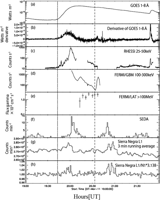
Counting rates of the five detectors from 19:00 to 22:00 UT of the SOL2011-03-07 event. From top to bottom: (a) X-ray intensity curve measured with the GOES at wavelengths of 1–8 Å; (b) differential time profile of the GOES X-ray intensity; (c) hard X-ray intensity curve measured by RHESSI in the 25–50 keV region; (d) hard X-ray time profile measured with FERMI-GBM in the 100–300 keV region; (e) gamma-ray time profile measured with FERMI-LAT for photons with Eγ > 100 MeV; (f) counting rate of the SEDA neutron detector for neutrons with En > 35 MeV; (g) Sierra Negra SNT counting rate of the L1 channel (three-minute running average data); and (h) Sierra Negra SNT counting rate of the L1 channel normalized by the N1 channel by multiplying by a factor of 3.138.
2.1 GOES data
Figures 1a and 1b show the GOES 1–8 Å data and the GOES time derivative. The soft X-ray sensors on the GOES satellite detected a flare that started at 19:43 UT and reached its maximum at 20:12 UT with a magnitude of M3.7. The flare position is listed at N23° W50° on the solar surface in Active Region 1164 (GOES data 2011).1
2.2 RHESSI satellite
Figure 1c shows the Reuven Ramaty High Energy Solar Spectroscopic Imager (RHESSI) event rates at 25–50 keV (see RHESSI web site).2 RHESSI observed this flare from 19:27 to 20:08 UT. The emission of hard X-rays at 25–300 keV started at ∼19:47 UT and peaked at 20:00 UT. Two-dimensional images were made for the times of maxima at 19:57 UT and 20:01 UT. The peak positions of hard X-rays and soft gamma-rays are estimated using the RHESSI data at the heliocentric coordinates (625″, 560″) for 19:57 UT and (610″, 560″) for 20:01 UT, respectively, and these coordinates correspond to the flare position indicated above (Muraki et al. 2013).
2.3 FERMI-GBM results
FERMI involves two main detectors (GBM and LAT). The Gamma-ray Burst Monitor (GBM) detects gamma-ray bursts in the X-ray range from 6 to 300 keV (Meegan et al. 2009). FERMI-GBM observed the Sun from 20:02 to 20:40 UT on 2011 March 7. The intensity of hard X-rays in the range 100–300 keV was 2000 counts s−1 at 20:02 UT. As shown in figure 1d, the count rate profile shows that the maximum was seen with FERMI-GBM shortly before the observation started: on the third peak at 20:38 UT, a counting rate of ∼800 counts s−1 was recorded. Unfortunately, both GBM and LAT failed to observe the rising phase of the impulsive peak seen with RHESSI.
2.4 FERMI-LAT results
The high-energy gamma-ray detector FERMI-LAT observed the flare from 20:15 to 20:40 UT. The time profile is given in figure 1e (Share et al. 2018). The emission of gamma-rays continued for 14 hr beyond this time. High-energy gamma-rays with a peak intensity at 200 MeV were detected. The details were published in Ackermann et al. (2014). However, once again we stress here that FERMI-LAT did not observe the impulsive phase of the flare. Therefore, we could not directly compare the FERMI-LAT data with the data of SNT that were recorded at the impulsive phase. In section 7, we construct a unified model that is able to explain the production process of these high-energy gamma-rays.
2.5 SEDA-FIB results on the ISS
The SEDA-FIB (scintillation FIBer detector) is a neutron sensor on board the ISS. The sensor can measure the energy and arrival direction of neutrons. Details may be found in Imaida et al. (1999), Koga et al. (2011), and Muraki et al. (2012). The production time may be estimated using information on the energy of neutron-induced protons in the sensor. Figure 1f shows the time profile of solar neutrons. However, SEDA-FIB failed to detect the high-energy neutrons possibly produced in the impulsive phase of the first peak. This is because the ISS stayed over the night area of the Earth until 20:02 UT. Therefore, neutrons may possibly have arrived between 19:58 and 20:02 UT, but could not be detected. The energy of these neutrons is higher than 300 MeV.
2.6 SDO satellite
The Solar Dynamics Observatory (SDO) also observes the Sun by means of ultraviolet telescopes over different wavelengths (Lemen et al 2012). The SDO satellite observed the emission of a coronal mass ejection (CME) associated with this flare from the start time of the emissions (Cheng et al. 2013). Thus, the satellite observed not only the start of the CME but also its development from the beginning of the impulsive flare at ∼19:47 UT (Share et al. 2018); the ejection measured 2125 km s−1 in speed during 20:00–22:30 UT (SOHO LASCO CME Catalog).3
2.7 SNT at Mt. Sierra Negra (SN-SNT)
The Solar Neutron Telescope consists of plastic scintillators surrounded by proportional counters (PC) in anti-coincidence, to separate the flux of neutral particles from charged particles. Figure 1g shows the time profile of the L1 channel between 19:00 and 21:30 UT as observed with SN-SNT. The L1 channel measures the flux of neutral particles (n or γ) crossing the scintillator and triggering the PC underneath (Valdes-Galicia et al. 2004). Two clear enhancements from 19:49 to 20:02 UT and from 20:50 to 21:02 UT may be recognized. Figure 1h shows the ratio between the two counting rates: the L1 channel divided by the N1 channel. Detailed explanations of the L1 and N1 channels are provided in the next section, together with their detection efficiency estimated by a Monte Carlo simulation.
3 Detection principle for gamma-rays and neutrons with the SNT
Figure 2 shows a schematic diagram of the SNT at Mt. Sierra Negra. The detector has a central scintillator and proportional counter gondolas covering the five surfaces surrounding the scintillator. A lead plate with a thickness of 5 mm was set on top of the detector. The scintillator is 30 cm thick and has a total surface area of 4 m2.
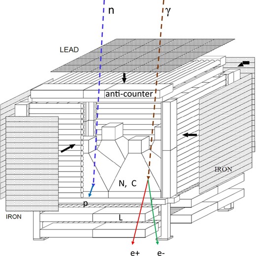
Schematic diagram of the Mt. Sierra Negra Solar Neutron Telescope located at 4600 m. The N signals are produced by the central scintillator without any signal in the anti-counter, while the signals of charged particles C are created by the coincidence between the signals induced by the central scintillator (N) and the signals recorded by the anti-counter. The L signals are formed by the coincidence between the N1 signals and those deposited in the proportional counters underneath the scintillator. Diagrams of the detection principle of neutrons (left) and gamma-rays (right) using the L detectors are also presented. (Color online)
The detector is operated under the following principles: (1) the discrimination of charged particles from neutral ones, for which the gondolas of the PCs at the top and four sides of the telescope are used as an anti-coincidence system; (2) conversion of neutral particles to charged ones inside the thick plastic scintillator located at the central part of the SNT; and (3) tracking the arrival directions of incoming particles due to the coincidence grid constructed with the four layers of PCs underneath the plastic scintillators. For this purpose, the layers are alternatively set at right angles to each other, as shown in figure 2. These four layers of PCs are labeled L1 to L4 from top to bottom. Here, L stands for the lower layer under the plastic scintillator.
3.1 Definition of each channel and selection performance between n and γ
The signals observed in the Neutral channel (N) of the central plastic scintillator are labeled N1–N4, depending on the threshold energy of each channel (30, 60, 90, and 120 MeV). The signals of the L1–L4 channels are produced with the coincidence of the N1 channel. And C represents the counting rate of the central plastic scintillator produced by charged particles, such as e, p, and μ.
Neutrons and gamma-rays penetrate the anti-coincidence counter system. Neutrons experience nuclear interactions with the hydrogen and carbon nuclei in the plastic scintillator, producing protons that may be detected. Gamma-rays also deposit signals in the plastic scintillator when making electromagnetic interactions with the electric field of the nuclei inside the plastic scintillator. Therefore, incoming gamma-rays are converted into electron–positron pairs in the scintillator (as depicted on the right-hand side of figure 2). Among the electrons and positrons produced, those reaching energies in excess of 30 MeV (i.e., the threshold energy of the scintillators) produce a signal above the discriminator. These are the minimum-ionizing particles that just penetrate the scintillator and arrive at the lower layers.
Conversely, protons converted from neutrons lose more energy inside the scintillator as compared with electrons and positrons. Thus, they often stop inside the scintillator (as depicted on the left-hand side of figure 2). Only high-energy protons penetrate the scintillator and arrive at the lower proportional counters. Therefore, as explained in the next section, the excess of the L1–L4 channels seen during flare SOL2011-03-07 suggests that the observed increases could possibly be induced by gamma-rays. In other words, higher counting rates of the lower proportional counters (L1–L4) during a solar flare suggests the arrival of gamma-rays or high-energy neutrons (En > 1 GeV) in association with the respective flare. The above statements were confirmed by a Monte Carlo simulation.
3.2 Response function of each channel
The response functions of each N and L channel to particles arriving at the detector are shown in figure 3 as a function of incident energy. There are three remarkable differences in the detection efficiency between neutrons and gamma-rays: (1) the rapid rise of the detection efficiency at the threshold energy for gamma-rays, while it rises more gradually for neutrons; (2) a similar detection efficiency of the N1–N4 channels for both neutrons and gamma-rays around ∼300 MeV; and (3) about one order higher detection efficiency for gamma-rays of the L1–L4 channels at Eγ ∼ 100 MeV in comparison with that of neutrons at the same energies.
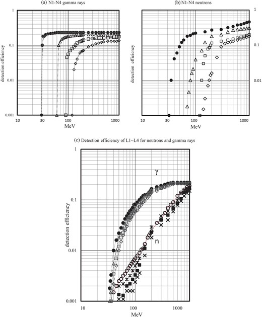
Detection efficiency of incoming neutrons and photons of each channel is presented as a function of the incident energy. (a) Response curves of the SNT at Mt. Sierra Negra for gamma-rays. (b) Response curve of the SNT for incident neutrons. (c) Response curve of L1–L4 channels for neutrons and gamma-rays. The upper black labels N1(•), N2(Δ), N3(|$\square $|), and N4(◊) indicate the detection efficiency of the neutral channels of the thick plastic scintillator, while the lower symbols of L1(|$\circ $|), L2(*), L3(▪), and L4 (×) represent the detection efficiency for the lower arrays located under the central thick plastic scintillator, composed of PCs with the coincidence of the N1 signal. The black solid circle corresponds to gamma-rays, while the open circle represents the detection efficiency of neutrons of the L1 channel. (Color online)
Therefore, as explained in the next section, the excess of the L1–L4 channels suggests that the observed increases could possibly be induced by gamma-rays. In other words, higher counting rates of the lower PCs (L1–L4) during a solar flare may suggest either the arrival of gamma-rays or high-energy neutrons (En > 1 GeV) in association with the respective flare.
Figure 3c indicates the relative detection efficiencies for gamma-rays and neutrons. When the incident energy of neutrons and gamma-rays approaches 1 GeV, the reduction of the separation ability may be predicted. However, this may not actually happen. Because the production spectrum of high-energy gamma-rays and neutrons is expected to be less intense at higher energies (typically ∼1000 times less intensive between En,γ = 100 MeV and 1000 MeV for a power-law spectrum index of 3). Another limitation is the different fragmentation process of the energies of gamma-rays and neutrons when they propagate in the atmosphere (see appendix 2).
Table 1 gives details of the threshold energy for each channel, along with the typical counting rates. The energy calibration for each channel was performed using relativistic muons passing through the detector from top to bottom. A more complete description of the SN-SNT may be found in Valdes-Galicia et al. (2004).
Counting rate of each channel of the SNT.*
| Observation point | Mt. Sierra Negra |
|---|---|
| Altitude | 4580 m |
| Vertical atmospheric pressure | 575 g cm−2 |
| Geophysical coordinates | N|$19^{\circ}0'$|, W|$97^{\circ}3'$| |
| Sensor surface area | 4.0 m2 |
| Sensor thickness | 30 cm |
| Interaction probability for n | 0.307 |
| Pair-creation probability for γ | 0.208 |
| Counting rate C1 (min−1) | 173000 (> 30 MeV) |
| Counting rate C2 | 77600 (> 60 MeV) |
| Counting rate C3 | 30100 (> 90 MeV) |
| Counting rate C4 | 14600 (> 120 MeV) |
| Counting rate N1 (min−1) | 86400 (> 30 MeV) |
| Counting rate N2 | 32500 (> 60 MeV) |
| Counting rate N3 | 10080 (> 90 MeV) |
| Counting rate N4 | 4880 (> 120 MeV) |
| Counting rate L1 (min−1) | 27500 |
| Counting rate L2 | 16130 |
| Counting rate L3 | 12400 |
| Counting rate L4 | 9240 |
*Parameters and typical counting rates of the neutron telescopes of Mt. Sierra Negra. In the table, the interaction probabilities for n and pair creation for γ do not include the threshold effect due to the discriminator. The interaction probability is given for neutrons with an energy of ∼20 GeV. In the case of solar neutron detection at about ∼500 MeV, the value would be slightly higher than this value at ∼0.46.
4 Data recorded by the SNT
Figure 4 presents the detailed counting rates of the N1 and L1 channels of the SNT observed in the SOL2011-03-07 flare. The solid line represents the time profile of the N1 channel and the red dashed line corresponds to the L1 channel. The counting rate of the LI channel is multiplied by a factor of 3.138 to give a similar counting rate level in both channels. Clear excesses may be recognized around ∼19:58 UT and ∼20:50 UT in the L1 rate. The continuous black dashed line represents the smoothed rate in the N1 channel. We regarded this line as the background line for the L1 channel. The deviations from the dashed line are regarded as an excess or decrement of the L1 channel. (The excess or decrement at the time t is defined as |${\rm{\Delta }}I( t ) = I( t ) - \langle {I( {{t_i}} )} \rangle $|, where |$\langle {I( {{t_i}} )} \rangle $| represents the average counting rate around ti.) We have calculated the statistical significances of the excesses during two time intervals: 19:48–20:04 UT and 20:45–21:04 UT, as indicated by the vertical green lines in figure 4. The significances of these excesses are estimated to be 8.0σ and 12.9σ, respectively. These statistical significances are quite high; therefore, it would be quite hard to attribute the excesses to chance coincidence. The statistical significances are derived by a simple formula |$( {\Delta I/\sqrt N } )$|, i.e., |$5471/686{\rm{\ }} = {\rm{\ }}8.0{\rm{\ }}$|and |$9544/740{\rm{\ }} = {\rm{\ }}12.9$| for the two intervals.
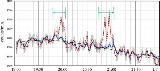
Counting rates for one-minute periods of the SN-SNT between 19:00 and 22:00 UT for the SOL2011-03-07 event. The black solid line represents the counting rate of the N1 channel, while the red dashed curve shows the counting rate of the L1 channel. To compare both counting rates, the counting rate of the L1 channel is multiplied by a factor of 3.138. The definition of the N and L channels are given in the text. The vertical bar represents the statistical error of each point. The black dashed curve corresponds to the best-fitting curve to the N1 count by the third-order polynomial function |$y\ = {\rm{\ }}212.11{x^3} - 13287{x^2} + 276410x - 1823533$|, where y represents the counting rate for one minute, while x corresponds to the time in units of hours (UT). The vertical green lines delimit the times of the two significant increases. (Color online)
Figure 5 shows a plot made to compare the present enhancements with a solar-neutron event observed with the same detector on 2005 September 7 (SOL2005-09-07). From left to right, each point represents the excess of the counting rate of the N1–N4 channels (ΔNi, i = 1–4) and L1–L4 channels (ΔLi, i = 1–4) of SN-SNT (normalized to ΔN1).
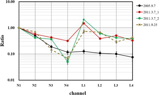
One-minute-value excess registered by the N and L channels, normalized to the excess of the N1 channel (ΔN1). The red line indicates the first peak of the SOL2011-03-07 event; the green line indicates the second peak. The brown dashed curve presents the excess ratio of the counting rate recorded by the Yangbajing SNT for SOL2011-09-25 (details are given in appendix 1). These three plots have a remarkable difference compared with the counting rates recorded by the solar neutron event registered on SOL2005-09-07. The excesses of the L1–L4 channels are easily recognized. (Color online)
In the solar-neutron event observed with the same detector in the SOL2005-09-07 event (Sako et al. 2006), the excess of the L1–L4 channels (ΔLi) was much less than that of the N1 channel (ΔN1), and gradually decreased from N1 to L4. That is the expected behavior for neutrons. But for the excess observed in the case of SOL2011-03-07, the excesses of the L1–L4 channels were comparatively much higher than those of the SOL2005-09-07 event. Therefore, as described in the previous section, the excess of the counting rate of the L1–L4 channels (ΔLi) could be an indication of the arrival of high-energy gamma-rays in association with the SOL2011-03-07 event. Figure 5 also includes the corresponding data for SOL2011-09-25 registered by the Yangbajing SNT (the brown dashed curve). The details are discussed in appendix 1.
Table 1 lists the values used to estimate the excess flux of every channel at the peak time per minute and per unit area. For the first and second peaks of the L1 channel, the values are (201 ± 7) counts m−2 min−1, and (296 ± 9) counts m−2 min−1, respectively. Estimates of the excess of the N1 channel counting rates give (43 ± 3) counts m−2 min−1 and (70 ± 4) counts m−2 min−1 for the corresponding first and second peaks of the N1 channel, respectively. The two peak times were observed at 19:57–19:58 UT and 20:55–20:56 UT respectively. Table 2 summarizes these values.
Statistical significance of relevant channels for each event registered.*
| Observatory | Sierra Negra | |
|---|---|---|
| Excess time | 19:57–20:04 UT | 20:36–21:03 UT |
| Statistical significance: L1 | 6.8σ >30 MeV† | 5.8σ >30 MeV‡ |
| Statistical significance: N1 | 3.0σ >30 MeV | 2.3σ >30 MeV |
| Excess of L1 channel | 201 ± 7 events min−1 m−2 | 296 ± 9 events min−1 m−2 |
| Excess of N1 channel | 43 ± 3 events min−1 m−2 | 70 ± 4 events min−1 m−2 |
| Air thickness to the Sun | 670 g cm−2 | 777 g cm−2 |
| Zenith angle to the Sun | 31|${^{\circ}_{.}}$|3 | 42|${^{\circ}_{.}}$|3 |
| Comments | First peak | Second peak |
| Observation day | 2011 March 7 | |
*Statistical significances of the excesses for each peak in the SN-SNT L1 and N1 rates. The excess count rates of the L1 and N1 channels at the peak time are given per unit area (m−2) and per unit time (min−1) in rows 5 and 6.
†The statistical significance was given during the eight minutes from 19:57 UT to 20:04 UT. The excesses of the one-minute value are estimated to be 5.8σ (at 19:58 UT) and 6.5σ (at 20:07 UT).
‡The start time of high-energy gamma-ray emission for the second SN-SNT peak was selected at 20:33 UT, when FERMI-GBM detected the start of a second peak in the soft gamma-ray emission.
To convert the observed excess of the N1 channel (ΔN1) to the flux of gamma-rays at the top of the detector, we divide the ΔN1 value by the detection efficiency of the central plastic scintillator. The detection efficiency of each channel is given in figure 3, estimated by a Monte Carlo simulation. A numerical estimate based on the simulation is given in table 3. Taking into account the energy dependence of the counting rate between the N1 and L1 channels (as shown in figure 3), we derived the flux at the top of the atmosphere from the N1 channel data (ΔN1). They were (0.14 ± 0.03) counts cm−2 s−1 and (0.22 ± 0.04) counts cm−2 s−1 for the first and second peaks, respectively.
Gamma-ray flux at the top of the atmosphere.*
| Event date | 2011 March 7 (first) | 2011 March 7 (second) |
|---|---|---|
| Observatory | Sierra Negra | Sierra Negra |
| Detection efficiency of γ by Monte Carlo simulation | 0.21 ± 0.01 (Eγ > 30 MeV) | 0.21 ± 0.01 (Eγ> 30 MeV) |
| Gamma-ray flux at the top of the mountain detector | 206 ± 30 counts m−2 min−1 | 333 ± 33 counts m−2 min−1 |
| Predicted 1 GeV photon flux at the top of the atmosphere (count m−2 min−1) | 0.064 for γ = 50.29 for γ = 4.51.2 for γ = 410.5 for γ = 3 | 0.93 for γ = 54 for γ = 4.516 for γ = 483 for γ = 3 |
| Predicted photon flux at the top of the atmosphere (count m−2 min−1) | (8.3 ± 1.7) × 104 (γ = 3–5)Eγ> 100 MeV | (1.35 ± 0.22) × 105 (γ = 3–5) Eγ> 100 MeV |
| (counts cm−2 s−1) | 0.14 ± 0.03 | 0.22 ± 0.04 |
| E γ > 100 MeV | E γ > 100 MeV | |
| Atmospheric thickness toward the Sun | 670 g cm−2 | 777 g cm−2 |
*Flux of gamma-rays at the top of the atmosphere estimated from the observed photon flux at the peak time with the ground detector. The detection efficiency for gamma-rays referred to in this table was obtained from the Monte Carlo simulation, taking into account the threshold energy on each channel. The threshold energy of the scintillator is Eγ > 30 MeV. The error bars of rows 11 and 14 correspond to the errors arising from the uncertainty of the power index γ = 3–5 of the initial gamma-rays.
5 Solar neutrons observed with SEDA-FIB
5.1 Neutron events detected with SEDA-FIB in the SOL2011-03-07 flare
Here we discuss the neutron production in association with the M3.7 SOL2011-03-07 flare. The SEDA-FIB neutron detector on board the ISS observed excesses of neutrons from this flare. SEDA-FIB is a detector that can measure the arrival direction and energy of incoming neutrons and that collects neutrons with energy higher than 35 MeV. The SEDA-FIB sensor provides directional information, and tracks of neutrons within 45° of the cone from the solar direction were selected as solar origin candidates. Imaida et al. (1999), Koga et al. (2011), and Muraki et al. (2012, 2017) provide details about the detector and related processes.
An estimate of the neutron-induced-proton energy in the sensor may be used for calculating the production time of solar neutrons. Based on this estimate, with the additional assumption of an instantaneous production of neutrons in the SOL2011-03-07 event, we could reproduce an energy spectrum for solar neutrons. Judging from the time profiles of hard X-rays in the RHESSI satellite and FERMI-GBM satellite (see figures 1c and 1d), the most likely times for solar neutron production were assumed at approximately 19:58 UT (for the first peak) and 20:37 UT (for the second peak). Figure 6 indicates these points with arrows. At 19:58 UT, the RHESSI channel of 25–50 keV observed a rapid increase in intensity (see figure 1c). Then at 20:37 UT, the hard X-ray detector of FERMI-GBM detected a peak flux of X-rays in the 100–300 keV energy band (see figure 1d). Therefore, we assumed the production times of neutrons at 19:58 UT and 20:37 UT, and obtained the energy spectra by applying the time-of-flight method to the observed neutrons.
![Counting rate of SEDA-FIB between 19:00 and 22:00 UT of the SOL2011-03-07 event, together with the GOES differential flux. The ISS passed through the night region during 19:32–20:02 UT and 21:02–21:32 UT, as indicated by the black bar underneath the abscissa. The horizontal axis is presented in units of minutes, starting at 19:00 UT. The red diamonds represent neutrons coming from the solar direction. The brown dashed curve is the empirical curve for the inseparable background that may be described by the function $3{\rm{*si}}{{\rm{n}}^4}[ {\pi ( {t - {t_0}} )/45} ].$ Details of the parameters are given in the text. There is a factor of about 10 between the green and brown dashed curves due to the selection of the solar-directed neutrons. The main background neutrons are coming from the direction of the pressurized vessel of the ISS. These neutrons are produced by cosmic rays colliding with the main ISS body. The scale is arbitrary for the GOES differential intensity. The exact scale is presented in figure 1b. The arrows indicate the peak points of hard X-rays in the energy band of 100–300 keV for the first peak and the second peak seen with FERMI-GBM. The high-intensity peak of the GOES data point at 21:45 UT was produced by a different M1.5 flare in the region of 1165. (Color online)](https://oup.silverchair-cdn.com/oup/backfile/Content_public/Journal/pasj/72/2/10.1093_pasj_psz141/2/m_pasj_72_2_18_f8.jpeg?Expires=1749459440&Signature=TkcFVT3suBDiqaAeD6z2gS7EDLcb8xEcEhOzqK7TDsZTjhU2ww9iCHBf7zJbvXSOcwB8PeRYAvyxZKV790fGObAOfEqYWhnVSlMl-qtIVX98ZQuUbS4dC8FxYS1rf92354Bgba4B9tOx7DjPoxWI7DBV9KvntD4wWLXWigsbMWBmniFAtfiskr5~zbgyI1SUxQ-y1C8CDhgOPDo4Wgb-k49N9ejCO96j7vHKmDjjLGiHD4OA-eCvCnFghkhmm2SYD7jjb8zpLZKUEeUD0QVvyW9P6b8fNIIF6QLsw5HhvhIfMiFKLdo2N63HaPaTPLkm-vDMaV-UTI2Usaf3K7tBrw__&Key-Pair-Id=APKAIE5G5CRDK6RD3PGA)
Counting rate of SEDA-FIB between 19:00 and 22:00 UT of the SOL2011-03-07 event, together with the GOES differential flux. The ISS passed through the night region during 19:32–20:02 UT and 21:02–21:32 UT, as indicated by the black bar underneath the abscissa. The horizontal axis is presented in units of minutes, starting at 19:00 UT. The red diamonds represent neutrons coming from the solar direction. The brown dashed curve is the empirical curve for the inseparable background that may be described by the function |$3{\rm{*si}}{{\rm{n}}^4}[ {\pi ( {t - {t_0}} )/45} ].$| Details of the parameters are given in the text. There is a factor of about 10 between the green and brown dashed curves due to the selection of the solar-directed neutrons. The main background neutrons are coming from the direction of the pressurized vessel of the ISS. These neutrons are produced by cosmic rays colliding with the main ISS body. The scale is arbitrary for the GOES differential intensity. The exact scale is presented in figure 1b. The arrows indicate the peak points of hard X-rays in the energy band of 100–300 keV for the first peak and the second peak seen with FERMI-GBM. The high-intensity peak of the GOES data point at 21:45 UT was produced by a different M1.5 flare in the region of 1165. (Color online)
Figure 6 shows the counting rate of the SEDA-FIB detector during four orbits of the ISS. The red diamonds correspond to the solar neutron candidates. The green dashed curve presents an empirical curve for the counting rate expressed by |$( {{A_1}} ) \times {\rm{\ si}}{{\rm{n}}^4}[ {\pi ( {t - {t_0}} )/45} ] + 3$|, where t represents the time from time t0 in units of minutes. We took A1 = 27 and t0 = 0 at 19:00 UT for figure 6. The ISS was in the night region from 19:32 to 20:02 UT and from 21:02 to 21:32 UT, as indicated by the black horizontal line under figure 6. The brown dashed curve represents the approximate curve for neutrons arriving from the solar direction as expressed by |$( {{A_2}} ) \times {\rm{\ si}}{{\rm{n}}^4}[ {\pi ( {t - {t_0}} )/45} ]$|, where A2 = 3. Selecting only solar-directed neutrons within 45° of the Sun reduces the background neutrons by a factor of about 10 when we compare the brown dashed curve with the green dashed ones. The omnidirectional background neutrons mainly come from the interactions of cosmic rays with the ISS body.
We regard the brown dashed curve as the solar background and we subtracted the counts from the data. The remaining events are regarded as solar neutrons. The total numbers of solar neutrons are estimated to be 51 and 21 events for the respective peaks. The statistical significances are 7.3σ (for the excess during the 9 min) and 6.6σ (for the excess during the 5 min) respectively. We then created the energy spectrum associated with these events. Figures 7a and 7b show the energy spectra for the first peak and second peak respectively, based on the assumption of an instantaneous production of neutrons at 19:58 UT and 20:37 UT, respectively.
Solar neutron energy spectra for (a) the first and (b) the second bumps observed by the SEDA-FIB detector. Instantaneous production of neutrons on the solar surface was assumed. We assumed that neutrons were produced at the hard X- ray maxima times of 19:58 UT (a) and 20:37 UT (b). The gray diamonds denote the observed data; the black squares denote the data corrected for the decay effect in flight between the Sun and Earth.
5.2 Neutron flux measured by SEDA-FIB
To derive the neutron flux of the first peak detected by SEDA-FIB in association with the SOL2011-03-07 flare, the flux corresponding to neutrons with En > 100 MeV is calculated as follows: from figure 7a (left side), the number of neutrons after the correction due to decay during flight between the Sun and Earth should be (132 ± 18) neutrons (100 cm)−2 (or 13200 ± 1800 m−2). Taking into account the neutron detection efficiency of the SEDA-FIB detector, estimated to be (1.8% ± 0.5%) (Muraki et al. 2016), the neutron flux at the top of the atmosphere is (73 ± 10 ± 22) neutrons cm−2 for En > 100 MeV. The first error arises from statistical fluctuation, while the second error stems from the energy dependence of the neutron conversion factor in the detector. Later we use this value and compare it with the intensity of gamma-rays measured by the SNT located at Mt. Sierra Negra.
For the second peak, the solar neutron flux with energy higher than 50 MeV is calculated as follows. After correction for the decay in flight, the flux of neutrons is estimated to be (134 ± 25) neutrons (100 cm)−2 (= 13400 ± 2500 m−2; see figure 7b, right side). Considering the detection efficiency of SEDA-FIB in detecting neutrons (1.8% ± 0.5%), the flux of solar neutrons at the top of the atmosphere is estimated to be (75 ± 14 ± 22) neutrons cm−2 for En > 50 MeV. The first and second errors correspond to the statistical error and the energy conversion one, respectively. Combining the two errors, the flux is estimated to be (73 ± 24) neutrons cm−2 for En > 100 MeV for the first peak and (75 ± 26) neutrons cm−2 for En > 50 MeV for the second peak.
6 Comparison of neutron and gamma-ray results
Now we compare the excess rates measured by the ground-based detector SN-SNT in the impulsive phase with the neutron rates observed in space at the same time, assuming that they are from gamma-rays. For this purpose, we need to convert the fluxes measured by the ground-based detector to gamma-ray intensities at the top of the atmosphere.
Gamma-rays are attenuated in the atmosphere. However, some gamma-rays arrive at the detectors located on high mountains under low atmospheric pressure without absorption. We need to know the average number of gamma-rays penetrating the detector for the specific atmospheric depth as a function of the incident energy of gamma-rays. To perform that calculation we did Monte Carlo simulations based on GEANT4. The details of the simulation processes are given in appendix 2.
At the first peak of the SOL2011-03-07 flare, the assumed gamma-rays and neutrons were both detected at the same time. Therefore, we may compare the two fluxes. With that purpose, we derive the ratio between the fluxes of neutrons and gamma-rays as a function of the spectral power-law index of the primary ions accelerated during the flare. We may then compare the predicted |$n/{\rm{\gamma }}$| ratio with the observed ratio.
6.1 Monte Carlo simulation
According to our Monte Carlo simulation (Kamiya et al. 2017, 2019), a higher abundance of neutrons is expected if helium ions are accelerated at the Sun rather than protons. Figure 8 shows the results of the simulation, and was obtained under the assumption that either 106 protons or helium ions were injected into a “thin” solar atmosphere with a thickness of 10 g cm−2 from 3000 km above the photosphere. The integral number of secondary gamma-rays and neutrons emitted in the forward direction within a cone of 10° is presented, since ions are expected to form a narrow beam due to the conservation of sin2α|$/$|B before the collision with the solar atmosphere, and the secondary particles detected on Earth may form a horizontal fan beam to the solar surface (Hua et al. 2002). Here, α represents the pitch angle of ions trapped in the magnetic field strength of B. A remarkable difference may be identified between two cases: the |$n/{\rm{\gamma }}$| ratio around En,γ ∼ 100 MeV is predicted to be ∼10 for proton incidence, while the |$n/{\rm{\gamma }}$| ratio is predicted to be ∼1000 for helium incidence.
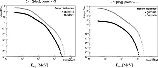
Integral energy spectrum of gamma-rays and neutrons at the Sun, emitted in the forward cone (≲10°) for 106 particles. The results are given by the Monte Carlo calculation based on GEANT4. The left-hand panel shows the integral energy spectrum of neutrons (+) and gamma-rays (•) for proton incidence, and the right-hand panel corresponds to the incidence of helium ions. Either protons or helium ions were injected into the solar atmosphere with a power-law index of 3. The maximum energy of ions is set at 100 GeV per nucleon. The fluxes represent the forward-emitted neutrons and gamma-rays to a solar atmosphere thickness of 10 g cm−2. The vertical number represents the expected number of secondary particles (n, γ) with energy higher than En,γ for the injection of 106 protons or helium ions into the solar surface.
6.2 Comparing the simulation results with actual observational results
From the value presented in the previous section, the intensity of n for the first peak is estimated as (73 ± 24) neutrons cm−2, while the flux of γ rays is (8.3 ± 1.7) × 104 photons m−2 min−1 or (0.14 ± 0.03) photons cm−2 s−1. This value may be given for the peak time during 19:57–19:58 UT, since solar neutrons are assumed to be dominantly produced during this time. The error bars stem from the variation of the estimated flux at the top of the atmosphere due to the variation of the power-law index γ between 3 and 5. The technical details of the derivation of these numbers are provided in appendix 2.
The |$n/{\rm{\gamma }}$| ratio at the energy En,γ ≥ 100 MeV is estimated as (9.5 ± 4.5), under the assumption that those solar neutrons are produced in one minute at the peak time of the gamma-ray flux. The above observational results compared with the prediction of the Monte Carlo simulation (figure 8) imply that protons were still dominantly involved in the accelerated ions in the impulsive phase of the SOL2011-03-07 flare.
7 Comparison of observed intensities between SNT and FERMI-LAT
Let us compare the flux observed using the FERMI-LAT instrument with the flux estimated based on observational results using the Sierra Negra SNT. The gamma-ray flux near the Earth measured by FERMI-LAT in association with the 2011 March 7 flare around 20:15 UT was reported by Ackermann et al. (2014) as (1.7 ± 0.2 + 0.2 − 0.1)×10−5 photons cm−2 s−1 for Eγ > 100 MeV. In contrast, the gamma-ray flux of Eγ > 100 MeV estimated from the counting rate by the N1 channel of the SNT is (1.4 ± 0.3) × 10−1 photons cm−2 s−1. The result of the SNT is around four orders of magnitude higher than the value reported from FERMI-LAT. However, the result may not be surprising. The SNT value corresponds to the impulsive phase, while the FERMI-LAT value was registered in the later phase of the flare, even if only 15 min later, considering that the impulsive phase may be very brief. Many previous observations indicate a similar trend. For example, the emission time profile of the 2.223 MeV nuclear line gamma-rays showed similar trends (for example, figure 4 of Rank et al. 2001). In the flare of 1991 June 11, Kanbach et al. (1993) and Rank et al. (2001) reported that the intensity of gamma-rays at the impulsive phase was ∼1000 times more intense than in the gradual phase.
The data taken during flare impulsive phases by FERMI-LAT are not so many. As examples, we may present the fluxes of high-energy gamma-rays observed by FERMI-LAT in the impulsive phase. They were reported as ∼6.5 × 10⁻³ photons cm−2 s−1 and ∼3.2 × 10⁻² photons cm−2 s−1 for the two flares on SOL2010-06-12 (M2.0) and SOL2017-09-10 (X8.2), respectively. The present gamma-ray flux derived from the SNT measurements (∼1.4 × 10⁻¹ photons cm−2 s−1) is 20 times higher than that determined for the event SOL2010-06-12; that flare was a very short impulsive flare M2.0 that lasted only 20 s, while the flare of SOL2011-03-07 was M3.7 and continued for more than 20 min (from start time to peak time). Therefore, it would be natural that the intensity of gamma-rays in the impulsive phase of SOL2011-03-07 is stronger than that of SOL2010-06-12. On the other hand, in comparison with the flare of SOL2017-09-10, the flux of the SOL2011-03-07 event is about four times more intense, since the flare of SOL2017-09-104 was a limb flare, part of the secondary gamma-rays might attenuate when they escape from the solar atmosphere. The details will be discussed elsewhere (Kamiya et al. 2019).
We depict the following scenario on the second enhancement recorded by the SNT at ∼20:36 UT. The second peak may have already started at ∼20:10 UT, independent of the first flare. The situation may be similar to the time development of SOL2017-09-10. In that flare, according to an early analysis,4 a weak emission of gamma-rays with energies higher than 80 MeV was first observed. The weak emission was almost proportional to the time profile of the intensity of hard X-rays. At that time, the intensity of gamma-rays (E > 80 MeV) was estimated as 6 × 10⁻⁴ photons cm−2 s−1. However, after 2 min, high-energy gamma-rays were dominantly emitted and the emission continued for more than 8 min. The intensity reached ∼4 × 10⁻² photons cm−2 s−1, almost two orders of magnitude higher than the precursor. Therefore, in the SOL2011-03-07 case, a weak emission of gamma-rays (∼2 × 10⁻⁵ photons cm−2 s−1 from ∼20:10 to 20:37 UT was followed by a strong emission of high-energy gamma-rays from 20:37 to 21:03 UT. The first flare may have produced seed particles needed for the acceleration of high-energy particles in the second peak. The intensity of the presumed gamma-rays observed by the ground-based detector presented here might be the highest intensity of solar gamma-rays reported until now. Even for this extreme situation, the scenario described here is a consistent, plausible physical environment.
8 Summary and conclusion
We have reevaluated the time profiles of high-energy photons and neutrons observed with several detectors in association with the M3.7 flare on 2011 March 7. The different intensities recorded by SN-SNT and SEDA may be consistently explained to be due to solar gamma-rays, when data are compared with a new Monte Carlo calculation based on the GEANT4 program.
To the best of our knowledge, there is no previous report on the detection of solar gamma-rays with a ground-based detector. Therefore, this may be the first observation of solar gamma-rays at the Earth's surface. Many cosmic ray detectors are located in high mountains. Thus, it is of paramount importance to search for solar gamma-ray signals with these instruments as they are a useful tool to study particle acceleration processes during high-energy events in the solar atmosphere.
Footnotes
GOES data 2011, SWPC PRF 1854 〈ftp://ftp.swpc.noaa.gov/pub/warehouse/2011〉.
RHESSI web site 〈http://sprg.ssl.berkeley.edu/∼tohban/browser/?show=grth+qlpcr〉.
SOHO LASCO CME Catalog 〈https://cdaw.gsfc.nasa.gov/CME_list/index.tml〉.
Share, G. H., & Murphy, R., 2018, presentation at Solar Energetic Particles (SEP), Solar Modulation and Space Radiation: New Opportunities in the AMS-02 Era #3, Washington D.C., 2018 April 23 to 26. 〈https://indico.cern.ch/event/685217/sessions/271288/attachments/1640707/2620375/Share_Gerald.pdf〉.
Acknowledgments
The authors wish to acknowledge the staff of the International Cosmic Ray Observatory in Tibet (organized by Academia Sinica) for keeping the detector in good condition. We thank the INAOE personnel and authorities for their continued support in providing the services needed to keep the Sierra Negra SNT functioning well. We also acknowledge UNAM-PAPIIT partial support through grant IN-104115, and particularly acknowledge the Kibo personnel at the Tsukuba Space Center (TKSC) for collecting the SEDA-NEM-FIB data every day. We specifically wish to thank Dr. T. Sakai (Nihon University), Dr. T. Yuda (ICRR, deceased), and Dr. T. Goka (JAXA) for their great contributions at the initial stage of setting up the detectors of the SNT at Mt. Sierra Negra, in the Yangbajing laboratory, and the SEDA sensor on board the ISS, respectively. We also want to thank K. Namikawa of the National Astronomical Observatory of Japan (NAOJ) in Hawaii for having kept the neutron telescope in good condition over 21 years. This work was made possible under Grant-in-Aid of Scientific Research for Priority Area 10117209 and a Grant-in-Aid of Scientific Research for Scientific Research (C) 16K05377 from the Japan Society for the Promotion of Science. Finally, the authors acknowledge the anonymous referees who have read our paper very carefully and provided many useful comments.
Potential conflicts of interest
The authors declare that they have no conflicts of interest.
Appendix 1. Another event in association with SOL2011-09-25
The detection of solar gamma-rays with a ground-based detector on 2011 March 7 is not the only event we have registered. We have found another event in association with the M7.4 medium-size flare of SOL2011-09-25. The enhancements were detected by the L1–L3 (ΔLi, i = 1–3) channels as shown in figure 9. The dashed line shows the start time of the FERMI-GBM. The excess was found in the SNT located at Yangbajing in Tibet (4300 m). The detection principle of the SNT in Tibet is the same as the SNT at Mt. Sierra Negra (Muraki 2007; Watanabe 2005). At the same time, a muon-neutron detector was operating at the same site; however, no enhancement was recorded by this detector (Zhang et al. 2005). Therefore, a possible interpretation of this excess may be due to gamma-rays in association with the M7.4 flare. The brown curve in figure 5 also supports the above interpretation of this event. The physics involved in this event will be published elsewhere.
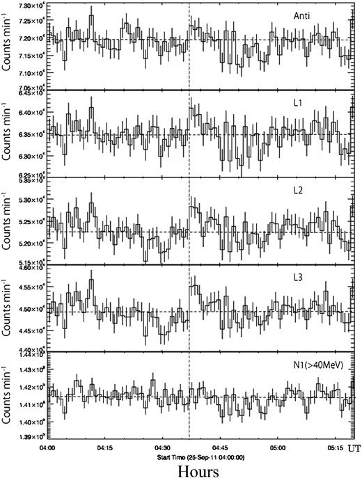
Counting rates of each channel of the SNT located at Yangbajing in Tibet (4300 m above sea level). From top to bottom: one-minute counting rates of the Anti_all, L1, L2, L3, and N1 channels are presented. The details of each channel are provided in the text. The vertical dotted line corresponds to the start time of the excess of FERMI-GBM soft gamma-rays at 04:37 UT (RHESSI website). The horizontal dashed line represents the average value of the counting rate of each channel from 04:00 to 05:20 UT. The atmospheric thickness in the solar direction was 730 g cm−2. The pressure effect has already been corrected.
Appendix 2. The attenuation of gamma-rays in the atmosphere
First of all, the threshold energy of SN-SNT is set at Eγ > 30 MeV. Therefore, in our simulation we followed gamma-rays in the atmosphere down to 30 MeV. The attenuation was evaluated as follows: We first estimated the attenuation of gamma-rays for a fixed threshold energy. Calculations were done for the different atmospheric levels of 670 g and 760 g for different times, as the solar altitude declines with time. Figure 10 shows the attenuation curves. The attenuation is evaluated for the injection of a fixed primary energy of gamma-rays into the atmosphere. Figure 10 indicates that the attenuation rate may be approximated by a straight line on a log–log plot. Therefore, the curves fit the equation Arr(E) = αE−β. Arr(E) presents the probability of arrival for an incident fixed gamma-ray energy E. The parameters α and β are given in table 4.
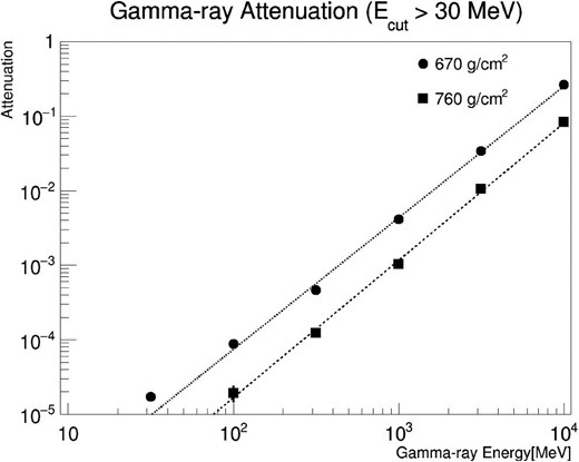
Attenuation of gamma-rays in the atmosphere as a function of the threshold energy. The upper line (•) shows the attenuation at an atmospheric depth of 670 g cm−2, while the lower line (▪) corresponds to the attenuation at an atmospheric depth of 760 g cm−2. The threshold energy is set at Eγ > 30 MeV.
Gamma-ray attenuation at corresponding atmospheric depths.
| 1 | Attenuation parameters | 670 g | 760 g |
| 2 | Photons higher than | E γ > 30 MeV | E γ > 30 MeV |
| 3 | α | 10−7.46 | 10−9.0 |
| 4 | β | 1.73 | 2.0 |
| 5 | γ = 3.0 | 31 | 6.3 |
| 6 | γ = 4.0 | 360 | 33 |
| 7 | γ = 4.5 | 1500 | 128 |
| 8 | γ = 5.0 | 6700 | 556 |
| 9 | Normalization at the flux of | 1 photon at 1 GeV | 1 photon at 1 GeV |
| 10 | Photons higher than | E γ > 100 MeV | E γ > 100 MeV |
| 11 | γ = 3.0 | 0.55 | 0.41 |
| 12 | γ = 4.0 | 0.21 | 0.27 |
| 13 | γ = 4.5 | 0.12 | 0.16 |
| 14 | γ = 5.0 | 0.064 | 0.089 |
| 15 | Normalization at the flux of | 1 photon at 30 MeV | 1 photon at 30 MeV |
With this attenuation rate, we multiply the incident power flux (E−γ) of gamma-rays by Arr(E) and integrate the product from 30 MeV to 10 GeV: ∫Arr(E) × E−γdE. Then we get the real probability of the arrival of gamma-rays with energy higher than 30 MeV: the expected number of gamma-rays at the mountain site. We tried power indexes from γ = 3 to 5, since the FERMI-LAT team estimated the initial power-law index of ions as 4.5 ± 0.5 (Ackermann et al. 2014). The numbers on rows 5–8 of table 4 indicate the number of photons just above the detector for various spectral indexes between γ = 3 and 5, when one photon with the energy of 1 GeV arrives at the top of the atmosphere. Alternatively, the values on rows 7 to 10 of table 3 represent the flux of gamma-rays with 1 GeV energy at the top of the atmosphere predicted by the present observed values like 206 or 333 counts m−2 min−1. On rows 11–14 of table 4 we present the expected rate of gamma-rays with Eγ > 100 MeV implied by the flux E > 30 MeV (the observation value). Using these numbers, we derived the possible flux at the top of the atmosphere with energies higher than Eγ > 100 MeV and compared the two fluxes observed by FERMI-LAT and SN-SNT.
For example, in the first peak we observed 43 events with Eγ > 30 MeV. We must correct the detection efficiency of gamma-rays of the detector (0.21; row 3 of table 3). Then, on the top of the detector, about 206 photons arrived. Among them, in case of the spectral index γ = 4.5, 24.7 events (= 206 × 0.12) were induced by the photons with incident energy higher than Eγ > 100 MeV. (The number 0.12 is shown on row 13 of table 4.) From figure 11 the attenuation of photons higher than 100 MeV is estimated to be 2.5 × 10⁻⁴. So we corrected the integral attenuation factor 4000 (as shown in figure 11 in appendix 3) to the number of 24.7 and obtained a possible flux of ∼98400 counts m−2 min−1. We convert this number to units of cm−2 s−1, dividing by 600000, and we got the final number of 0.16 photons cm−2 s−1 for the first peak. The intensity is four times higher than the value reported by using FERMI-LAT data for the flare of SOL2017-09-10.4
![Attenuation of primary gamma-rays in the atmosphere; (a) for the case of a power-law spectrum with an index of γ = 4.5, and (b) an exponential spectrum. The integral curve (black line) of the power-law spectrum, the absolute value is normalized at the value of the green line at the threshold energy of the detector, 30 MeV. Furthermore, the primary flux of gamma-rays is set to 1.0 at Eγ = 100 MeV [for panel (a)]. The green curve presents the integral of the product of the attenuation value for a fixed energy (purple) and the primary flux of gamma-rays (red). The attenuation factor Arr(E) is estimated by the GEANT4 code at the atmospheric depth of 760 g cm−2. (Color online)](https://oup.silverchair-cdn.com/oup/backfile/Content_public/Journal/pasj/72/2/10.1093_pasj_psz141/2/m_pasj_72_2_18_f3.jpeg?Expires=1749459440&Signature=0fSKDQNBGKGmpTHxzJ8jBTA1HsA2-vvk8GyG65wpyei1dEZD~gkOX8dQqnBuAI2Z2N7MDbKK8mMdcRtVZqnkg7nASlImHQbA81WUgaLaz23h7kqylWhpCy6NpKYnKfpbDaFXp50vVQXHmnW9H2gcpy2z32tNfQlI4~o6r3Ku86vsXOLgPm6OHbA7qq0crwztIzuM~ox~ZyClaP4yfNIQ~VV6sHvBmKH5b1-44lMN-H~fgzNMCEEE3hSpLtP7mCkCNOn3C30JL-kVRqFbZop0eO4ne4djhyNMIx0x4Dt~yWXSOx-3IQk9zNoyBuM1oexaMwxrY1tI7WiCkgpunpGuxA__&Key-Pair-Id=APKAIE5G5CRDK6RD3PGA)
Attenuation of primary gamma-rays in the atmosphere; (a) for the case of a power-law spectrum with an index of γ = 4.5, and (b) an exponential spectrum. The integral curve (black line) of the power-law spectrum, the absolute value is normalized at the value of the green line at the threshold energy of the detector, 30 MeV. Furthermore, the primary flux of gamma-rays is set to 1.0 at Eγ = 100 MeV [for panel (a)]. The green curve presents the integral of the product of the attenuation value for a fixed energy (purple) and the primary flux of gamma-rays (red). The attenuation factor Arr(E) is estimated by the GEANT4 code at the atmospheric depth of 760 g cm−2. (Color online)
Appendix 3. An integral attenuation factor
In this section we explain details on how to derive the flux at the top of the atmosphere from the data observed with a ground-based detector. For such a purpose we present two graphs: figures 11a and 11b. Figure 11a corresponds to the spectrum expected from the primary gamma-rays with the power-law index of γ: E−γ. On the other hand, figure 11b corresponds to the spectrum of gamma-rays with the exponential shape e(-E/130 MeV). The purple line is that predicted by the Monte Carlo simulation for the attenuation of gamma-rays in the atmosphere as a function of the incident energy. The result is well described by a straight line on the log–log plot. The parameters are given in table 4 and the explanations are in appendix 2.
The initial gamma-ray spectrum at the top of the atmosphere is presented by the red line in the cases of the power law and the exponential shape. The results of the multiplication of the two numbers, i.e., the attenuation factor Arr(E) × flux, are shown by the green curves in the figures. In case of the power-law spectrum, the green curve is well approximated by the straight line on the log–log plot. In the case of a power-law index of |${\rm{\gamma \ }} = 4.5$|, the index of the green line is 11|$/$|4 = 2.75 (E−11/4). Present instruments record the integral value of gamma-rays with energy higher than 30 MeV (not the differential value at Eγ = 30 MeV). Therefore, we must take into account the contribution from higher-energy components involved in the triggered events above 30 MeV. For this reason, we draw the integral curves in figure 11. They are presented by the black curve normalized at the value of the green curve at 30 MeV. Using this curve, we can derive the intensity at the top of the atmosphere. For example, at 100 MeV, we notice that the difference between the red and black curves is about 4000. Therefore, we estimate the attenuation factor to be 4000. In this way, we estimate the incident flux of gamma-rays produced in the impulsive phase of the SOL2011-03-07 event.
References
