


Abstract
We report on a possible cloud–cloud collision in the DR 21 region, which we found through molecular observations with the Nobeyama 45 m telescope. We mapped an area of ∼8′ × 12′ around the region with 20 molecular lines including the 12CO(J = 1–0) and 13CO(J = 1–0) emission lines, and 16 of them were significantly detected. Based on the 12CO and 13CO data, we found five distinct velocity components in the observed region, and we call the molecular gas associated with these components “−42,”“−22,” “−3,” “9,” and “17” km s−1 clouds, after their typical radial velocities. The −3 km s−1 cloud is the main filamentary cloud (|$\sim 31000\, M_{\odot }$|) associated with young massive stars such as DR21 and DR21(OH), and the 9 km s−1 cloud is a smaller cloud (|$\sim 3400\, M_{\odot }$|) which may be an extension of the W75 region in the north. The other clouds are much smaller. We found a clear anticorrelation in the distributions of the −3 and 9 km s−1 clouds, and detected faint 12CO emission which had intermediate velocities bridging the two clouds at their intersection. These facts strongly indicate that the two clouds are colliding against each other. In addition, we found that DR21 and DR21(OH) are located in the periphery of the densest part of the 9 km s−1 cloud, which is consistent with results of recent numerical simulations of cloud–cloud collisions. We therefore suggest that the −3 and 9 km s−1 clouds are colliding, and that the collision induced the massive star formation in the DR21 cloud. The interaction of the −3 and 9 km s−1 clouds was previously suggested by Dickel, Dickel, and Wilson (1978, ApJ, 223, 840), and our results strongly support their hypothesis of the interaction.
1 Introduction
DR21 is a small H ii region (∼30′ × 30′) in the Cyg X region and is very bright in the radio continuum (Wendker 1984) and in the infrared vibration line of molecular hydrogen tracing powerful outflow(s) driven by extremely luminous (|${\sim} 10^{5}\, L_\odot$|) young stellar objects (YSOs) forming there (e.g., Garden et al. 1986, 1991). DR21 hosts a cluster that has a high star density (∼1 × 10³ stars pc−2, Kuhn et al. 2015) and it presumably includes several O-type stars (Harris 1973; Roelfsema et al. 1989; Cyganowski et al. 2003) as well as very young members that can be classified as Class I or earlier (Marston et al. 2004). The natal cloud of DR21 is a dense massive filament extending over ∼15′ in the north–south direction, and other massive YSOs known as DR21(OH) (e.g., Norris et al. 1982) as well as W75S-FIR1, W75S-FIR2, and W75S-FIR3 (Harvey et al. 1986) are associated with the cloud.
A number of observations have been conducted toward this cloud. Dust continuum observations have unveiled the global structure of the cloud (e.g., Hennemann et al. 2012), and scores of YSOs and dense cloud cores have been found along the ridge of the filamentary cloud (e.g., Kumar 2006; Motte et al. 2007). Extensive molecular observations in the millimeter wavelengths have also been carried out and various molecular lines such as CO, SiO, CH3OH, and H2CS have been detected (e.g., Loren & Wootten 1986; Kalenskii & Johansson 2010; Schneider et al. 2010). Energetic molecular outflows have been revealed and studied in detail (e.g., Garden et al. 1986; Davis et al. 2007; Zapata et al. 2012; Smith et al. 2014; Duarte-Cabral et al. 2014; Ching et al. 2018). Recent parallax measurements of DR21 indicate a distance of |$1.50^{+0.08}_{-0.07}\:$|kpc (Rygl et al. 2012), which we adopt as the distance of the DR21 cloud in this paper.
It is known that there are two main velocity components toward the DR21 cloud. One is at VLSR ≃ −3 km s−1 and which comes from the main cloud forming the massive YSOs. The other is at ∼9 km s−1 and which may originate from the W75 region in the north. In an early molecular study of this region, Dickel, Dickel, and Wilson (1978) suggested that the two clouds are interacting with each other, based on the results of their 12CO and 13CO observations. Such interaction (cloud–cloud collisions) should sufficiently compress the clouds and may induce massive star formation. The process of cloud–cloud collisions have long been investigated theoretically (e.g., Scoville et al. 1986; Habe & Ohta 1992; Tan 2000; Dobbs 2015; Duarte-Cabral et al. 2011; Matsumoto et al. 2015; Wu et al. 2017a, 2017b; Takahira et al. 2018). Clear observational evidence of the actual cloud–cloud collisions was first discovered by Hasegawa et al. (1994) toward the Sgr B2 giant molecular cloud. More recently, a quantity of evidence of cloud–cloud collisions has been found in many massive star-forming regions (e.g., Higuchi et al. 2009; Torii et al. 2011; Nakamura et al. 2014; Fukui et al. 2018; Nishimura et al. 2018), suggesting that the cloud–cloud collisions could be one of the major triggers of massive star formation.
It is very possible that the massive star formation in the DR21 cloud was also triggered by such cloud–cloud collisions. The suggestion of Dickel, Dickel, and Wilson (1978) is important, but their original 12CO and 13CO data were obtained in 1970s with the NRAO 11 m telescope and are rather poor compared to those obtained by more recent instruments. In addition, their suggestion is based only on a positional coincidence of the two clouds on a large scale and a velocity gradient of the cloud at 9 km s−1. A more sensitive dataset as well as detailed analyses are definitely needed to confirm and develop their hypothesis. For this purpose, we have carried out observations toward the DR21 cloud with various molecular lines at much higher angular resolutions using the 45 m telescope at the Nobeyama Radio Observatory (NRO).
The observations presented in this paper were made as a part of “Star Formation Legacy Project” at the NRO (led by F. Nakamura) to observe star-forming regions such as Orion A, Aquila Rift, M|$\, 17$|, and a few other clouds such as the Northern Coalsack (NCS). An overview of the project (Nakamura et al. 2019a) and detailed observational results for the individual regions are given in other articles (Orion A: Nakamura et al. 2019b; Ishii et al. 2019; Tanabe et al. 2019, Aquila Rift: Shimoikura et al. 2019b; Kusune et al. 2019, M|$\, 17$|: Shimoikura et al. 2019a; Nguyen Lu’o’ng et al. 2019; Sugitani et al. 2019, NCS: Dobashi et al. 2019).
In this paper, we report results of the observations toward the DR21 cloud. We describe the observational procedures in section 2. We detected five velocity components including those at VLSR ≃ −3 and 9 km s−1, and find a clear anticorrelation in their spatial distributions. These results are shown in section 3. In section 4, we discuss the possible cloud–cloud collisions of the two velocity components, and summarize our conclusions in section 5.
2 Observations
Observations were carried out with the NRO 45 m telescope in the period between 2013 March and 2013 May as well as in 2014 April. We observed 20 molecular emission lines at 86–115 GHz including the 12CO(J = 1–0), 13CO(J = 1–0), C18O(J = 1–0), HCO+(J = 1–0), and SiO(J = 2–1, v = 0) lines. The observed lines are summarized in table 1. As the front end, we used the SIS receiver named Tz (Nakajima et al. 2013) which provided a typical noise temperature of Tsys ≃ 200 K including the atmosphere. As the back end, we used the SAM45 (Kamazaki et al. 2012) which consists of 16 independent digital spectrometers having 4096 channels covering the 125 MHz bandwidth with the 30-kHz resolution. The frequency resolution corresponds to the ∼0.1 km s−1 velocity resolution at 110 GHz.
Observed molecular lines.*
| Molecule | Transition | Rest frequency | ΔTmb | Detection | Figure |
|---|---|---|---|---|---|
| (GHz) | (K) | number | |||
| 12CO | J = 1–0 | 115.271202 | 1.4 | Y | 1a |
| CN | J = 3/2–1/2 | 113.490982 | 1.3 | Y | 11a |
| CCS | N, J = 9, 8–8, 7 | 113.410204 | 1.5 | N | ... |
| C17O | J = 1–0, F = 7/2–5/2 | 112.358988 | 1.0 | Y | 11b |
| CH3CN | 6(2)–5(2), F = 7–6 | 110.375052 | 0.6 | N | ... |
| 13CO | J = 1–0 | 110.201354 | 0.7 | Y | 1b |
| NH2D | 1(1,1)0–1(0, 1)0+ | 110.153599 | 1.0 | N | ... |
| C18O | J = 1–0 | 109.782173 | 0.6 | Y | 1c |
| H2CS | 3(1,3)–2(1,2) | 101.477885 | 0.6 | Y | 11c |
| HC3N | J = 11 − 10 | 100.076386 | 0.5 | Y | 11d |
| SO | N, J = 5, 4–4,4 | 100.029565 | 0.3 | N | ... |
| SO | N, J = 2, 3–1,2 | 99.299905 | 0.3 | Y | 11e |
| CS | J = 2 − 1 | 97.980953 | 0.3 | Y | 1d |
| CH3OH | 2(0,2)–1(0, 1)A++ | 96.741377 | 0.5 | Y | 11f |
| C34S | J = 2 − 1 | 96.412950 | 0.4 | Y | 11g |
| CH3OH | 2(1,2)–1(1, 1)A++ | 95.914310 | 0.5 | Y | 11h |
| HCO+ | J = 1–0 | 89.188526 | 0.3 | Y | 1e |
| HCN | J = 1–0, F = 2–1 | 88.6318473 | 0.2 | Y | 11i |
| SiO | J = 2–1, v = 0 | 86.846995 | 0.2 | Y | 1f |
| H13CO+ | J = 1–0 | 86.754288 | 0.2 | Y | 11j |
*The rest frequencies are taken from Splatalogue. ΔTmb is the 1σ noise level measured for a velocity resolution of 0.1 km s−1. “Y’ and ‘N” in the fifth column mean detection and non-detection, respectively. “Figure number” in the last column denotes the figure numbers where intensity distributions of the detected lines are displayed.
We employed the On-The-Fly (OTF; Sawada et al. 2008) technique to map an area of ∼5′ × 10′ or ∼8′ × 12′ depending on the molecular lines to cover most of the extent of the DR21 cloud. The OFF (i.e., emission-free) position was chosen to be RA(J2000.0) |$= {20^{\rm h}57^{\rm m}5{^{\rm s}_{.}}04}$| and Dec(J2000.0) |$= 39^{\circ }{19^{\prime }59{^{\prime \prime}_{.}}4}$|. Intensity calibration was done with the standard chopper-wheel method (Kutner & Ulich 1981), and spectra in units of |$T_{\rm a}^*$| were obtained. Further calibration to convert the data to Tmb was done by applying the beam efficiency of the 45 m telescope which changes from η = 35.9% at 86 GHz to 30.4% at 115 GHz. Pointing accuracy was better than 5′, as was checked by observing the SiO maser sources T-Cep and IRC +60334 every ∼2 hr during the observations.
Data reduction was done with a software package named NOSTAR. We removed the linear baselines from the spectral data, and resampled the data onto the 10′ grid and then smoothed them with a Gaussian kernel to produce a spectral data cube with an angular resolution of ∼23′ (FWHM) and velocity resolution of 0.1 km s−1. The noise levels of the final spectral data are in the range ΔTrms = 0.2–1.5 K in units of Tmb for the velocity resoluton of 0.1 km s−1, as summarized in table 1.
3 Results
3.1 Molecular distributions
As indicated in table 1, 16 molecular lines were detected in the observed region. Among these, we show in figure 1 the velocity-integrated intensity maps of six molecular lines which we use to investigate the structures of the DR21 cloud in this paper. We provide intensity maps of the other 10 molecular lines in the appendix (figure 11). In figure 1, we indicate locations of five well-known YSOs, i.e., DR21, DR21(OH), W75S-FIR1, W75S-FIR2, and W75S-FIR3, the coordinates of which are taken from Motte et al. (2007). Some of the emission lines, such as HCO+(J = 1–0), have already been observed by earlier studies (e.g., Dickel et al. 1978; Schneider et al. 2010), and their distributions are similar to those shown in the figure.
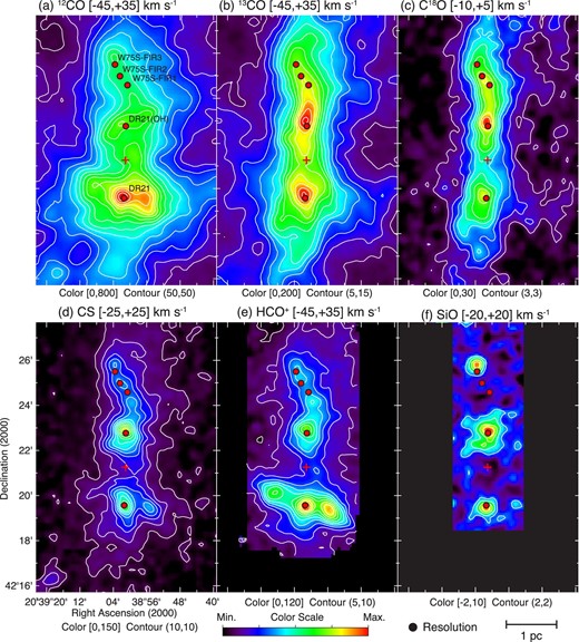
Velocity-integrated intensity maps of the observed emission lines. Molecular lines and LSR velocity ranges used for the integration are denoted above each panel. A set of the minimum and maximum values of the color scale is given in the brackets, and a set of the lowest contours and the contour intervals is given in the parentheses below each panel (in units of K km s−1). Red circles denote positions of YSOs, and plus signs denote the intensity peak position of the 9 km s−1 cloud. Areas observed in HCO+ and SiO are smaller than those observed in the other molecular lines. The filled circle below panel (f) denotes the angular resolution of the maps (23′). Molecular lines not discussed in the main text are shown in the appendix (figure 11). (Color online)
The molecular lines are strongly detected especially toward DR21 and DR21(OH). In figure 2, we show some spectra observed toward the five YSOs shown in figure 1 as well as toward a position labeled “9 km s−1 cloud” in table 2 (see subsection 3.2). In the 12CO, 13CO, and C18O spectra, some well-separated, distinct velocity components can be seen. We fitted the individual components seen in the CO lines with a Gaussian function. In table 2, we summarize the peak brightness temperature Tmb, the centroid velocity VLSR, and the FWHM line width ΔV that best fits the spectra.
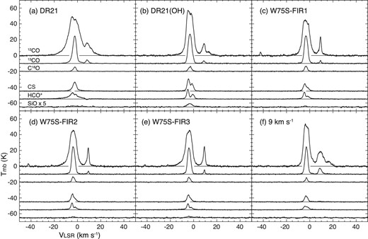
12CO, 13CO, C18O, CS, HCO+, and SiO spectra observed toward the five YSOs as well as toward the intensity-peak position of the 9 km s−1 cloud. The 13CO, C18O, CS, HCO+, and SiO spectra are offset by −10, −20, −45, −55, and −65 K, respectively. The SiO spectra are scaled up by a factor of 5.
Gaussian parameters of the CO lines.*
| Position | RA, Dec (J2000.0) | |$T^{^{12}{\rm CO}}_{\rm mb}$| | |$V^{^{12}{\rm CO}}_{\rm LSR}$| | |$\Delta V^{^{12}{\rm CO}}$| | |$T^{^{13}{\rm CO}}_{\rm mb}$| | |$V^{^{13}{\rm CO}}_{\rm LSR}$| | |$\Delta V^{^{13}{\rm CO}}$| | |$T^{{\rm C^{18}O}}_{\rm mb}$| | |$V^{{\rm C^{18}O}}_{\rm LSR}$| | |$\Delta V^{{\rm C^{18}O}}$| | |
|---|---|---|---|---|---|---|---|---|---|---|---|
| (hms) | (° ′ ′) | (K) | (km s−1) | (km s−1) | (K) | (km s−1) | (km s−1) | (K) | (km s−1) | (km s−1) | |
| DR21 | 20 39 01.4 | 42 19 34 | 48.4 | −3.0 | 11.3 | 34.1 | −2.5 | 3.8 | 5.3 | −2.4 | 3.1 |
| 12.4 | 9.7 | 6.7 | 4.1 | 8.3 | 3.2 | ... | ... | ... | |||
| DR21(OH) | 20 39 01.0 | 42 22 46 | 59.3 | −3.3 | 6.8 | 37.8 | −3.1 | 3.8 | 5.7 | −3.0 | 3.3 |
| 12.5 | 9.0 | 4.8 | 3.1 | 8.8 | 2.5 | ... | ... | ... | |||
| W75S-FIR1 | 20 39 00.6 | 42 24 35 | 46.7 | −3.2 | 7.1 | 36.0 | −3.2 | 3.5 | 6.6 | −3.2 | 2.8 |
| 21.0 | 9.2 | 2.1 | 3.4 | 9.3 | 1.6 | ... | ... | ... | |||
| W75S-FIR2 | 20 39 02.4 | 42 24 59 | 46.2 | −3.8 | 7.0 | 35.2 | −3.6 | 3.4 | 6.6 | −3.6 | 2.7 |
| 21.0 | 9.2 | 2.2 | 3.4 | 9.3 | 1.6 | ... | ... | ... | |||
| W75S-FIR3 | 20 39 03.6 | 42 25 30 | 46.1 | −4.1 | 6.6 | 33.7 | −3.9 | 3.2 | 5.9 | −3.9 | 2.7 |
| 22.7 | 9.2 | 2.2 | 5.3 | 9.3 | 1.3 | ... | ... | ... | |||
| 9 km s−1 | 20 39 01.0 | 42 21 17 | 55.1 | −2.8 | 5.7 | 34.5 | −2.9 | 2.9 | 5.1 | −2.8 | 2.3 |
| cloud | 18.2 | 9.2 | 6.7 | 7.3 | 8.9 | 3.2 | ... | ... | ... | ||
| 5.1 | 16.9 | 4.4 | ... | ... | ... | ... | ... | ... | |||
*The table lists the Gaussian parameters of the velocity components seen in the 12CO, 13CO, and C18O spectra in figure 2. Coordinates of the YSOs are taken from Motte et al. (2007): DR21, DR21(OH), W75S-FIR1, W75S-FIR2, and W75S-FIR3 correspond to N|$\, 46$|, N|$\, 44$|, N|$\, 43$|, N|$\, 51$|, and N|$\, 54$| in their table 1, respectively. The peak brightness temperature Tmb, the centroid velocity VLSR, and the line width ΔV (FWHM) are measured by fitting the observed spectra with a Gaussian function with 1–3 components.
Five velocity components can be recognized in the CO lines. The brightest component in CO is found at VLSR ≃ −3 km s−1 which originates from the main body of the DR21 cloud, and the second brightest component is seen at VLSR ≃ 9 km s−1 which may be a part of the W75 region. These velocity components are consistent with those found by earlier studies (e.g., Dickel et al. 1978; Schneider et al. 2010). In our data, another velocity component is seen at VLSR ≃ 17 km s−1 in the 12CO spectrum shown in figure 2f. Furthermore, weak emission is seen at VLSR ≃ −42 km s−1 in 12CO only around W75S-FIR1 and W75S-FIR2 (figures 2c and 2d). In addition, there is faint 12CO emission (≲5 K) around −22 km s−1 in the northwestern corner of the mapped area (figure 3b). In this paper, we will refer to molecular clouds associated with these velocity components as “−42,” “−22,” “−3,” “9,” and “17” km s−1 clouds, after their typical radial velocities and following the nomenclature of Dickel, Dickel, and Wilson (1978).
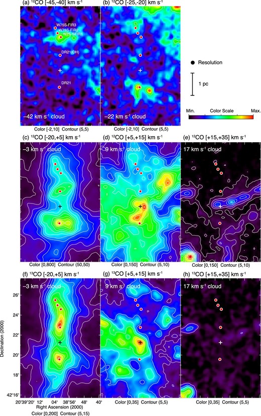
Distributions of the −42, −22, −3, 9, and 17 km s−1 clouds. Panels (a)–(e) are the channel maps of the 12CO emission line, and panels (f)–(h) are those of the 13CO emission line which are made for the same velocity intervals as for panels (c)–(e) in this order. Velocity intervals used for the integration are denoted above each panel. Others are the same as in figure 1. (Color online)
3.2 Anticorrelations and masses of the clouds
In this paper, we will mainly use the 12CO and 13CO data to investigate the distribution of the clouds as well as their possible interaction. Figure 3 shows the channel maps of the 12CO and 13CO emission lines integrated over different velocity ranges indicated on the top of each panel. In the figure, panel (a) shows the 12CO distribution of the −42 km s−1 cloud. The 12CO emission in the northwestern corner of panel (b) traces the −22 km s−1 cloud, but the emission in the middle of the panel entirely traces a part of the blueshifted high-velocity gas from the outflows driven by YSOs such as DR21 (see the 12CO spectra in figure 2). Panels (c)–(e) and (f)–(h) show the distributions of the 12CO and 13CO emission of the −3, 9, and 17 km s−1 clouds, respectively.
The overall distributions of the −3 and 9 km s−1 clouds on the plane of the sky is basically consistent with those found by Dickel, Dickel, and Wilson (1978), but it is noteworthy that our maps in figure 3 clearly reveal their anticorrelation: The 13CO intensity peak position of the 9 km s−1 cloud (figure 3g) coincides with the valley of the −3 km s−1 cloud (figure 3f) located in the middle of DR21 and DR21(OH). The same trend is seen in the 12CO distributions (figures 3c and 3d). This feature can be more clearly recognized in figure 4 where the 13CO and 12CO distributions of the two clouds are superposed. We further point out that in the northern part of the main filament between DR21(OH) and W75S-FIR3, there is another anticorrelation between the −3 and 9 km s−1 clouds in the 12CO intensity distributions (figure 4a).
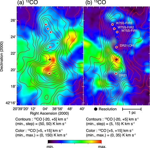
(a) 12CO and (b) 13CO distributions of the −3 km s−1 cloud (contours) and the 9 km s−1 cloud (color) which are the same as those in panels (c), (d), (f), and (g) of figure 3. Plus signs denote the intensity peak position of the 9 km s−1 cloud in 13CO. (Color online)
Such anticorrelations can be regarded as an evidence of cloud–cloud collisions which often trigger massive star formation as seen in other star-forming regions (e.g., Dobashi et al. 2014, 2019; Matsumoto et al. 2015). We will further discuss this possibility in section 4.
As a result, we found that the −3, 9, and 17 km s−1 clouds have a molecular masses of ∼31000, ∼3400, and |$\sim 500\, M_{\odot }$| within the mapped area, respectively. The −3 km s−1 cloud is the most massive among the three clouds, occupying ∼90% of the total system, and it has a much higher excitation temperature and column density [Tex ≃ 70 K and N(H2) ≃ 4.7 × 1023 cm−2 at the maximum] than the other clouds. We didn’t derive the masses of the −42 and −22 km s−1 clouds, because they are not detected in 13CO. These results are summarized in table 3.
Properties of the clouds.*
| Cloud | |$T_{\rm ex}^{\rm max}$| | N max(H2) | |$\overline{N}$|(H2) | S | M |
|---|---|---|---|---|---|
| (K) | (cm−2) | (cm−2) | (pc2) | (M⊙) | |
| −3 km s−1 | 69.5 | 4.72 × 10²³ | 2.99 × 10²³ | 1.29 | 31080 |
| 9 km s−1 | 32.3 | 2.90 × 10²² | 1.82 × 10²² | 2.56 | 3370 |
| 17 km s−1 | 37.1 | 3.41 × 10²² | 2.83 × 10²² | 0.22 | 480 |
*The table lists |$T_{\rm ex}^{\rm max}$| the maximum excitation temperature, Nmax(H2) the maximum H2 column density, |$\overline{N}$|(H2) the mean H2 column density, S the surface area defined at one half of the Nmax(H2) level, and M the total mass of the −3, 9, and 17 km s−1 clouds within the region displayed in figure 3. |$\overline{N}$|(H2) is the average value within S.
The relation of the two major clouds at −3 and 9 km s−1 is of particular interest, and we briefly estimate whether they are gravitationally bound or not. The −3 km s−1 clouds have an apparent size of ∼8′ × 2′ in 13CO with a geometrical mean radius of |$\sqrt{8^{\prime } \times 2^{\prime } }/2=2^{\prime }$|, corresponding to a radius of R = 0.9 pc at a distance of 1.5 kpc. The virial velocity calculated as |$V_{\rm vir}=\sqrt{2GM/R}$|, where M is the mass of the −3 km s−1 cloud (|$3.1\times 10^4\, M_{\odot }$|) and G is the gravitational constant, is ∼17 km s−1. This value is of the same order as the velocity separation of the −3 and 9 km s−1 clouds, 12 km s−1 in the line-of-sight velocity or |$12\sqrt{3}\simeq 21 \:$|km s−1 in 3D, and thus they could be gravitationally bound if they are located at the same distance.
3.3 Molecular outflows and the SiO emission
In some of the emission lines observed, we detected molecular outflows associated with YSOs embedded in the main cloud at −3 km s−1. Figure 5 displays the blue lobes [panels (a)–(c)] and red lobes [panels (d)–(f)] of the outflows detected in the 12CO, CS, and HCO+ emission lines. Though the red lobes detected in 12CO are highly contaminated by the other velocity components at 9 and 17 km s−1, they are traced clearly in the other two molecular lines. All of the blue lobes are well traced in the three molecular lines. The red and blue lobes associated with DR 21 and DR 21(OH) are huge and well-defined, whereas those in the vicinity of W75S-FIR1, W75S-FIR2, and W75S-FIR3 are not separated well and we cannot identify the definite driving source(s) at the resolution of the current observations.
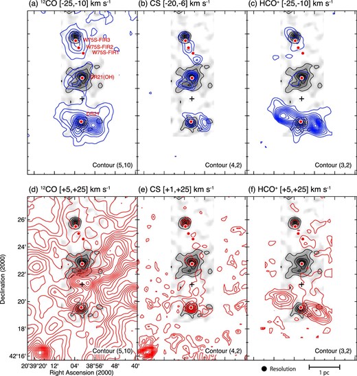
Distributions of molecular outflows detected in 12CO, CS, and HCO+ (blue and red contours) overlaid with the SiO intensity (gray-scale and black contours). Blue lobes are shown in panels (a)–(c), and red lobes are shown in panels (d)–(f). Velocity ranges used for the integration are denoted above each panel, and the lowest contours and contour intervals for the outflow lobes are indicated in the parentheses in the bottom right-hand corner of each panel. Contours for the SiO intensity are the same as in figure 1f. Red lobes in panel (d) are highly contaminated by other velocity components. (Color online)
The outflow lobes associated with DR21 appear to have rather simple structures in HCO+, extending over the length L ≃ 1 pc (measured at the lowest contours in figures 5c and 5f) from the driving source on the plane of sky. The characteristic velocity defined as the maximum velocity shift of the high-velocity gas from the systemic velocity is Vchar ≃ 25 km s−1 (measured using the blue wing of the HCO+ line in figure 6). The apparent dynamical time-scale of the outflow is therefore τage = L/Vchar ≃ 4 × 10⁴ yr, which is consistent with the results of Garden et al. (1986) if we take into account the difference of the assumed distance; they derived τage = 6–12 × 104 yr in the same way as we do, but they assumed a distance of 3 kpc. However, this time scale may be the upper limit to the actual value, because the axis of the outflow should be nearly orthogonal to the line of sight, as the red and blue lobes largely overlap on the plane of the sky. As illustrated in figure 7, if we assume that the outflow is ejected radially from DR21 at a constant speed of Voutflow and that the opening angle of the outflow is roughly θ ≃ 60°, the dynamical time-scale of the outflow can be rescaled to τage = L/Voutflow = L/Vcharsin (θ/2) ≃ 2 × 10⁴ yr.
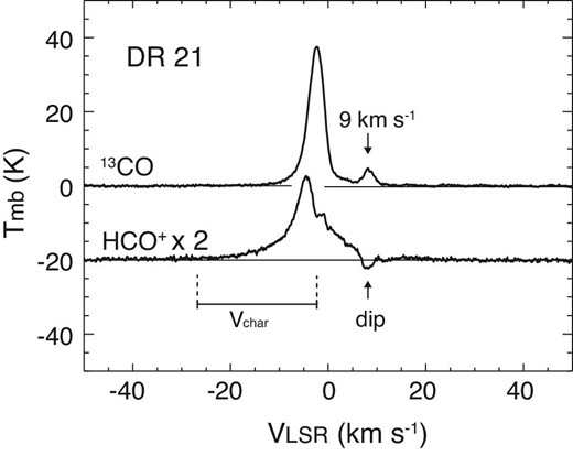
13CO and HCO+ spectra observed toward DR21, same as those shown in figure 2a. There is a dip in the HCO+ spectrum at the velocity of the 9 km s−1 cloud. The HCO+ spectrum is scaled up by a factor of 2, and is offset by −20 K. Vchar is the characteristic velocity of the outflow defined as the maximum velocity separation of the high-velocity wing(s) from the systemic velocity of DR21 (about −2.4 km s−1, see the radial velocities of 13CO and C18O in table 2).
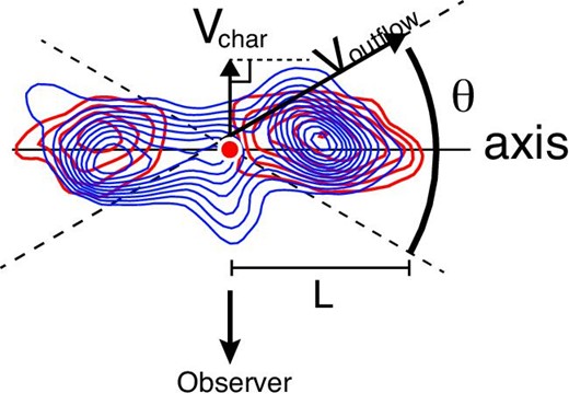
Schematic illustration of the outflow associated with DR21 plotted by the red filled circle (see subsection 3.3). (Color online)
There are apparent coincidences between the outflows and the SiO emission. The gray-scale and black contours in figure 5 represent the intensity of the SiO emission. Since Mikami et al. (1992) discovered that the SiO emission traces the shocks of the molecular outflow in LDN 1157, the emission has been recognized as a good tracer of shocks, and it has been widely used to study molecular outflows (e.g., Hirano et al. 2001; Louvet et al. 2016; Shimajiri et al. 2008, 2009). Some of the outflows in the DR21 region have been observed in SiO by earlier studies (e.g., Duarte-Cabral et al. 2014).
As seen in figures 1d and figure 5, the SiO emission is widely distributed in the observed region, but it is detected only in the three limited areas just around the YSOs, and the areas nicely overlap with the extents of the blue and/or red lobes. We therefore regard that the SiO emission detected in our observations is mostly due to the outflows.
However, we should note that the SiO emission not originating from outflows but originating from some other phenomena related to the formation of molecular clouds are recently found (e.g., Jiménez-Serra et al. 2010; Nguyen-Lu’o’ng et al. 2013). The emission is generated by low-velocity shocks such as by colliding shear or mass-accretion onto dense clumps, not by the high-velocity outflows from YSOs. Recent numerical simulations show that, when massive clouds collapse via self-gravity, striations parallel to the magnetic field naturally form (e.g., Wu et al. 2017a, 2017b) along which mass is fed from the surroundings to the central dense region. Duarte-Cabral et al. (2014) suggested that a certain fraction of the SiO emission in the DR21 region can be due to such low-velocity shocks. Global gravitational collapsing motion and convergent flows have been suggested in this region (e.g., Kirby 2009; Csengeri et al. 2011). In addition to these suggestions, we would suggest a possibility that a certain fraction of the SiO emission around DR21 and DR21(OH) might be due to shocks by the collision of the −3 and 9 km s−1 clouds, though it is very difficult to assess the contribution of this effect in the observed SiO spectra.
4 Discussion
The results shown in the previous section indicates that at least two of the clouds at −3 and 9 km s−1 are very likely to be interacting, probably colliding against each other. Such cloud–cloud collisions are known to trigger formation of massive stars and/or star clusters (e.g., Hasegawa et al. 1994; Dobashi et al. 2014; Matsumoto et al. 2015), and we suggest that formation of the massive YSOs in the DR21 region was triggered by the collision of the −3 and 9 km s−1 clouds. In the following, we further discuss the possibility of their collision and its relation to star formation based on the data obtained by our observations.
We first attempt to figure out the positional relation of the two clouds along the line of sight. At a glance of figure 4, we have an impression that the two clouds have collided and already passed through each other, and that the 9 km s−1 cloud is now located much farther from the observer than the 3 km s−1 cloud. However, the HCO+ spectrum observed toward DR21 exhibits a clear dip at VLSR = 7–10 km s−1, corresponding to the velocity of the 9 km s−1 cloud (figure 6). Such a dip is often seen in optically thick molecular lines like HCO+ toward hot regions such as compact H ii regions, and it is due to the absorption by colder gas in the foreground. Thus, the 9 km s−1 cloud should be located in front of the −3 km s−1 cloud. However, if the two components have already passed through each other and are well separated, we would not see such a dip. We therefore propose that the two clouds are attaching, or they are just crossing each other at present, and an amount of colder gas of the 9 km s−1 cloud still remains in front of the −3 km s−1 cloud (see figure 10).
As we estimated in subsection 3.3, the dynamical time-scale of the outflow associated with DR21 is τage ≃ 2 × 10⁴ yr. If we assume that the YSOs and their associated outflows were formed soon after the collision of the −3 and 9 km s−1 clouds, they have traveled only 0.2–0.3 pc along the line of sight, which is much smaller than the apparent width of the filamentary −3 km s−1 cloud or the apparent diameter of the round 9 km s−1 cloud (∼2′, corresponding to ∼1 pc). If this is the case, the two clouds should still be crossing each other, which supports the positional relation discussed in the above.
We further search for evidence of the cloud–cloud collision. If the −3 and 9 km s−1 clouds are colliding, we would expect that the gas at the intermediate velocities should exist (e.g., see figures 3 and 5 of Habe & Ohta 1992), which could be detected in the observed molecular lines. Figure 8 shows the position–velocity diagrams taken along the cuts parallel to the right ascension and declination axes crossing the peak position of the 9 km s−1 cloud. As seen in the figure, faint 12CO emission is detected along both of the cuts, bridging the −3 and 9 km s−1 clouds. We suggest that the 12CO emission with the intermediate velocities represents the gas drawn from the −3 and/or 9 km s−1 clouds. A similar feature has also been found in other star-forming regions where cloud–cloud collisions are suggested (e.g., Dobashi et al. 2019).

Position–velocity diagrams measured in 12CO along the cut A–A’ (left-hand panel) and B–B’ (right-hand panel) denoted in the middle panel. Contours start from 5 K with a step of 10 K. The horizontal white broken lines denote the position of the intensity peak position of the 9 km s−1 cloud. In the diagrams, the 12CO spectra are smoothed to the 0.5 km s−1 velocity resolution as denoted in the right-hand panel. (Color online)
We should note that the 12CO emission with the intermediate velocities could be partially due to the outflows driven by DR21 and DR21(OH). However, the outflow lobes are not overlapping with the peak position of the −9 km s−1 cloud but are extending in other directions (figure 5), and thus the emission with the intermediate velocities just around the peak position of the −9 km s−1 cloud is unlikely due to the outflows. In addition, as shown in figure 9, distribution of the 12CO emission with intermediate velocities (in the range 1 < VLSR < 5 km s−1) delineates the round edge of the densest part of the 9 km s−1 cloud (see the white ellipse pointed by an arrow in the figure), though the emission just around DR21 is apparently due to the outflow. This indicates the physical relation of the 9 km s−1 cloud and the intermediate velocity component, providing us with an additional support to suggest that the emission represents the gas drawn from the −3 and/or 9 km s−1 clouds.
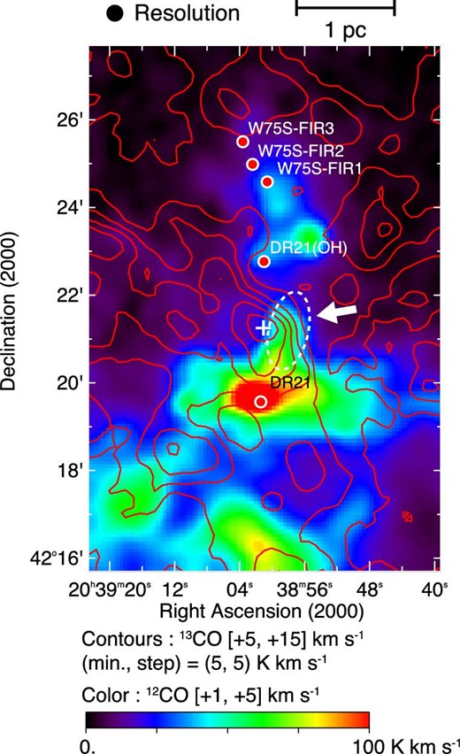
Intensity distribution of the 12CO emission line integrated over the velocity range 1 < VLSR < 5 km s−1 (color). The 13CO intensity (contours) of the 9 km s−1 cloud, same as figure 3g, is superposed for comparison. The 12CO emission in the map originates mostly from the molecular outflows, but the emission denoted by the white broken ellipse with an arrow delineates the round edge of the 9 km s−1 cloud and is likely to represent the intermediate velocity components generated by the collision. (Color online)
Hasegawa et al. (1994) discovered clear evidence of the cloud–cloud collisions in Sgr B2 for the first time; they identified a clump at VLSR = 70–80 km s−1 which fitted nicely to a hole in the cloud complex at VLSR = 40–50 km s−1, and young massive stars (including compact H ii regions and maser sources) aligned along the interface of the clump and hole. This picture appears similar to the case of the DR21 cloud: as seen in figure 4, the two massive YSOs DR21 and DR21(OH) are located in the periphery of the dense clump in the 9 km s−1 cloud. A question which immediately arises is why they are not located at the very center of the 9 km s−1 clump, which should be the center of the collision. Recent numerical simulations show that, when a time comparable to the free-fall time has passed after the collision of two clouds, a dense layer consisting of a number of clumps/cores is formed along an arc (or parabolic surface) around the axis of the collision (see figure 13 of Takahira et al. 2018). Massive stars should form there. This may be the case for DR21 and DR21(OH) as well as for the YSOs in Sgr B2.
To conclude, we suggest that the −3 and 9 km s−1 clouds are colliding against each other and that the formation of the massive YSOs, i.e., DR21, DR21(OH), W75S-FIR1, W75S-FIR2, and W75S-FIR3, were likely to be triggered by the collision. We summarize our picture of this region in a schematic illustration in figure 10. Our results strongly support the hypothesis of Dickel, Dickel, and Wilson (1978) that the two clouds are interacting with each other.
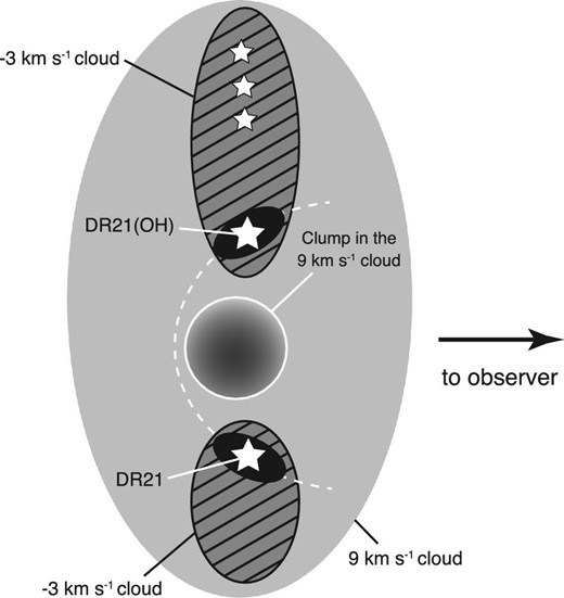
Schematic illustration of the −3 and 9 km s−1 clouds discussed in section 4. The hatched regions denote the −3 km s−1 cloud. The dense part of the 9 km s−1 cloud is shown by the gray circle with white line. The star symbols represent the YSOs, as in the other figures. Black ellipses around DR21 and DR21(OH) are the dense clumps forming along the arc (or parabolic surface) denoted by the white broken line (see text).
As summarized in table 3, the natal cloud of DR21 (the −3 km s−1 cloud) has a total mass and mean molecular column density of |$\sim 3 \times 10^4\, M_{\odot }$| and ∼3 × 1023 cm−2, respectively. It is colliding with the −9 km s−1 cloud at a relative velocity of ∼12 km s−1, and a cluster containing several O-type stars are forming in DR21 (e.g., Harris 1973). We compare these features of DR21 with other clouds producing O-type stars whose formation is supposed to be triggered by cloud–cloud collisions. Fukui et al. (2018) recently summarized properties of such clouds in the literature. Looking into their table 1, relative radial velocities of the colliding clouds are ∼10–20 km s−1, and except for a few cases, the clouds, not necessarily both of them, have a mass of ∼104–|$10^{5}\, M_{\odot }$|. Though the sample collected by Fukui et al. (2018) is rather small, parameters of the DR21 cloud are in these ranges, suggesting that DR21 may be a typical case of massive star formation induced by cloud–cloud collisions. In addition, Fukui et al. (2018) suggested that the clouds produce a so-called “super cluster” containing ∼10–20 O-type stars if the column densities of the clouds are as high as N(H2) ≃ 1023 cm−2, whereas less-dense clouds (∼1022 cm−2) produce only a single O-type star. DR21 apparently corresponds to the former case, and is similar to RCW 38 in table 1 of Fukui et al. (2018) forming a young cluster with an age of ∼0.1 Myr.
Finally, cloud–cloud collisions like that found in the DR21 cloud give us a hint to understand the onset of the formation of massive stars and star clusters. Recent studies of young clusters have shown that they are forming in massive clumps with a typical mass of |$\sim 1 \times 10^3\, M_{\odot }$| (e.g., Saito et al. 2008; Shimoikura et al. 2013). Statistical studies carried out by Shimoikura et al. (2018) have revealed that most of the clumps associated with very young clusters are gravitationally collapsing, exhibiting a clear clump-scale infalling motion with rotation (see also Shimoikura et al. 2016). Other clumps not forming clusters are expected to be in a stage prior to cluster formation and to be younger than those forming clusters. However, Shimoikura et al. (2018) found that the clumps without clusters are more evolved in terms of chemical compositions than the ones already forming clusters. They suggested that the clumps are gravitationally stable, having survived for a long time without collapsing due to cloud-supporting forces, e.g., by the magnetic field. Cloud–cloud collision should cause distortion of the magnetic field as well as sudden enhancement of gas density by compression, which should force the cloud to collapse (e.g., Wu et al. 2017a, 2017b). In the DR21 cloud, the strong magnetic field of the order of ≳1 mG is actually inferred (e.g., Lai 2003; Ching et al. 2018) and is also suggested to be interacting with the gas dynamics (Ching et al. 2018). The DR21 cloud is therefore very likely to be experiencing such a collision-induced star formation at present.
5 Conclusions
We performed molecular observations of the DR21 region using the 45 m telescope at the Nobeyama Radio Observatory (NRO). We revealed the global distributions of the molecular lines, and identified distinct clouds in this region. The main conclusions of this paper are summarized in the following points.
We mapped an area of ∼8′ × 12′ around the DR21 region with 20 molecular lines including the 12CO(J = 1–0), 13CO(J = 1–0), HCO+(J = 1–0), and SiO(J = 2 − 1, v = 0) emission lines. Among them, 16 lines were significantly detected. Based on the 12CO and 13CO data, we identified five velocity components at the radial velocities VLSR ≃ −42, −22, −3, 9, and 17 km s−1. We call the clouds associated with these components the “−42,” “−22,” “−3,” “9,” and “17” km s−1 clouds.
Based on the 12CO and 13CO data, we estimated the total molecular masses of the −3, 9, and 17 km s−1 clouds within the observed area to be ∼31000, ∼3400, and |$\sim 500\, M_{\odot }$|, respectively, assuming the local thermodynamic equilibrium (LTE). We found that there is a clear anticorrelation between the −3 and 9 km s−1 clouds, suggesting that they are colliding against each other.
The SiO(J = 2 − 1, v = 0) emission at 86.8 GHz was detected around young stellar objects in the DR21 region. Distributions of the emission line are well correlated with those of molecular outflows traced in the 12CO and a few other emission lines.
Around the intersection of the −3 and 9 km s−1 clouds, we found a velocity component that has intermediate velocities and bridges the two clouds. We also found that the geometrical relation of the YSOs and the intersection is consistent with the results of recent numerical simulations of cloud–cloud collisions. These findings indicate that the −3 and 9 km s−1 clouds are colliding, and that the collision induced the formation of the massive stars in the DR21 cloud. The interaction of the −3 and 9 km s−1 clouds in this region was first suggested by Dickel, Dickel, and Wilson (1978), and our results strongly support their hypothesis.
Acknowledgments
This work was financially supported by JSPS KAKENHI Grant Numbers JP17H02863, JP17H01118, JP26287030, and JP17K00963. The 45 m radio telescope is operated by NRO, a branch of NAOJ. YS received support from the ANR (project NIKA2SKY, grant agreement ANR-15-CE31-0017).
Appendix
Maps of the other molecular emission lines
In figure 11, we display the velocity-integrated intensity maps of the 10 molecular emission lines not shown in figure 1.
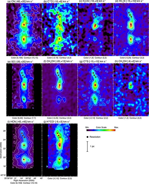
Same as figure 1, but for molecular emission lines not discussed in the main text. Areas observed in SO, HCN, and H13CO+ are smaller than those observed in the other molecular lines. For the CN, C17O, and HCN emission lines, all of the hyperfine lines are integrated. (Color online)
References
